On the Shuffling Algorithm for Domino Tilings

Abstract.

We study the dynamics of a certain discrete model of interacting particles that comes from the so called shuffling algorithm for sampling a random tiling of an Aztec diamond. It turns out that the transition probabilities have a particularly convenient determinantal form. An analogous formula in a continuous setting has recently been obtained by Jon Warren studying certain model of interlacing Brownian motions which can be used to construct Dyson’s non-intersecting Brownian motion.

We conjecture that Warren’s model can be recovered as a scaling limit of our discrete model and prove some partial results in this direction. As an application to one of these results we use it to rederive the known result that random tilings of an Aztec diamond, suitably rescaled near a turning point, converge to the GUE minor process.

1. Introduction

There has been a lot of work in recent years connecting tilings of various planar regions with random matrices. One particular model that has been intensely studied is domino tilings of a so called Aztec diamond. One way to analysing that model, [johansson:arctic_circle, johansson:discrete_orthogonal, johansson:gue_minors], is to define a particle process corresponding to the tilings so that uniform measure on all tilings induces some measure on this particle process.

In this article we will study the so called shuffling algorithm, described in [elkies:alternating_sign_matrices_II, propp:generalized_domino], which in various variants can be used either to count or to enumerate all tilings of the Aztec diamond or to sample a random such tiling.

The sampling of a random tiling by this method is an iterative process. Starting with a tiling of an order $n-1$ Aztec diamond, a certain procedure is performed, producing a random tiling of order $n$. This procedure is usually described in terms of the dominoes which should be moved and created according to a certain procedure. We will instead look at this algorithm as a certain dynamics on the particle process mentioned above.

The detailed dynamics of the particle process will be presented in section 2 and how it is obtained from the traditional formulation of the shuffling algorithm is presented in section 4. For now, consider a process $\mathpzc{X}(t)=(X^{1}(t),\dots,X^{m}(t))$ for $t=0$, $1$, $2$, …, where $X^{k}(t)=(X^{k}_{1}(t),\dots,X^{k}_{k}(t))\in\mathbb{Z}^{k}$. The quantity $X^{j}_{i}(t)$ represents the position of the $i$:th particle on line $j$ after $t-j$ steps of the shuffling algorithm have been performed. (The reason for the $t-j$ is technical convenience.) We will show that

Theorem 1.1.

For fixed $k$, consider only the component $X^{k}(t)$ from $\mathpzc{X}(t)$ rescaled according to

(1) $$\tilde{X}^{n}_{i}(t)=\frac{X^{n}_{i}(Nt)-\frac{1}{2}Nt}{\frac{1}{2}\sqrt{N}}$$

and defined by linear interpolation for non-integer values of $Nt$. The process $\tilde{X}^{n}(t)$ converges to a Dyson Brownian motion with all particles started at the origin as $N\rightarrow\infty$, in the sense of convergence of finite dimensional distributions.

The full process $(\mathpzc{X}(t))_{t=0,1,\dots}$ has remarkable similarities to, and is we believe a discretization of, a process studied recently by Warren, [warren:dyson_brownian_motions]. It consists of many interlaced Dyson Brownian motions and is here briefly described in section 3. We will denote that process $(\mathbf{X}(t))_{t\geq 0}$. There is reason to believe the following.

Conjecture.

Consider the process $(\mathpzc{X}(t))_{t=0,1,\dots}$ rescaled according to

(2) $$\tilde{X}^{n}_{i}(t)=\frac{X^{n}_{i}(Nt)-\frac{1}{2}Nt}{\frac{1}{2}\sqrt{N}}$$

and defined by linear interpolation for non-integer values of $Nt$. The process $\tilde{\mathpzc}{X}(t)$ converges to Warren’s process $\mathbf{X}(t)$ as $N\rightarrow\infty$, in the sense of convergence of finite dimensional distributions.

The key to our asymptotic analysis of the shuffling algorithm is that the transition probabilities of $(X^{k},X^{k+1})$ can be written down in a convenient determinantal form, see proposition 3.2. These formulas mirror beautifully formulas obtained by Warren.

As an application of our results we will use it to rederive an asymptotic result about random tilings near the point where the arctic circle touches the edge of the diamond. This result was first stated in [johansson:arctic_circle] and proved in [johansson:gue_minors].

Recall that the Gaussian Unitary Ensemble, or GUE for short, is a probability measure on Hermitian matrices with density $Z_{n}^{-1}e^{-\operatorname{Tr}H^{2}/2}$ where $Z_{n}$ is a normalisation constant that depends on the dimension $n$ of the matrix. Let $H=(h_{rs})_{1\leq r,s\leq n}$ a GUE matrix and denote its principal minors by $H_{j}=(h_{rs})_{1\leq r,s\leq j}$. Let $\lambda^{j}=(\lambda^{j}_{1},\dots,\lambda^{j}_{j})$ be the eigenvalues of $H_{j}$. Then $\Lambda=(\lambda^{1},\dots,\lambda^{n})\in\mathbb{R}^{n(n+1)/2}$ is the so called GUE minor process.

Theorem 1.2 (Theorem 1.5 in [johansson:gue_minors].).

Let the $\mathbb{R}^{n(n+1)/2}$-valued process $\tilde{\mathpzc}{X}(t)=(\tilde{X}^{1}(t),\dots,\tilde{X}^{n}(t))$ be a rescaled version of $\mathpzc{X}(t)$ with

(3) $$\tilde{X}^{j}_{i}(t)=\frac{X^{j}_{i}(t)-\frac{t}{2}}{\frac{1}{2}\sqrt{t}}.$$

Then $\tilde{\mathpzc}{X}(t)\rightarrow\Lambda$ as $t\rightarrow\infty$ in the sense of weak convergence of probability measures.

To put this in perspective, let us note that a similar result for lozenge tilings is known from Okounkov and Reshetikhin [okounkov:birth]. They discuss the fact that, for quite general regions, that close to a so called turning point the GUE minor process can be obtained in a limit. A turning point is, just as in our situation, where the disordered region is tangent to the domain boundary.

2. The Aztec Diamond Particle Process

We will here content ourselves with stating the rules of the particle dynamics that we will study. The reader will in section 4 find a description the traditional formulation of the shuffling algorithm and how that relates to the formulas below.

Consider the process $(\mathpzc{X}(t))=(X^{1}(t),\dots,X^{n}(t))$ for $t=0$, $1$, $2$, …, where $X^{k}(t)=(X^{k}_{1}(t),\dots,X^{k}_{k}(t))\in\mathbb{Z}^{k}$. It satisfies the initial condition

(4) $$X^{k}(0)=\bar{x}^{k}$$

where $\bar{x}^{j}_{i}=i$ for $1\leq i\leq j$. At each time $t$ the process fulfils the interlacing condition

(5) $$X^{k}_{i}(t)\leq X^{k-1}_{i}(t)<X^{k}_{i+1}(t)$$

and evolves in time according to

(6) $$X^{1}_{1}(t) =X^{1}_{1}(t-1)+\beta^{1}_{1}(t)$$

$$X^{j}_{1}(t) =X^{j}_{1}(t-1)+\beta^{j}_{1}(t)$$

$$\quad-\mathbf{1}\{X^{j}_{1}(t-1)+\beta^{j}_{1}(t)=X^{j-1}_{1}(t)+1\} j\geq 2$$ for

$$X^{j}_{j}(t) =X^{j}_{j}(t-1)+\beta^{j}_{j}(t)$$

$$\quad+\mathbf{1}\{X^{j}_{1}(t-1)+\beta^{j}_{1}(t)=X^{j-1}_{j-1}(t)\} j\geq 2$$ for

$$X^{j}_{i}(t) =X^{j}_{i}(t-1)+\beta^{j}_{i}(t)$$

$$\quad-\mathbf{1}\{X^{j}_{i}(t-1)+\beta^{j}_{i}(t)=X^{j-1}_{i}(t)+1\}$$

$$\quad+\mathbf{1}\{X^{j}_{i}(t-1)+\beta^{j}_{i}(t)=X^{j-1}_{i-1}(t)\} j\geq 3 1<i<j$$ for and .

for $t=1$, $2$, …where all the $(\beta^{j}_{i}(t))_{i,j,t}$ are i.i.d. unbiased coin tosses, satisfying $\mathbb{P}[\beta^{1}_{1}(1)=0]=\mathbb{P}[\beta^{1}_{1}(1)=1]=\frac{1}{2}$.

One way to think about this is that at each time $t$, this is a set of particles on $n$ lines. The $k$:th line has $k$ particles on it at positions $X^{k}_{1}$, …, $X^{k}_{k}$. At each time step each of these particles either stays or jumps one unit step forward independent of all others except that the particles on line $k$ can force particles on line $k+1$ to jump or to stay to enforce the the interlacing condition (5). Also note that the interlacing implies that $X^{k}_{i}<X^{k}_{i+1}$ at each time $t$, i.e. two particles cannot occupy the same space at the same time.

As mentioned we can write down transition probabilities for this process on a particularly convenient determinantal form. Define $\delta_{i}:\mathbb{Z}\rightarrow\mathbb{Z}$ such that $\delta_{i}(x)=1$ if $i=x$ and $\delta_{i}(x)=0$ otherwise. Let us first introduce some notation.

$$(\phi*\psi)(x) =\sum_{s+t=x}\phi(s)\psi(t)$$ (Convolution product)

$$\phi^{(0)} =\delta_{0}$$

$$\phi^{(n)} =\phi^{(n-1)}*\phi n=1,2,\dots$$ for

$$\Delta\phi =(\delta_{0}-\delta_{1})*\phi$$ (Backward difference)

$$\Delta^{-1}\phi(x) =\sum_{y=-\infty}^{x}\phi(y)$$

$$\bar{\Delta}\phi =(-\delta_{0}+\delta_{-1})*\phi$$ (Forward difference)

$$\bar{\Delta}^{-1}\phi(x) =\sum_{y=-\infty}^{x-1}\phi(y)$$

Let $\mathpzc{W}^{n+1,n}=\{(x,y):x_{1}\leq y_{1}<x_{2}\leq\dots\leq y_{n}<x_{n+1}\}\subset\mathbb{Z}^{n+1}\times\mathbb{Z}^{n}$. For $(x,y),(x^{\prime},y^{\prime})\in\mathpzc{W}^{n+1,n}$ and $t=0,1,\dots$, define

(7) $$\mathpzc{q}_{t}^{n}((x,y),(x^{\prime},y^{\prime}))=\det\begin{bmatrix}A_{t}(x,x^{\prime})&B_{t}(x,y^{\prime})\\ C_{t}(y,x^{\prime})&D_{t}(y,y^{\prime})\end{bmatrix}$$

where

• $A_{t}(x,x^{\prime})$ is an $(n+1)\times(n+1)$-matrix where element $(i,j)$ is $\phi^{(t)}(x_{i}^{\prime}-x_{j})$,

• $B_{t}(x,y^{\prime})$ is an $(n+1)\times(n)$-matrix where element $(i,j)$ is $\Delta^{-1}\phi^{(t)}(y_{i}^{\prime}-x_{j})-\mathbf{1}\{j\geq i\}$,

• $C_{t}(y,x^{\prime})$ is an $n\times(n+1)$-matrix where element $(i,j)$ is $\Delta\phi^{(t)}(y_{i}^{\prime}-x_{j})$ and

• $D_{t}(y,y^{\prime})$ is an $n\times n$-matrix where element $(i,j)$ is $\phi^{(t)}(y_{i}^{\prime}-y_{j})$.

Let $\mathpzc{W}^{n}=\{x:x_{1}<x_{2}<\dots<x_{n}\}\subset\mathbb{Z}^{n}$ and for $x\in\mathpzc{W}^{n}$ let

(8) $$h_{n}(x)=\prod_{i<j}(x_{j}-x_{i}).$$

Finally, after all this notation, we can state a result.

Theorem 2.1.

The transition probabilities of $(X^{k},X^{k+1})$ from the process $\mathpzc{X}$ above are

(9) $$\mathpzc{q}_{t}^{k,+}((x,y),(x^{\prime},y^{\prime})):=\frac{h_{k}(y^{\prime})}{h_{k}(y)}\mathpzc{q}_{t}^{k}((x,y),(x^{\prime},y^{\prime}))$$

that is

(10) $$\mathbb{P}[(X^{k+1}(s+t),X^{k}(s+t))=(x^{\prime},y^{\prime});(X^{k+1}(s),X^{k}(s))=(x,y)]=\mathpzc{q}_{t}^{k,+}((x,y),(x^{\prime},y^{\prime})).$$

A proof is given in section 6 and the reason I defined $\mathpzc{q}_{t}^{k}$ as opposed to defining $\mathpzc{q}_{t}^{k,+}$ directly will become obvious in the next section.

Given the exact expressions above it is a very straightforward computation to integrate out the $x$ component in expression (9). We find that the transition probabilities of $(X^{k})$ from the process $\mathpzc{X}$ above is

(11) $$\mathpzc{p}_{t}^{k,+}(y,y^{\prime}):=\frac{h_{k}(y^{\prime})}{h_{k}(y)}\mathpzc{p}_{t}^{k}(y,y^{\prime})$$

where $\mathpzc{p}_{t}^{k}(y,y^{\prime}):=D_{t}(y,y^{\prime})$ given above. We recognise this as the transition probability for random walks conditioned never to intersect, a fact that is so important we state it properly.

Corollary 2.2.

The component $X^{k}(t)$ of $\mathpzc{X}(t)$ is a discrete Dyson Brownian motion of $k$ particles started at $\bar{x}^{k}$.

This fits nicely with theorem 1.1. The component $X^{k}$ from $\mathpzc{X}$ simply $k$ simple symmetric random walks conditioned never to intersect, their limit is $k$ Brownian motions conditioned never to intersect, which is exactly what $X^{k}$ from Warren’s process $\mathbf{X}$ is.

3. Interlacing Brownian motions

We will now digress a bit and summarise Warren’s work in [warren:dyson_brownian_motions], so as to see the similarities between his continuous process and our discrete process. The reader is referred to that reference for more details of the construction. Consider an $\mathbb{R}^{n+1}\times\mathbb{R}^{n}$-valued stochastic process $(Q(t))_{t\geq 0}=(X(t),Y(t))_{t\geq 0}$ satisfying an interlacing condition

(12) $$X_{1}(t)\leq Y_{1}(t)\leq X_{2}(t)\leq\dots\leq Y_{n}(t)\leq X_{n+1}(t),$$

and equations

(13) $$Y_{i}(t) =y_{i}+\beta_{i}(t\wedge\tau),$$

(14) $$X_{i}(t) =y_{i}+\gamma_{i}(t\wedge\tau)+L_{i}^{-}(t\wedge\tau)-L_{i}^{+}(t\wedge\tau)$$

where

$(\beta_{i})_{i=1}^{n}$ and $(\gamma_{i})_{i=1}^{n+1}$ are independent Brownian motions,

$\tau=\inf\{t\geq 0:Y_{i}(t)=Y_{i+1}\text{ for some $i$}\}$,

$L^{-}_{1}\equiv L^{+}_{n+1}\equiv 0$ and

(15) $$L_{i}^{+}(t) =\int_{0}^{t}\mathbf{1}(X_{i}(s)=Y_{i}(s))\,dL_{i}^{+}(s) L_{i}^{-}(t) =\int_{0}^{t}\mathbf{1}(X_{i}(s)=Y_{i-1}(s))\,dL_{i}^{-}(s)$$

are twice the semimartingale local times at zero of $X_{i}-Y_{i}$ and $X_{i}-Y_{i-1}$ respectively.

This process can be constructed by first constructing the Brownian motions $\beta_{i}$ and $\gamma_{i}$ and then using Skorokhod’s construction to push $X_{i}$ up from $Y_{i-1}$ and down from $Y_{i}$. The process is killed when $\tau$ is reached, i.e. when two of the $Y_{i}$ meet.

Warren then goes on to show that the transition densities of this process have a determinantal form similar to what we have seen in the previous section. Let $\varphi_{t}(x)=(2\pi t)^{-1/2}e^{-x^{2}/2t}$ and $\Phi_{t}(x)=\int_{-\infty}^{x}\varphi_{t}(y)\,dy$. Let $W^{n,n+1}=\{(x,y)\in\mathbb{R}^{n}\times\mathbb{R}^{n+1}:x_{1}<y_{1}<x_{2}<\dots<y_{n}<x_{n+1}\}$.

Define $q_{t}^{n}((x,y),(x^{\prime},y^{\prime}))$ for $(x,y)$, $(x^{\prime},y^{\prime})\in W^{n,n+1}$ and $t>0$ to be the determinant of the matrix

(16) $$\begin{bmatrix}A_{t}(x,x^{\prime})&B{t}(x,y^{\prime})\\ C_{t}(y,x^{\prime})&D{t}(y,y^{\prime})\end{bmatrix}$$

where

$A_{t}(x,x^{\prime})$ is an $(n+1)\times(n+1)$-matrix where element $(i,j)$ is $\varphi_{t}(x_{i}^{\prime}-x_{j})$,

$B_{t}(x,y^{\prime})$ is an $(n+1)\times(n)$-matrix where element $(i,j)$ is $\Phi_{t}(y_{i}^{\prime}-x_{j})-\mathbf{1}(j\geq i)$,

$C_{t}(y,x^{\prime})$ is an $n\times(n+1)$-matrix where element $(i,j)$ is $\varphi_{t}^{\prime}(y_{i}^{\prime}-x_{j})$ and

$D_{t}(y,y^{\prime})$ is an $n\times n$-matrix where element $(i,j)$ is $\varphi_{t}(y_{i}^{\prime}-y_{j})$.

Proposition 3.1 (Prop 2 in [warren:dyson_brownian_motions]).

The process $(X,Y)$ killed at time $\tau$ has transition densities $q^{n}_{t}$, that is

(17) $$q_{t}^{n}((x,y),(x,y))\,dx^{\prime}dy^{\prime}=\mathbb{P}^{x,y}[X_{t}\in dx^{\prime},Y_{t}\in dx^{\prime};t<\tau]$$

Warren goes on to condition the $Y_{i}$ not to intersect via so called the Doob $h$-transform. The transition densities for the transformed process are given in terms of the those for the killed process by

(18) $$q^{n,+}_{t}((x,y),(x^{\prime},y^{\prime}))=\frac{h_{n}(y^{\prime})}{h_{n}(y)}q^{n}_{t}((x,y),(x^{\prime},y^{\prime})).$$

He also shows that you can start all the $X_{i}$ and $Y_{i}$ of the transformed process at the origin by giving a so called entrance law,

(19) $$\nu_{t}^{n}(x,y):=\frac{n!}{Z_{n+1}}t^{-(n+1)^{2}/2}\exp\left\{-\sum_{i}x_{i}^{2}/(2t)\right\}\left\{\prod_{i<j}(x_{j}-x_{i})\right\}\left\{\prod_{i<j}(y_{j}-y_{i})\right\},$$

that is, showing (lemma 4 of [warren:dyson_brownian_motions]) that this expression satisfies

(20) $$\nu_{t+s}^{n}(x^{\prime},y^{\prime})=\int_{W^{n,n+1}}\nu_{s}^{n}(x,y)q_{t}^{n,+}((x,y),(x^{\prime},y^{\prime}))\,dxdy.$$

It is possible to integrate out the $X$ components in that transition density and entrance law. The result is transition density

(21) $$p^{n,+}_{t}(y,y^{\prime}):=\frac{h(y^{\prime})}{h(y)}\det D_{t}(y,y^{\prime})$$

and entrance law

(22) $$\mu^{n}_{t}(y):=\frac{1}{Z_{n}}t^{-n^{2}/2}\exp\left\{-\sum_{i}y_{i}^{2}/(2t)\right\}\left\{\prod_{i<j}(y_{j}-y_{i})\right\}^{2}.$$

Now comes the interesting part. Let $\mathbf{K}$ be the cone of points $x=(x^{1},\dots,x^{n})$ where $x^{k}=(x^{k}_{1},\dots,x^{k}_{k})\in\mathbb{R}^{k}$. Warren defines a process $\mathbf{X}(t)$ taking values in $\mathbf{K}$ such that

(23) $$X^{k}_{i}(t)=x^{k}_{i}+\gamma^{k}_{i}(t)+L_{i}^{k,-}(t)-L_{i}^{k,+}(t)$$

where the $(\gamma_{i}^{k})_{i,k}$ are independent Brownian motions and $L_{i}^{k,+}$ and $L_{i}^{k,+}$ are continuous, increasing processes growing only when $X^{k}_{i}(t)=X^{k-1}_{i}(t)$ and $X^{k}_{i}(t)=X^{k}_{i-1}(t)$ respectively and the special cases $L^{k,+}_{k}$ and $L^{k,-}_{1}$ are identically zero for all $k$.

Think of this as essentially $n(n+1)/2$ particles performing independent Brownian motions except that the $k$ particles in $X^{k}$ can push the particles in $X^{k+1}$ up or down to enforce the interlacing condition that the whole process should stay in $\mathbf{K}$.

This full process process can be constructed inductively as follows.

1. The process $(X^{k})$ has transition densities $p^{k,+}_{t}$ and entrance law $\mu^{k}_{t}$.

2. The process $(X^{k},X^{k+1})$ has transition densities $q^{k,+}_{t}$ and entrance law $\nu^{k}_{t}$.

3. For $k=2,\dots,n-1$ the process $(X^{k+1})$ is conditionally independent of $(X^{1},\dots,X^{k-1})$ given $(X^{k})$.

4. This implies (by some explicit calculations) that $(X^{k+1})$ has transition densities $p^{k+1,+}_{t}$ and entrance law $\mu^{k+1}_{t}$.

This argument shows that the following.

Proposition 3.2 (Warren).

There exists such a process $\mathbf{X}(t)$ started at the origin and it satisfies that for $k=1$, …, $n-1$, the process $(X^{k},X^{k+1})$ has entrance law $\nu_{t}^{n}$ and transition probabilities $q^{k,+}$.

It is this process $\mathbf{X}$ that is the continuous analog of our discrete process $\mathpzc{X}$.

4. Shuffling algorithm

We will now show how relate some well known facts about sampling random tilings of an Aztec diamond before showing how to get the particle dynamics in section 2.

The Aztec diamond of order $n$, denoted $A_{n}$, is an area in the plane that is the union of those lattice squares $[a,a+1]\times[b,b+1]\subset\mathbb{R}$ that are entirely contained in $\{|x|+|y|\leq n+1\}$. $A_{n}$ can be tiled in $2^{n(n+1)/2}$ ways by dominoes of size $2\times 1$. We will be interested picking a random tiling. By random tiling in this article we will always mean that all possible tilings given the same probability.

A key ingredient of almost all results concerning tilings of this shape is the realization that one can distinguish four kinds of dominoes present in a typical tiling. The obvious distinction to the casual observer is the difference between horizontal and vertical dominoes. These can be subdivided further. Colour the underlying lattice squares black and white according to a checkerboard fashion in such a way that the left square on the top line is black. Let a horizontal domino be of type N or north if its leftmost square is black, and of type S or south otherwise. Likewise let a vertical domino be of type W or west if its topmost square is black and type E or east otherwise. In figures 1 and 2 the S and E type dominoes have been shaded for convenience.

One way of sampling from this measure is the so called shuffling algorithm, first described in [elkies:alternating_sign_matrices_II], and very nicely explained and generalised in [propp:generalized_domino]. It is an iterative procedure that given a random tiling of $A_{n}$ and some number of coin-tosses, produces a random tiling of a diamond of $A_{n+1}$. You start with the empty tiling on $A_{0}$ and you repeat this process until you have a tiling of the desired size. It is a theorem that this procedure gives all tilings equal probability, provided that the coin-tosses we have made along the way are fair.

The algorithm works in three stages. Start with a tiling $A_{n}$.

Destruction:

All $2\times 2$ blocks consisting of an S-domino directly above an N-domino are removed. Likewise all $2\times 2$ blocks of consisting of an E-domino directly to left of a W-domino are removed.

Shuffling:

All N, S, E and W-dominoes respectively move one unit length up, down, right and left respectively.

Creation:

The result is a tiling of a subset of $A_{n+1}$. The empty parts can be covered in a unique way by 2$\times$2 squares. Toss a coin to fill these with two horizontal or two vertical dominoes with equal probability.

Figure 1 illustrates the process. In the leftmost column there are tilings of successively larger diamonds. From column one to column two, the destruction step is carried out. From there to the third column, shuffling is performed. These figures contain several dots which will concern us later in this exposition. The creation step of the algorithm applied to a diamond in the last column gives (with positive probability) the diamond in the first column on the next row.

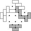
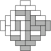
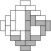
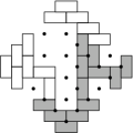
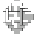
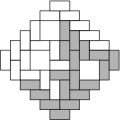
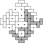
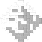
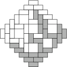
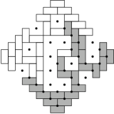
Figure 1. The shuffling procedure. S- and E-type dominoes are shaded.

To study more detailed properties of random tilings it is useful to introduce a coordinate system suited to the setting and a particle process such that the possible tilings correspond to particle configurations.

In the left picture in figure 2, the S and E type dominoes are shaded and a coordinate system is imposed on the tiling. For each tile there is exactly one of the $x$ lines and exactly one of the $y$ lines that passes through its interior. Indeed we can uniquely specify the location of a tile by giving its coordinates $(x,y)$ and type (N, S, E or W). You can see that along the line $y=k$ there are exactly $k$ shaded tiles, for $y=1\ldots 8$ where $8$ is the order of the diamond. The obvious generalisation of that statement is true for tilings of $A_{n}$ for any $n$. We shall call the occurrence of a shaded tile a particle. The right picture in figure 2 is the same tiling but with dots marking the particles.

Just to fix some notation, let $x^{j}_{i}$ be the $x$-coordinate of the $i$:th particle along the line $y=j$. It is clear from the definitions that these satisfy an interlacing criterion,

(24) $$x^{j}_{i}\leq x^{j-1}_{i}\leq x^{j}_{i+1}.$$

We will now see how the shuffling algorithm described above acts on these particles.

It turns out that the positions of the particles is uniquely determined before the creation stage of the last iteration of the shuffling algorithm, and we have marked these with dots in the last column in figure 1. As can be seen in that figure, running the shuffling algorithm to produce tilings of successively larger Aztec diamonds imposes certain dynamics on these particles. That is the central object of study in this article.

Let us first consider the trajectory of $x^{1}_{1}$. As can easily be seen in figure 1, on the $y=1$ line there are always a number of W-dominoes, then the particle, then a number of N-dominoes. Depending on whether the creation stage of the algorithm fills the empty space in between these with a pair of horizontal or vertical dominoes, either the particle stays or its $x$-coordinate will increase by one in the next step. Thus the first particle performs the simple random walk

(25) $$x^{1}_{1}(t)=x^{1}_{1}(t-1)+\gamma_{1}^{1}(t).$$

were $\gamma_{j}^{i}(t)$ are independent coin tosses, i.e. $P[\gamma^{j}_{i}(t)=1]=P[\gamma^{j}_{i}(t)=0]=\frac{1}{2}$, for $t,j=1,\ldots$ and $0\leq i\leq j$.

Consider now the particles on row $y=2$. For $x^{2}_{1}$, while $x^{2}_{1}(t)<x^{1}_{1}(t)$ it performs a random walk independently of $x^{1}_{1}$, at each time either staying or adding one with equal probability. However, when there is equality, $x^{2}_{1}(t)=x^{1}_{1}(t)$, then the particle must be represented by a vertical (S) tile. Thus it does not contribute to growth of the west polar region, thus the particle will remain fixed. In order to represent this as a formula, we subtract one if the particle attempts to jump past $x^{1}_{1}$.

(26) $$x^{2}_{1}(t)=x^{2}_{1}(t-1)+\gamma^{2}_{1}(t)-\mathbf{1}\{x^{2}_{1}(t-1)+\gamma^{2}_{1}(t)=x^{1}_{1}(t-1)+1\}$$

Symmetry completes our analysis of this row with the relation

(27) $$x^{2}_{2}(t)=x^{2}_{2}(t-1)+\gamma^{2}_{2}(t)+\mathbf{1}\{x^{2}_{2}(t-1)+\gamma^{2}_{2}(t)=x^{1}_{1}(t-1)\}.$$

For the third row, our previous analysis applies to the first and last particle.

(28) $$x^{3}_{1}(t) =x^{3}_{1}(t-1)+\gamma^{3}_{1}(t)-\mathbf{1}\{x^{3}_{1}(t-1)+\gamma^{3}_{1}(t)=x^{2}_{1}(t-1)+1\}$$

(29) $$x^{3}_{3}(t) =x^{3}_{3}(t-1)+\gamma^{3}_{3}(t)+\mathbf{1}\{x^{3}_{3}(t-1)+\gamma^{3}_{3}(t)=x^{2}_{2}(t-1)\}$$

On $y=3$ between $x^{2}_{1}$ and $x^{2}_{2}$ there must be first a sequence of zero or more E dominoes, then $x^{3}_{2}$, then a sequence of zero or more N dominoes. While $x^{3}_{2}$ is in the interior of this area it performs the customary random walk. It must interact with $x^{2}_{1}$ and $x^{2}_{2}$ in the same way as we have seen other particles interacting above.

So

(30) $$x^{3}_{2}(t)=x^{3}_{2}(t-1)+\gamma^{3}_{2}(t) -\mathbf{1}\{x^{3}_{2}(t-1)+\gamma^{3}_{2}(t)=x^{2}_{2}(t-1)+1\}$$

$$+\mathbf{1}\{x^{3}_{2}(t-1)+\gamma^{3}_{2}(t)=x^{2}_{1}(t-1)\}.$$

The same pattern repeats itself evermore.

(31) $$x^{j}_{1}(t) =x^{j}_{1}(t-1)+\gamma^{j}_{1}(t)-\mathbf{1}\{x^{j}_{1}(t-1)+\gamma^{j}_{1}(t)=x^{j-1}_{1}(t-1)+1\}$$

(32) $$x^{j}_{j}(t) =x^{j}_{j}(t-1)+\gamma^{j}_{j}(t)+\mathbf{1}\{x^{j}_{j}(t-1)+\gamma^{j}_{j}(t)=x^{j-1}_{j-1}(t-1)\}$$

(33) $$x^{j}_{i}(t) =x^{j}_{i}(t-1)+\gamma^{j}_{i}(t)-\mathbf{1}\{x^{j}_{i}(t-1)+\gamma^{j}_{i}(t)=x^{j-1}_{j}(t-1)+1\}$$

(34) $$\quad\quad\quad\quad\quad\quad\quad\quad\ \;+\mathbf{1}\{x^{j}_{i}(t-1)+\gamma^{j}_{i}(t)=x^{j-1}_{j-1}(t-1)\}.$$

with initial conditions $x^{j}_{i}(j)=i$ for $j=2,\ldots$ and $1\leq i\leq j$.

Figure 2. Same diamond

In order to analyse this situation it is suitable to perform a change of variables,

(35) $$X_{i}^{j}(t)=x_{i}^{j}(t-j),$$

which gives the equations given in section 2.

5. Transition probabilities on two lines

In order to analyse the dynamics just described we follow Warren’s example and first consider just two lines at a time. What we do in this section is very similar to section 2 of [warren:dyson_brownian_motions].

Consider the $\mathpzc{W}^{n+1,n}$-valued process process $(\mathpzc{Q}^{n}(t))=(X(t),Y(t))$ with components $X_{1}(t),\dots,X_{n+1}(t)$ and $Y_{1}(t),\dots,Y_{n}(t)$, satisfying the equations

(36) $$Y_{i}(t+1) =Y_{i}(t)+\beta_{i}(t)$$

$$X_{1}(t+1) =X_{1}(t)+\alpha_{1}(t)-\mathbf{1}\{X_{1}(t)+\alpha_{1}(t)=Y_{1}(t+1)+1\}$$

$$X_{i}(t+1) =X_{i}(t)+\alpha_{i}(t)+\mathbf{1}\{X_{i}(t)+\alpha_{i}(t)=Y_{i-1}(t+1)\}$$

$$\quad-\mathbf{1}\{X_{i}(t)+\alpha_{i}(t)=Y_{i}(t+1)+1\}$$

$$X_{n+1}(t+1) =X_{i}(t)+\alpha_{n+1}(t)+\mathbf{1}\{X_{n+1}(t)+\alpha_{n+1}(t)=Y_{n}(t+1)\}$$

where $\alpha_{i}(t)$ and $\beta_{i}(t)$ are i.i.d. coin tosses, s.t. $\mathbb{P}[\alpha_{i}(t)=0]=\mathbb{P}[\alpha_{i}(t)=1]=\frac{1}{2}$. They evolve until the stopping time $\tau=\min\left\{t:Y_{i}(t)=Y_{i+1}(t)\text{ for some }i\in\{1,\dots,n-1\}\right\}$. At the time $\tau$ the process is killed and remains constant for all time after that. This is a very simple dynamics, each $Y_{i}$ either stays or increases one independently of all others. The $X_{i}$ do the same but are sometimes pushed up or down by a $Y_{i-1}$ or $Y_{i}$ respectively so as to stay in the cone $\mathpzc{W}^{n,n+1}$. This is the discrete analog of the process $Q$ defined in section 3 of this paper.

Lemma 5.1.

For any $f:\mathpzc{W}^{n+1,n}\rightarrow\mathbb{R}$,

(37) $$\sum_{(x^{\prime},y^{\prime})\in\mathpzc{W}^{n+1,n}}\mathpzc{q}_{0}^{n}((x,y),(x^{\prime},y^{\prime}))f((x^{\prime},y^{\prime}))=f((x,y)).$$

Proof.

Let $m=2n+1$ and $z_{1}=x_{1}$, $z_{2}=y_{1}$, …, $z_{m-1}=y_{n}$, $z_{m}=x_{n+1}$. Equation (42) in [warren:dyson_brownian_motions] states that

(38) $$\det\left\{\begin{matrix}\mathbf{1}\{z_{i}\leq z_{j}^{\prime}\}&i\geq j\\ -\mathbf{1}\{z_{i}\leq z_{j}^{\prime}\}&i<j\end{matrix}\right\}=\mathbf{1}\{z_{1}\leq z_{1}^{\prime},z_{2}\leq z_{2}^{\prime},\dots,z_{m}\leq z_{m}^{\prime}\}$$

for $z,z^{\prime}\in\mathpzc{W}^{n}$. Applying the operator $\Delta_{z_{1}^{\prime}}(-\bar{\Delta}_{z_{2}})\Delta_{z_{3}^{\prime}}\dots(-\bar{\Delta}_{z_{m-1}})\Delta_{z_{m}^{\prime}}$ to both sides of that equality turns the left hand side into $\mathpzc{q}_{0}^{n}((x,y),(x^{\prime},y^{\prime}))$ and the right hand side into $\mathbf{1}\{z_{1}=z_{1}^{\prime}$, $z_{2}=z_{2}^{\prime}$, …, $z_{m}=z_{m}^{\prime}\}$. ∎

Proposition 5.2.

$\mathpzc{q}_{t}$, for $t=0,1,\dots$, are the transition probabilities for the process $(X,Y)$, i.e. for $(x,y)$, $(x^{\prime},y^{\prime})\in W^{n+1,n}$,

(39) $$\mathpzc{q}_{t}^{n}((x,y),(x^{\prime},y^{\prime}))=\mathbb{P}^{(x,y)}[X(t)=x^{\prime},Y(t)=y^{\prime};t<\tau]$$

Proof.

Take some test function $f:\mathpzc{W}^{n+1,n}\rightarrow\mathbb{R}$. Let

(40) $$F(t,(x,y)):=\sum_{(x^{\prime},y^{\prime})\in\mathpzc{W}^{n+1,n}}\mathpzc{q}_{t}^{n}((x,y),(x^{\prime},y^{\prime}))f(x^{\prime},y^{\prime})$$

and

(41) $$G(t,(x,y)):=\mathbb{E}^{(x,y)}[f(X_{t},Y_{t});t<\tau]$$

We want of course to prove that $F$ and $G$ are equal and we will do this by showing that they satisfy the same recursion equation with the same boundary values. By lemma 5.1 we already know that

(42) $$F(0,\cdot)\equiv G(0,\cdot)\equiv f(\cdot).$$

The master equation satisfied by $G$ is

(43) $$G(t+1,(x,y))=\frac{1}{2^{2n+1}}\sum_{a_{i},b_{i}\in\{0,1\}}G(t,x_{1}+a_{1},y_{1}+b_{1},x_{2}+a_{2},\dots,y_{n}+b_{n},x_{n+1}+a_{n+1}).$$

This formula simply encodes the dynamics that each particle either stays or jumps forward one step. This needs to be supplemented with some boundary conditions that have to do with the interactions between particles.

When two of the $y_{i}$-particles coincide, this corresponds to the event $t=\tau$, which does not contribute to the expectation in (41). Thus

(44) $$G(\mathpzc{t},\dots,y_{i-1}=z,x_{i},y_{i}=z,\dots):=0.$$

Also, the particle $x_{i}$ cannot jump past $y_{i}$,

(45) $$G(\mathpzc{t},\dots,x_{i}=z+1,y_{i}=z,\dots):=G(\mathpzc{t},\dots,x_{i}=z,y_{i}=z,\dots)$$

and $x_{i+1}$ must not drop below $y_{i}+1$,

(46) $$G(\mathpzc{t},\dots,y_{i}=z,x_{i+1}=z,\dots):=G(\mathpzc{t},\dots,y_{i}=z,x_{i+1}=z+1,\dots).$$

$G(t+1,\cdot)$ is uniquely determined from $G(t,\cdot)$ using the recursion equation and boundary values above. It follows that $G$ is uniquely defined by the recursion equation (43) and the boundary conditions (42,44,45,46).

Observe that, all functions $g:\mathbb{Z}\rightarrow\mathbb{R}$, satisfy

(47) $$\frac{1}{2}(g(x)+g(x+1))=g(x)+\frac{1}{2}\bar{\Delta}g(x).$$

Using this identity many times on (43) shows that

(48) $$G(t+1,(x,y))=(1+\frac{1}{2}\bar{\Delta}_{x_{1}})(1+\frac{1}{2}\bar{\Delta}_{y_{1}})(1+\frac{1}{2}\bar{\Delta}_{x_{2}})\cdots(1+\frac{1}{2}\bar{\Delta}_{y_{n}})(1+\frac{1}{2}\bar{\Delta}_{x_{n+1}})G(t,x_{1},y_{1},\dots,y_{n},x_{n+1})$$

which can be rewritten as

(49) $$\bar{\Delta}_{t}G(t,(x,y))=\left(\prod_{i=1}^{n+1}(1+\frac{1}{2}\bar{\Delta}_{x_{i}})\prod_{i=1}^{n}(1+\frac{1}{2}\bar{\Delta}_{y_{i}})-1\right)G(t,(x,y)).$$

The boundary conditions can be rewritten in this notation as well, equations (44,45,46) can be rewritten to

(50) $$G(t,(x,y)) =0 y_{i}=y_{i+1}$$ when ,

(51) $$\bar{\Delta}_{x_{i}}G(t,(x,y)) =0 x_{i}=y_{i}$$ when and

(52) $$\bar{\Delta}_{x_{i+1}}G(t,(x,y)) =0 x_{i+1}=y_{i}$$ when .

Now let us look at $F$. The observation (47) gives that $\phi*\psi=(1+\frac{1}{2}\Delta)\psi$. In particular, $\phi^{(n+1)}(y-x)=(1+\frac{1}{2}\bar{\Delta}_{x})\phi^{(n)}(y-x)$.

$$F(t+1,(x,y))= \begin{bmatrix}\phi^{(t+1)}(x_{1}^{\prime}-x_{1})&\Delta^{-1}\phi^{(t+1)}(y_{1}^{\prime}-x_{1})-1&\phi^{(t+1)}(x_{2}^{\prime}-x_{1})&\dots\\ \Delta\phi^{(t+1)}(x_{1}^{\prime}-y_{1})&\phi^{(t+1)}(y_{1}^{\prime}-y_{1})&\Delta\phi^{(t+1)}(x_{2}^{\prime}-y_{1})&\dots\\ \phi^{(t+1)}(x_{1}^{\prime}-x_{2})&\Delta^{-1}\phi^{(t+1)}(y_{1}^{\prime}-x_{2})&\phi^{(t+1)}(x_{2}^{\prime}-x_{2})&\dots\\ \vdots\end{bmatrix}$$

$$= (1+\frac{1}{2}\bar{\Delta}_{x_{1}})\begin{bmatrix}\phi^{(t)}(x_{1}^{\prime}-x_{1})&\Delta^{-1}\phi^{(t)}(y_{1}^{\prime}-x_{1})-1&\phi^{(t)}(x_{2}^{\prime}-x_{1})&\dots\\ \Delta\phi^{(t+1)}(x_{1}^{\prime}-y_{1})&\phi^{(t+1)}(y_{1}^{\prime}-y_{1})&\Delta\phi^{(t+1)}(x_{2}^{\prime}-y_{1})&\dots\\ \phi^{(t+1)}(x_{1}^{\prime}-x_{2})&\Delta^{-1}\phi^{(t+1)}(y_{1}^{\prime}-x_{2})&\phi^{(t+1)}(x_{2}^{\prime}-x_{2})&\dots\\ \vdots\end{bmatrix}$$

$$\vdots$$

$$= \prod_{i=1}^{n+1}(1+\frac{1}{2}\bar{\Delta}_{x_{i}})\prod_{i=1}^{n}(1+\frac{1}{2}\bar{\Delta}_{y_{i}})F(t,(x,y))$$

which shows that $F$ satisfies the same recursion (49) as $G$. Now let us take a look at the boundary values.

$\mathpzc{q}_{t}^{n}((x,y),(x^{\prime},y^{\prime}))$ is zero when $y_{i}=y_{i+1}$ because two of its rows are then equal. When $y_{i}=x_{i}$ for some $i$ then $\bar{\Delta}_{x_{i}}\mathpzc{q}_{t}^{n}((x,y),(x^{\prime},y^{\prime}))=0$ because two rows will be equal when you take the difference operator into the determinant. The same argument shows that $\bar{\Delta}_{x_{i+1}}\mathpzc{q}_{t}^{n}((x,y),(x^{\prime},y^{\prime}))=0$ when $y_{i}=x_{i+1}$. Applying this knowledge to the sum $F$, shows that

(53) $$F(t,(x,y)) =0 y_{i}=y_{i+1}$$ when

(54) $$\bar{\Delta}_{x_{i}}F(t,(x,y)) =0 x_{i}=y_{i}$$ when

(55) $$\bar{\Delta}_{x_{i+1}}F(t,(x,y)) =0 x_{i+1}=y_{i}$$ when

Since $F$ and $G$ satisfy the same recursion equation with the same boundary values, they must be equal. ∎

Again, following the example of Warren, we observe that it is possible to condition the processes never to leave $\mathpzc{W}^{n,n+1}$ via a so called Doob $h$-transform. See for example [konig:non-colliding] for details about $h$-transforms for discrete processes. Let

(56) $$h_{n}(x)=\prod_{1\leq i<j\leq n}(x_{j}-x_{i}).$$

The $h$-transform of the process above has transition probabilities

(57) $$\mathpzc{q}_{t}^{n,+}((x,y),(x^{\prime},y^{\prime}))=\frac{h(y^{\prime})}{h(y)}\mathpzc{q}_{t}^{n}((x,y),(x^{\prime},y^{\prime})).$$

Just for the sake of notation, call the transformed process $(\mathpzc{Q}^{n,+}(t))$.

The idea now is to stitch together the process $\mathpzc{X}$ from processes $\mathpzc{Q}^{k,+}$ for $k=1$, …, $n-1$, just like Warren does in the continuous case. For this we need to establish some auxiliary results about $\mathpzc{Q}^{n}$ and $\mathpzc{Q}^{n,+}$.

One observation to make is that it is possible to integrate out the $x$ variables from $q_{t}^{n,+}$.

(58) $$\mathpzc{p}_{t}^{n,+}(y,y^{\prime}):=\int_{x_{1}^{\prime}\leq y_{1}^{\prime}<\dots\leq y_{n}^{\prime}<x_{n+1}^{\prime}}\mathpzc{q}_{t}^{n,+}(x,y)\,dx^{\prime}=\frac{h_{n}(y^{\prime})}{h_{n}(y)}\det[\phi^{(t)}(y_{j}^{\prime}-y_{i})]_{1\leq i,j\leq n}$$

where $dx^{\prime}$ is counting measure on $\mathpzc{W}^{n+1}=\{x\in\mathbb{Z}^{n+1}:x_{1}<\dots<x_{n+1}\}$. The reader might recognise $\mathpzc{p}_{t}^{n,+}$, as a $h$-transformed version of the transition probabilities from the Lindström-Gessel-Viennot theorem. Thus this can be seen as the transition probabilities for a process on $\mathpzc{W}^{n}$, where all $n$ particles perform independent random walks but are conditioned never to intersect, i.e. never to leave $\mathpzc{W}^{n}$. We state this as a proposition.

Fix $n>0$ and let $\bar{x}=(1,\dots,n+1)\in\mathbb{Z}^{n+1}$ and $\bar{y}=(1,\dots,n)\in\mathbb{Z}^{n}$.

Proposition 5.3.

Consider the process $(\mathpzc{Q}^{n,+}(t))=(X(t),Y(t))$ started in $(X(0),Y(0))=(\bar{x},\bar{y})$. The process $(Y(t))$ is governed by $p^{n,+}$.

Now for a technical lemma. For $x\in\mathpzc{W}^{n}$, let $\mathpzc{W}^{n}(x)=\{y\in\mathbb{R}^{n}:x_{1}\leq y_{1}<\dots\leq y_{n}<x_{n+1}\}\subset\mathbb{Z}^{n}$ and for $y\in\mathpzc{W}^{n}(x)$ let

(59) $$\lambda^{n}(x,y)=n!\frac{h_{n}(y)}{h_{n+1}(x)}.$$

It is not a difficult calculation to show that $\lambda^{n}(x,\cdot)$ is a probability measure on $\mathpzc{W}^{n}(x)$. Just rewrite $h_{n}(y)$ as a Vandermonde matrix and perform the summation over all $y$.

Lemma 5.4.

(60) $$\int_{W^{n}(x)}\lambda^{n}(x,y)q_{t}^{n,+}((x,y),(x^{\prime},y^{\prime}))\;dy=\mathpzc{p}_{t}^{n+1,+}(x,x^{\prime})\lambda^{n}(x^{\prime},y^{\prime})$$

where $dy$ is counting measure.

Proof.

An elementary calculation given the explicit formula for $\mathpzc{q}_{t}^{n,+}$. ∎

Theorem 5.5.

Consider the process $(\mathpzc{Q}^{n,+}(t))=(X(t),Y(t))$ started in $(X(0),Y(0))=(\bar{x},\bar{y})$. The process $(X(t))$ is governed by $p^{n+1,+}$.

Our proof of this is very similar to the proof of proposition 5 in [warren:dyson_brownian_motions].

Proof.

Recall the the transition probabilities for $(\mathpzc{Q}^{n,+}(t))$ are $\mathpzc{q}{t}^{n,+}$.

$$\mathbb{P}[X(t_{1})\in A_{1},\dots,X(t_{k})\in A_{k}]=\\ \int_{A_{1}}dx_{1}\cdots\int_{A_{k}}dx_{k}\int_{\mathpzc{W}^{n}(x_{1})}dy_{1}\cdots\int_{\mathpzc{W}^{n}(x_{k})}dy_{k}\mathpzc{q}^{n,+}_{t_{1}}((\bar{x},\bar{y}),(x_{1},y_{1}))\mathpzc{q}^{n,+}_{t_{2}-t_{1}}((x_{1},y_{1}),(x_{2},y_{2}))\cdots\\ \cdots\mathpzc{q}^{n,+}_{t_{k}-t_{k-1}}((x_{k-1},y_{k-1}),(x_{k},y_{k}))=$$

$\mathpzc{W}^{n}(\bar{x})$ contains but one element.

$$\int_{A_{1}}dx_{1}\cdots\int_{A_{k}}dx_{k}\int_{\mathpzc{W}^{n}(\bar{x})}dy_{0}\int_{\mathpzc{W}^{n}(x_{1})}dy_{1}\cdots\int_{\mathpzc{W}^{n}(x_{k})}dy_{k}\\ \lambda^{n}(\bar{x},y_{0})\mathpzc{q}^{n,+}_{t_{1}}((\bar{x},y_{0}),(x_{1},y_{1}))\mathpzc{q}^{n,+}_{t_{2}-t_{1}}((x_{1},y_{1}),(x_{2},y_{2}))\cdots\\ \cdots\mathpzc{q}^{n,+}_{t_{k}-t_{k-1}}((x_{k-1},y_{k-1}),(x_{k},y_{k}))=$$

Repeated applications of lemma 5.4 conclude the proof.

$$\int_{A_{1}}dx_{1}\cdots\int_{A_{k}}dx_{k}\int_{\mathpzc{W}^{n}(x_{1})}dy_{1}\cdots\int_{\mathpzc{W}^{n}(x_{k})}dy_{k}\mathpzc{p}^{n,+}_{t_{1}}(\bar{x},x_{1})\lambda^{n}(x_{1},y_{1})\mathpzc{q}^{n,+}_{t_{2}-t_{1}}((x_{1},y_{1}),(x_{2},y_{2}))\cdots\\ \cdots\mathpzc{q}^{n,+}_{t_{k}-t_{k-1}}((x_{k-1},y_{k-1}),(x_{k},y_{k}))=$$

$$\int_{A_{1}}dx_{1}\cdots\int_{A_{k}}dx_{k}\int_{\mathpzc{W}^{n}(x_{k})}dy_{k}\mathpzc{p}^{n,+}_{t_{1}}(\bar{x},x_{1})\mathpzc{p}^{n,+}_{t_{2}-t_{1}}(x_{1},x_{2})\cdots\mathpzc{p}^{n,+}_{t_{k}-t_{k-1}}(x_{k-1},x_{k})\lambda^{n}(x_{k},y_{k})=\\ \int_{A_{1}}dx_{1}\cdots\int_{A_{k}}dx_{k}\mathpzc{p}^{n,+}_{t_{1}}(\bar{x},x_{1})\mathpzc{p}^{n,+}_{t_{2}-t_{1}}(x_{1},x_{2})\cdots\mathpzc{p}^{n,+}_{t_{k}-t_{k-1}}(x_{k-1},x_{k})$$

∎

6. Transition probabilities for the Aztec Diamond Process

Let us now return to the process $(\mathpzc{X}(t))$ that came from the shuffling algorithm. Observe in the recursions (6), the formulas that define $X^{k+1}$ contain $X^{k}$ but not $X^{j}$ for $j<k$. Thus $X^{k}$ is conditionally independent of $(X^{1},\dots,X^{k-1})$ given $X^{k}$. Also, the dependence of $X^{k+1}$ on $X^{k}$ is the same as the dependence of $X$ on $Y$ in $\mathpzc{Q}^{k}$ and in $\mathpzc{Q}^{k,+}$, see (36). This, together with theorem 5.5 lends itself to an inductive procedure for constructing the process $\mathpzc{X}$.

1. The process $(X^{k}(t),t=0,1,\dots)$ is started at $X^{k}(0)=\bar{x}^{k}$ and has transition probabilities governed by $\mathpzc{p}^{k,+}$ for $k=1$, $2$, …, $k$,

2. By proposition 5.3, $X^{k}$ can be considered as the $Y$ component of the process $Q^{k,+}$. By the observation above, the pair of processes $(X^{k}(t),X^{k+1}(t))$ has the same distribution as $Q^{k,+}$ started at $(\bar{x}^{k},\bar{x}^{k+1})$ and are thus governed by transition probabilities $\mathpzc{q}^{k,+}$,

3. The process $X^{k+1}$ is conditionally independent of $(X^{1},\dots,X^{k-1})$ given $X^{k}$.

4. By theorem 5.5, the process $X^{k+1}$ is governed by transition probabilities $\mathpzc{p}^{k+1,+}$ and started at $X^{k+1}(0)=\bar{x}^{k+1}$.

This proves theorem 2.1.

7. Asymptotics

We shall now see some results that lend support to our conjecture that Warren’s process $\mathbf{X}$ can be recovered as a scaling limit of $\mathpzc{X}$, the process from the Aztec diamond. Let us rescale time by ${\tilde{t}}=Nt$ and space by ${\tilde{x}}_{i}=\frac{1}{2}Nt+\frac{1}{2}\sqrt{N}x_{i}$ for $i=0,\dots,n$ in the above processes.

First let us show how to recover the entrance law for Warrens process. Recall that the Aztec diamond process the discrete process starts at $X^{n}(0)=\bar{x}^{n}$ and $X^{n+1}(0)=\bar{x}^{n+1}$.

Lemma 7.1.

(61) $$\left(\frac{\sqrt{N}}{2}\right)^{2n+1}\mathpzc{q}_{\tilde{t}}^{n,+}((\bar{x}^{n},\bar{x}^{n+1}),({\tilde{x}},{\tilde{y}}))\rightarrow\nu^{n}_{t}(x,y)$$

as $N\rightarrow\infty$ where $\nu^{n}_{t}(x,y)$ is given by (19).

Proof.

Observe that we can write

(62) $$2^{-2n-1}\sqrt{N}^{2n+1}\mathpzc{q}_{\tilde{t}}^{n,+}((\bar{x}^{n+1},\bar{x}^{n}),({\tilde{x}},{\tilde{y}}))=2^{-2n+1}\sqrt{N}^{2n+1}\int_{\bar{x}^{n}\in\mathpzc{W}(\bar{x}^{n+1})}\lambda^{n}(\bar{x},\bar{y})\mathpzc{q}_{\tilde{t}}^{n,+}((\bar{x},\bar{y}),({\tilde{x}},{\tilde{y}}))\;d\bar{x}^{n}$$

where $d\bar{x}^{n}$ is counting measure on the space $\mathpzc{W}(\bar{x}^{n+1})$ which has only one element. Then we apply lemma 5.4.

(63) $$=2^{-2n+1}\sqrt{N}^{2n+1}\mathpzc{p}_{\tilde{t}}^{n+1,+}(\bar{x}^{n+1},{\tilde{x}})\lambda^{n}({\tilde{x}},{\tilde{y}})$$

which can be written explicitly as

(64) $$=2^{-2n+1}\sqrt{N}^{2n+1}n!\frac{h_{n}({\tilde{y}})}{h_{n+1}(\bar{x}^{n+1})}\det\left[2^{-{\tilde{t}}}\binom{{\tilde{t}}}{{\tilde{x}}_{i}-j}\right]_{1\leq i,j\leq n+1}$$

which can be evaluated by a formula of Krattenthaler (Theorem 26 of [krattenthaler:advanced]). Applying Stirling’s approximation to the result shows our theorem with $Z_{n}=(2\pi)^{n/2}\prod_{j<n}j!$. ∎

Likewise, Warren’s expression for $q^{n}_{t}$ can be recovered as a scaling limit from our expression for $\mathpzc{q}_{t}^{n}$. By Stirling’s approximation,

(65) $$\frac{1}{2}\sqrt{N}\phi^{({\tilde{t}})}({\tilde{x}}) \rightarrow\varphi_{t}(x), \Delta^{-1}\phi^{({\tilde{t}})}({\tilde{x}}) \rightarrow\int_{-\infty}^{x}\varphi_{t}(y)\,dy$$

and

(66) $$\frac{1}{4}N\Delta\phi^{({\tilde{t}})}({\tilde{x}})\rightarrow\frac{d}{dx}\varphi_{t}(x)$$

uniformly on compact sets as $N\rightarrow\infty$ where

(67) $$\varphi_{t}(x)=\frac{1}{\sqrt{2\pi t}}e^{-\frac{x^{2}}{2t}}.$$

Lemma 7.2.

For ${\tilde{x}}_{i}=\frac{1}{2}Ns+\frac{1}{2}\sqrt{N}x_{i}$, ${\tilde{x}}_{i}^{\prime}=\frac{1}{2}N(s+t)+\frac{1}{2}\sqrt{N}x_{i}^{\prime}$, and the same relations for ${\tilde{y}}$ and ${\tilde{y}}^{\prime}$,

(68) $$(\frac{\sqrt{N}}{2})^{2n+1}\mathpzc{q}_{Nt}^{n}(({\tilde{x}},{\tilde{y}}),({\tilde{x}}^{\prime},{\tilde{y}}^{\prime}))\rightarrow q_{t}^{n}((x,y),(x^{\prime},y^{\prime}))$$

uniformly on compact sets as $N\rightarrow\infty$.

Proof.

Just insert the limit relations given above for $\phi$ and $\varphi$ in the explicit expression for $\mathpzc{q}^{n}_{t}$. ∎

Finally, one of the main results of this article is the following.

Theorem 7.3.

The process $(X^{k}({\tilde{t}}),X^{k+1}({\tilde{t}}))$ from $\mathpzc{X}$, extended by interpolation to non-integer times ${\tilde{t}}$, converges in the sense of finite dimensional distributions to the process $(X^{k}(t),X^{k+1}(t))$ from $\mathbf{X}$.

Proof.

For times $t_{1}$, …, $t_{m}$, and compact sets $A_{1}$, …, $A_{m}\in W^{n,n+1}$, we need to study

(69) $$\lim_{N\rightarrow\infty}\int_{A_{1}}d{\tilde{x}}_{1}d{\tilde{y}}_{1}\cdots\int_{A_{m}}d{\tilde{x}}_{m}d{\tilde{y}}_{m}\times\\ \times\mathpzc{q}^{n}_{{\tilde{t}}_{1}}((\bar{x},\bar{y}),({\tilde{x}}_{1},{\tilde{y}}_{1}))\mathpzc{q}^{n}_{{\tilde{t}}_{2}-{\tilde{t}}_{1}}(({\tilde{x}}_{1},{\tilde{y}}_{1}),({\tilde{x}}_{2},{\tilde{y}}_{2}))\cdots\mathpzc{q}^{n}_{{\tilde{t}}_{m}-{\tilde{t}}_{m-1}}(({\tilde{x}}_{m-1},{\tilde{y}}_{m-1}),({\tilde{x}}_{m},{\tilde{y}}_{m}))$$

where of course $d{\tilde{x}}_{i}d{\tilde{y}}_{i}$ is point measure on $\mathpzc{W}^{n,n+1}$. This is a case of a Riemann-sum converging to an integral. By the uniform convergence of $\mathpzc{q}^{n}_{\tilde{t}}$ in lemmas 7.1 and 7.2, we can interchange the order of integration and taking the limit. This gives

(70) $$=\int_{A_{1}}dx_{1}dy_{1}\cdots\int_{A_{k}}dx_{k}dy_{k}\times\\ \times\nu^{n}_{t_{1}}(x_{1},y_{1})q^{n}_{t_{2}-t_{1}}((x_{1},y_{1}),(x_{2},y_{2}))\cdots q^{n}_{t_{k}-t_{k-1}}((x_{k-1},y_{k-1}),(x_{k},y_{k}))$$

which proves our theorem. ∎

Theorem 1.1 follows from theorem 7.3 by just restricting to $(X^{k})$. We feel that given this theorem together with the fact that $X^{k+1}$ is conditionally independent of $X^{1},\dots,X^{k-1}$ given $X^{k}$, lends a lot of credibility to the conjecture in the introduction.

We can also say something about the limit at a fixed time. Let $\mathpzc{K}$ be the cone of points $x=(x^{1},\dots,x^{n})$ with $x^{k}=(x^{k}_{1},\dots,x^{k}_{k})\in\mathbb{Z}^{k}$ such that

(71) $$x^{k+1}_{i}\leq x^{k}_{i}<x^{k+1}_{i+1}.$$

For each $x^{n}\in\mathpzc{W}^{n}$ we will denote by $\mathpzc{K}(x^{n})$ the set of all $(x^{1},\dots,x^{n-1})$ such that $(x^{1},\dots,x^{n-1},x^{n})\in\mathpzc{K}$. The number of points in $\mathpzc{K}(x^{n})$ is

(72) $$\operatorname{card}(\mathpzc{K}(x^{n}))=\frac{h_{n}(x^{n})}{\prod_{k<n}k!}.$$

It follows from the characterisation in section 6 that at a fixed time the distribution of $X^{n-1}(t)$ given $X^{n}(t)$ is $\lambda^{n-1}(X^{n}(t),\cdot)$. Together with the conditional independence noted in that section this implies that the distribution of $(X^{1}(t),\dots,X^{n-1}(t))$ given $X^{n}(t)$ is uniform in $\mathpzc{K}(X^{n}(t))$. So the probability distribution of $\mathpzc{X}(t)$ is

(73) $$m^{n}_{t}(x)=\mathpzc{p}_{t}^{n}(\bar{x}^{n},x^{n})\frac{\chi(x^{1},x^{2})\dots\chi(x^{n-1},x^{n})}{\operatorname{card}(\mathpzc{K}(x^{n}))}$$

where $\chi(x^{k},x^{k+1})$ is one iff $x^{k+1}_{i}\leq x^{k}_{i}<x^{k+1}_{i+1}$ for all $i=1$, …, $k-1$ and zero otherwise.

For $x^{n}\in W^{n}$, define $\mathbf{K}(x^{n})$ as the set of $(x^{1},\dots,x^{n-1})$ where $x^{k}\in\mathbb{R}^{k}$ satisfying $x^{k+1}_{i}\leq x^{k}_{i}\leq x^{k+1}_{i+1}$. The $n(n-1)/2$-dimensional volume of $\mathbf{K}(x^{n})$ is

(74) $$\operatorname{vol}(\mathbf{K}(x^{n}))=\frac{h_{n}(x^{n})}{\prod_{k<n}k!}.$$

Theorem 7.4.

Consider the process $(\mathpzc{X}(t))_{t\in\mathbb{Z}^{+}}$ under the rescaling

(75) $$\tilde{X}^{k}_{i}=\frac{X^{k}_{i}(N)-\frac{1}{2}N}{\frac{1}{2}\sqrt{N}}.$$

As $N\rightarrow\infty$, $\tilde{X}\rightarrow\Lambda$ weakly where $\Lambda$ has distribution

(76) $$\mu^{n}_{1}(x^{n})\frac{\chi(x^{1},x^{2})\dots\chi(x^{n-1},x^{n})}{\operatorname{vol}(\mathbf{K}(x^{n})}.$$

The expression for $\mu_{1}^{n}$ is given in equation (22).

Proof.

Put in the correct rescaling in (73) and perform a computation that is practically the same as that in the proof of 7.1. ∎

This distribution $\Lambda$ also happens to be the distribution of $\mathbf{X}(1)$, which is consistent with our conjecture. It has been studied [baryshnikov:gue_queu] and is the distribution of the GUE minor process mentioned in the introduction. This proves theorem 1.2.

8. Closing Remarks

Looking at the expression of transition probabilities $\mathpzc{q}^{n,+}_{t}$ it is natural to ask the question, what happens if we plug in a different $\phi$ than $\frac{1}{2}(\delta_{0}+\delta_{1})$ into that determinantal formula? It turns out that for many other $\phi$ this gives a valid transition probability, although we do not fully understand why the Doob $h$-conditioning still works in that case. It would be interesting to see sufficient and necessary conditions on $\phi$ for this construction to work.

We should mention an article by Dieker and Warren, [dieker:determinantal]. They study only the top and bottom particles separately from our model, i.e. in our language $(X^{1}_{1}(t),X^{2}_{2}(t),\dots,X^{n}_{n}(t))$ and $(X^{1}_{1}(t),X^{2}_{1}(t),\dots,X^{n}_{1}(t))$ from $\mathpzc{X}(t)$. They consider both geometric jumps ($\phi=(1-q)(\delta_{0}+q\delta_{1}+q^{2}\delta^{2}+\dots)$, for $0<q<1$) and Bernoulli jumps ($\phi=p\delta_{0}+q\delta_{1}$ where $p+q=1$). They write down transition probabilities but do not do the rescaling to obtain a process in continuous time and space.

Another reference worthy of attention is [johansson:multidimenstional], by Johansson. He considers only geometric jumps and studies only the top particles $(X^{1}_{1}(t),X^{2}_{2}(t),\dots,X^{n}_{n}(t))$ from our model, with a slight change of variables that is of no real importance. He not only writes down transition probabilities, but also recovers the top particles Warren’s process $\mathbf{X}$ as the limit of his process properly rescaled.

All the results proved in this article can be generalised to $\phi=p\delta_{0}+q\delta_{1}$ where $p+q=1$. It is also not very difficult given my calculations to write down transition probabilities for the top particles and to rescale that to obtain the top particles in Warren’s continuous process, analogous to Johansson [johansson:multidimenstional] but with Bernoulli jumps. We have not written included that calculation here since we don’t think it ads much to our knowledge of these processes, but it is a fact that adds to the plausability of the conjecture of this article.