Retrieval of interatomic separations of molecules from laser-induced high-order harmonic spectra

Abstract

We illustrate an iterative method for retrieving the internuclear separations of N₂, O₂ and CO₂ molecules using the high-order harmonics generated from these molecules by intense infrared laser pulses. We show that accurate results can be retrieved with a small set of harmonics and with one or few alignment angles of the molecules. For linear molecules the internuclear separations can also be retrieved from harmonics generated using isotropically distributed molecules. By extracting the transition dipole moment from the high-order harmonic spectra, we further demonstrated that it is preferable to retrieve the interatomic separation iteratively by fitting the extracted dipole moment. Our results show that time-resolved chemical imaging of molecules using infrared laser pulses with femtosecond temporal resolutions is possible.

1 Introduction

In recent years, it has been the dream of physical and chemical scientists to understand the intermediate steps of chemical reactions or biological transformations [1, 2]. For temporal resolutions of the order of subpicoseconds the conventional x-ray and electron diffraction methods are not suitable for such time-dependent imaging studies. Today infrared lasers of durations of tens to sub-ten femtoseconds are widely available, thus it is natural to ask whether infrared laser pulses can be used for dynamic chemical imaging of molecules. (For earlier attempts and results, see the recent review [3]). When an atom or molecule is exposed to an intense laser pulse, the electrons that were released earlier may return to recombine with the target ion with the emission of high-order harmonics. Because recombination occurs when the returning electrons are near the target ion, high-order harmonic generation (HHG) spectra thus contain information on the structure of the target. In a recent paper, Itatani et al [4] reported that they have successfully reconstructed the highest occupied molecular orbital (HOMO) of N₂ molecules from the measured HHG spectra using the tomographic procedure. This widely cited paper has generated a lot of interest since it points out the opportunity for time-resolved imaging of transient molecules using infrared lasers, with temporal resolutions of tens to sub-ten femtoseconds, depending on the duration of the probe pulse.

The tomographic procedure reported in Itatani et al [4] employed a number of assumptions. Before the method can be generally implemented, the underlying assumptions should be carefully analyzed. In a recent theoretical paper [5], it has been shown that the tomographic procedure relies on the crude approximation that the returning electrons be treated by plane waves. For photo-recombination processes (or its time inverse, the photoionization process) it is well-known that plane waves are very poor approximations for describing a continuum electron in the target ion field for energies in the energy range of tens to hundreds eV’s. In spite of this, the basic idea laid out in Itatani et al [4] of retrieving the structural information from the HHG remains very attractive. In Ref. [5], it was argued that it is not essential to extract the HOMO in order to “know” the structure of molecules. For a molecule under transformation, often the bond lengths and bond angles would evolve in time. If the interatomic positions of all the atoms in a transient molecule can be retrieved at each given time, the goal of dynamic chemical imaging is mostly met. For this purpose, in Le et al [5] it was proposed to retrieve the interatomic distances from the HHG spectra directly using an iterative procedure.

The main purpose of this paper is to illustrate in practice how the iterative method works. The paper is organized as follows. In Section 2, we will briefly describe the theoretical basis of the tomographic procedure and the iterative method. The main results will be presented in Section 3. We first show an example of extracting structural information of CO₂ using the tomographic procedure. We then present results of the fitting procedure, which is one of the main ingredients of the iterative method, on example of N₂ and CO₂. By retrieving the interatomic separations only, we will show that they can be extracted from HHG experiments even when the molecules are isotropically distributed. We will also show that the fitting procedure can be applied directly to the dipole moments instead of the HHG yields. This offers an opportunity for simple extension beyond the plane-wave and single-active electron approximations. The last section summarizes our conclusions and perspective of further studies. Atomic units are used throughout unless otherwise indicated.

2 Theoretical Methods

2.1 The tomographic procedure for retrieving HOMOs

Based on the three-step model, in Itatani et al [4], the HHG yield from a molecule in a laser field is written approximately as

$$S(\omega,\theta)\sim N(\theta)\omega^{4}|a[k(\omega)]{\bi d}(\omega,\theta)|^{2}$$ (1)

Here ${\bi d}(\omega,\theta)$ is the transition dipole between the valence molecular orbital (or HOMO) and the continuum state; $a[k(\omega)]$ is the amplitude of the continuum wave of the returning electrons; $N(\theta)$ is the angular dependence of the tunneling ionization rate for molecules aligned, where $\theta$ is the angle between the molecular axis and the laser polarization direction. Using the fact that in the tunneling regime, the returning electron wave packet depends weakly on the target, one can eliminate $a[k(\omega)]$ by measuring the HHG from a reference atom with similar ionization potential. More precisely, the transition dipole of the molecule can be extracted from experimentally measured HHG spectra by

$$|{\bi d}(\omega,\theta)|\sim N(\theta)^{-1/2}|{\bi d}_{ref}(k)|\sqrt{S(k,\theta)/S_{ref}(k)}$$ (2)

with ${\bi d}_{ref}(k)$ and $S_{ref}(k)$ being the transition dipole and HHG yield for the reference atoms, respectively.

Thus the starting point of Itatani et al [4] is to extract the dipole matrix element of a molecule by measuring the HHG spectra for molecules aligned at different angles $\theta$ with respect to the HHG spectra generated from the reference atom. Assuming that the dipole matrix element of the reference atom is known, and that the angular dependence of tunneling ionization rate $N(\theta)$ can be obtained from the MO-ADK theory [6], Eq. (2) allows the determination of the dipole matrix elements if the dipole matrix element is taken to be real or purely imaginary (but not necessarily positive definite).

To extract the HOMO orbital using the tomographic procedure, many additional assumptions have to be made, the most critical one being that the dipole matrix element ${\bi d}(\omega,\theta)$ be evaluated between the HOMO ground state wave function and continuum wavefunctions, where the latter are approximated by plane waves. Under this assumption the dipole matrix elements are just the weighted Fourier transform of the HOMO wavefunction. By performing the inverse Fourier transform the HOMO wavefunction are thus extracted. From the operational viewpoints, additional assumptions had been made in Itatani et al [4]. The Eq. (1) above was written for HHG generated by a single target molecule. In Itatani et al, the HHG spectra were obtained from experiment such that propagation in the medium has to be accounted for. They assumed perfect phase matching, such that $N(\theta)$ in Eq. (1) is replaced by $N(\theta)^{2}$. Eq. (1) was also written for molecules fixed in space. They used a weak aligning laser pulse to partially align the molecules. For photo-recombination, the electron momentum and photon energy is related by $k=\sqrt{2(\omega-I_{p})}$ where $I_{p}$ is the ionization energy of the target. In Itatani et al [4], a different dispersion with $k=\sqrt{2\omega}$ was used in order to extract the HOMO orbital more accurately. Furthermore, to use the tomographic procedure, both polarizations of the emitted HHG’s should be measured. In Itatani et al [4], the HHG yields with the perpendicular polarization were not measured.

2.2 The iterative procedure for retrieving interatomic separations

The tomographic procedure, as summarized above, in addition to the many assumptions required above, also needs the deduced dipole moment over the whole energy range in order to perform the inverse Fourier transform. In high-order harmonic generation, the harmonic yield drops precipitously beyond the cutoff and thus the dipole moment in the high photon energy is not available.

In Le et al [5], it was argued that it is not essential to extract the HOMO orbital in order to infer the structure of the molecule. The perceived applications of using infrared lasers for probing the structure of molecules owes to the femtoseconds temporal resolutions offered by these laser pulses. To follow the time-evolution of a molecule under transformation, it is of foremost importance to specify how the positions of its atomic centers change in time. Thus we perceive that our main task is to extract the internuclear distances from the HHG photons generated by applying a probe laser.

Determination of molecular structure from the measured HHG is a kind of inverse scattering problem. Assume that we know how to calculate the HHG’s exactly if the molecular structure is known, the retrieval problem is to find a procedure where the structure can be determined from the measured HHG’s. Operationally, we will assume that the initial configuration of the molecule in the ground state is known from the conventional imaging method. Under chemical transformation, our goal is to locate the positions of the atoms as they change in time, by measuring their HHG spectra at different time delays, following the initiation of the reaction. Assuming that such HHG data are available experimentally, the task of dynamic chemical imaging is to extract the intermediate positions of all atoms during the transformation and, in particular, to identify the important transition states of the reaction. This will be done by the iterative method.

In the iterative method, we will first make a guess as to the new positions of all atoms in the molecule. A good guess is to follow the reaction coordinates along the path where the potential surfaces have the local minimum. Existing quantum chemistry codes (see, for example, [7, 8]) provide good guidance as a starting point. For each initial guess the HHG will be calculated. The resulting macroscopic HHG is then compared to the experimental data to find atomic configurations that best fit the experimental data.

Since experimental and accurate theoretical HHG spectra for molecules are not readily available, here we generated our “experimental” data using the strong-field approximation (SFA) (or the Lewenstein model) [9]. To illustrate the method, we will limit ourselves to simple linear molecules only. In this case, the iterative method can be implemented in a straightforward manner, as the only parameter involved is the internuclear distance. Consider a diatomic molecule like N₂, and a linear triatomic molecule CO₂. For a given internuclear separation $R_{0}$ (for CO₂, it is the distance between oxygen and carbon), we use the SFA to calculate the HHG spectra. We then take the calculated results and introduce random errors of the data on each harmonic order of up to $50\%$, to simulate random “experimental” uncertainty. Assuming that the internuclear separation is not known, we generate new HHG data $S^{th}(\theta,\omega,R)$ using a range of internuclear separations. By minimizing the calculated variance, we show that the correct internuclear separation $R_{0}$ can be retrieved. Specifically, for each molecular alignment, we calculate the variance

$$\sigma(\theta,R)=\sum_{\omega_{min}}^{\omega_{max}}\left\{\log\left[S^{exp}(\theta,\omega,R_{0})\right]-\log\left[S^{th}(\theta,\omega,R)\right]\right\}^{2}$$ (3)

for various $R$ near some initial guess value to find the minimum of $\sigma(\theta,R)$. Here the harmonic spectra are calculated using the SFA, extended for molecular systems [10, 11], with the HOMO for each $R$ obtained from the Gamess code [8]. For each odd harmonic order $(2n+1)$, the yield is obtained by summing the yield for the frequency range from order $2n$ to $(2n+2)$. In the equation above, the “experimental data” $S^{exp}(\theta,\omega,R_{0})$ already include the random uncertainty, and the summation is over a frequency range chosen, typically from H11 up to the harmonic cutoff.

Since only one parameter is being retrieved, the data set needed is small. It will be shown that $R_{0}$ can be determined accurately using only a small set of harmonics, and that there is no need to measure HHG for many different alignment angles of the molecules. Furthermore, the fitting procedure also allows us to retrieve the internuclear separation accurately in case of isotropically distributed molecules.

Clearly the fitting procedure can be applied directly to the transition dipole extracted using Eq. (2) as well. Assume that the “experimental” transition dipole is available from Eq. (2). In the next step, which deviates from the tomographic procedure, one calculates the transition dipole for a guess value of $R$ and compare with the dipole extracted from experiments. The process continues until one gets the best fit. For diatomic molecules, the method is very simple as one can easily scan over a range of internuclear distance (the only parameter). Similar to the fitting to HHG spectra [Eq. (3)], one can look for the minimum in the variance of the transition dipoles

$$\sigma(\theta,R)=\sum_{\omega_{min}}^{\omega_{max}}\left[\left|Cd^{exp}(\theta,\omega,R_{0})\right|-\left|d^{th}(\theta,\omega,R)\right|\right]^{2}$$ (4)

Since transition dipole typically behaves linearly as a function of energy (or HHG order), there is no need to use the logarithmic function as in case of fitting to the HHG spectra [Eq. (3)]. Note that we have also introduced an additional fitting coefficient $C$ to account for the overall normalization factor in the “experimental” dipole, which is not easily fixed [see Eq. (2)]. Since the variance depends quadratically on $C$, the condition for minimum $\partial\sigma/\partial C=0$ gives

$$C=\frac{\sum_{\omega_{min}}^{\omega_{max}}|d^{exp}(\theta,\omega,R_{0})d^{th}(\theta,\omega,R)|}{\sum_{\omega_{min}}^{\omega_{max}}|d^{exp}(\theta,\omega,R_{0})|^{2}}$$ (5)

With $C$ fixed by the above equation, one needs only minimize the variance with respect to $R$.

3 Results and Discussion

3.1 Tomographic method for CO₂

Here we demonstrate the tomographic procedure in an example of CO₂. This is to complement the examples of N₂ and O₂ presented in [5], also because this system has been examined in a few experiments recently [12, 13]. For the reference atom, we use Kr, with ionization potential of $13.99$ eV which is very close to the one of CO₂ ($13.78$ eV). We use SFA [9, 10, 11] to generate the “experimental” HHG data used in Eqs. (1) and (2). Without loss of generality, we assume that the molecule is aligned along the $x$ axis in a laser field, linearly polarized on the $x$-$y$ plane with an angle $\theta$ with respect to the molecular axis. A 30 fs (FWHM) laser pulse with peak intensity of $2\times 10^{14}$ W/cm² and wavelength of $1200$ nm is used.

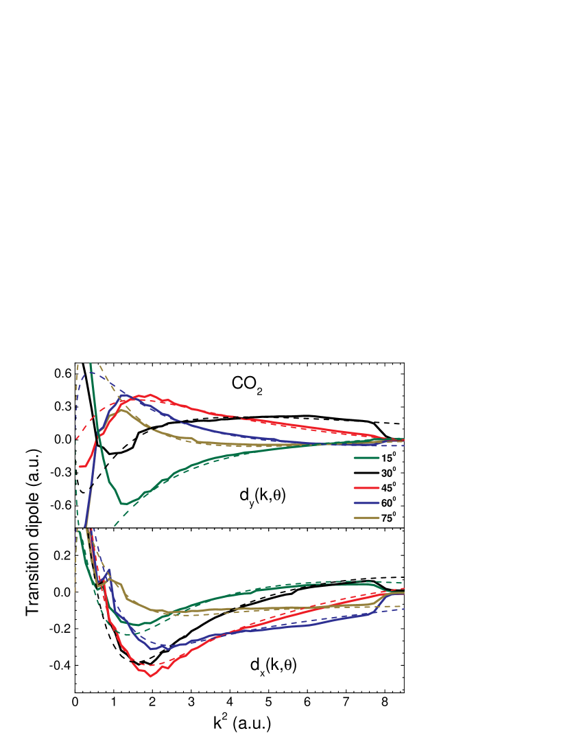
Figure 1: The extracted transition dipoles of CO₂ (solid lines) in comparison with the theoretical ones (dash lines) for few different alignments, shown in the labels. The upper and lower panels are for the $y$ and $x$ components, respectively. A 30 fs (FWHM) laser pulse with peak intensity of $2\times 10^{14}$ W/cm² and wavelength of $1200$ nm is used.

In Fig. 1 we compare the dipole moments extracted by using Eq. (2) with the theoretical data for a few alignment angles shown on the label. Clearly, one can see that the extracted data compare quite well with the theoretical ones for a broad range of $k^{2}\in[1-8]$ a.u., or from harmonic orders H27 to H109. Note that we choose the long wavelength of $1200$ nm instead of $800$ nm in order to have a broader useful range of harmonics for the tomographic procedure, as has been suggested in [5]. With these extracted dipoles, we then use the Fourier slice theorem to calculate the HOMO wavefunction. The contour plot of the retrieved HOMO for the case of equilibrium CO₂ shown in Fig. 2(e) has a clear $\pi_{g}$ symmetry, which compares quite well with the theoretical contour plot shown in Fig. 2(b). The distance between the oxygen and carbon centers, estimated as half the distance between the peaks along $x$-axis, is $R^{*}=2.12$ au, is also in reasonable good agreement with the input $R_{0}=2.2$ au. Similarly, good agreements are found for the case of $R_{0}=1.61$ and $2.79$ au, shown in the upper and lower panels of Fig. 2, respectively. The retrieved distances are $R^{*}=1.71$ and $2.63$ au, respectively.

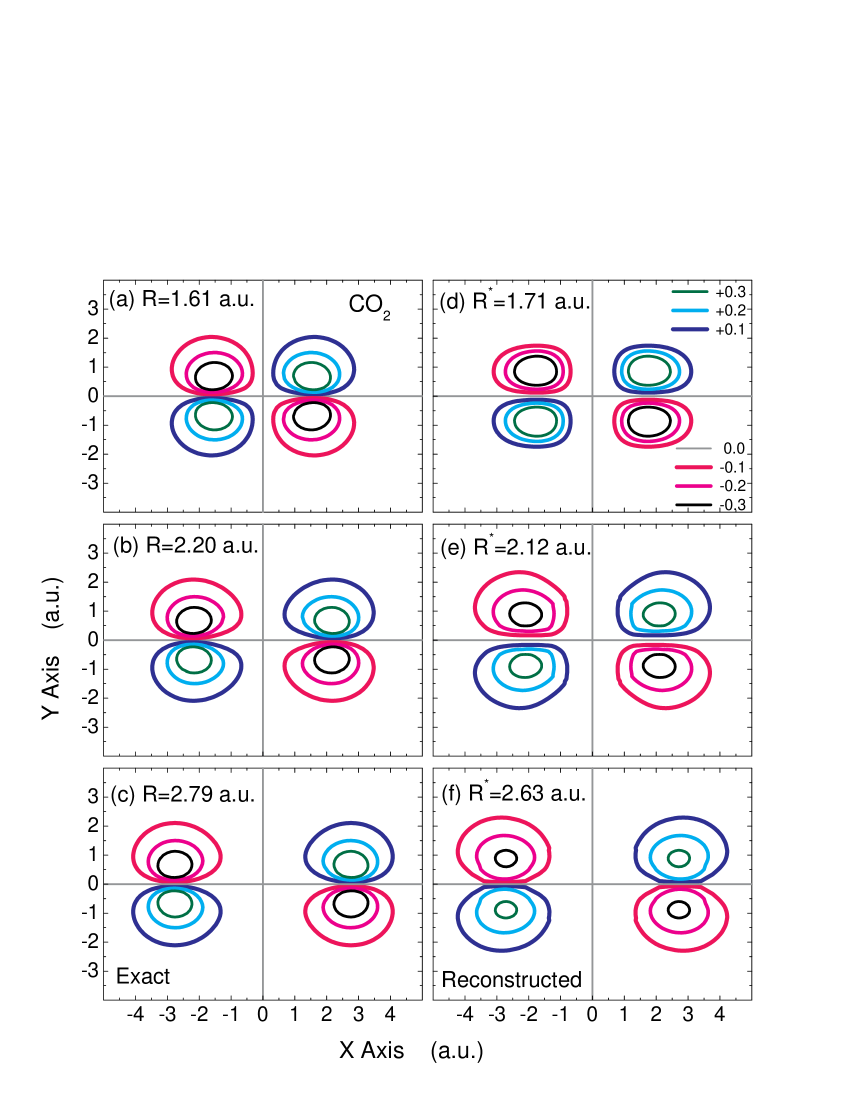
Figure 2: Contour plot of the retrieved HOMO wavefunctions of CO₂ [(d),(e),(f)], as compared to the exact ones [(a),(b),(c)] with the input internuclear distances (between oxygen and carbon centers) $R_{0}=1.61$, $2.2$, and $2.79$ a.u., respectively.

Figure 3: Polar plot of the ionization rates for CO₂, N₂ and O₂ from MO-ADK and SFA calculations, as functions of alignment angle between molecular axis and laser polarization direction. Laser pulse with peak intensity of $2\times 10^{14}$ W/cm², mean wavelength of $800$ nm and duration (FWHM) of 30 fs was used in calculations.

We found that in case of CO₂, the extracted dipoles agree better with the theoretical ones if the strong-field approximation is used to calculate ionization rate instead of the simple MO-ADK theory. It is interesting to note that recent measurements by the NRC group [13] also showed the alignment dependence of the ionization rate for CO₂ deviated significantly from the prediction by the MO-ADK theory. On the other hand, the MO-ADK predictions for N₂ and O₂ appear to be in very good agreement with the SFA results and with experiments [13, 14, 15]. In Fig. 3, we compare the CO₂ ionization rates from MO-ADK theory (blue line) and SFA (red line), plotted as function of the alignment angle. A laser with peak intensity of $2\times 10^{14}$ W/cm², mean wavelength of $800$ nm and duration (FWHM) of $30$ fs is used. The MO-ADK rate peaks near $30^{\circ}$, which is in agreement with results deduced from measured double ionization of CO₂ [16]. For MO-ADK calculations, we use the values of the coefficients $C_{l}$ as suggested in [17]. The SFA rate for CO₂ is quite similar in shape to that from O₂, but with the peak shifted to about $37^{\circ}$. This result appears to be in a better agreement with the NRC measurements, which show very narrow peak near $45^{\circ}$. The nature of the discrepancies between the two theories and with experiments are not clear so far. We note, however, that the good retrieval results by the tomographic procedure with the SFA theory for the ionization rates is likely due to the fact that the SFA model was also used to generate the HHG data. For completeness, we show the comparison between SFA and MO-ADK theories in case of N₂ and O₂, in Fig. 3(b) and (c), respectively. Clearly, the two theories agree quite well here.

3.2 Fitting procedure for extracting internuclear distances in case of fixed alignments

Now we discuss the results from the fitting procedure, described in Sec. 2.2. The success of the fitting procedure for extracting internuclear distances $R_{0}$ requires that HHG spectra be sensitive to this parameter. In Fig. 4(a) we show the calculated HHG from single N₂ molecules by a 30 fs laser pulse of wavelength of 800 nm and peak intensity of $2\times 10^{14}$ W/cm². The molecule is assumed to be aligned at $\theta=0^{\circ}$ with respect to the laser’s polarization axis. The known equilibrium distance for N₂ is $2.09$ a.u. We also show the HHG spectra with inputs $R_{0}=1.84$ and 2.27 a.u., amounting to about $10\%$ decrease or increase from the equilibrium distance, respectively. In Fig. 4(a) one can see that the HHG spectra for the three distances are quite distinguishable. The noticeable minimum for each $R_{0}$ moves to lower HHG order as $R_{0}$ is increased. In Fig. 4(b) we show that an introduction of $30\%$ or $60\%$ “experimental” errors to the data from $R_{0}=2.09$ a.u. does not show noticeable difference as compared to the actually calculated spectra. This comparison sheds light that the retrieval of $R_{0}$ should be relatively straightforward.

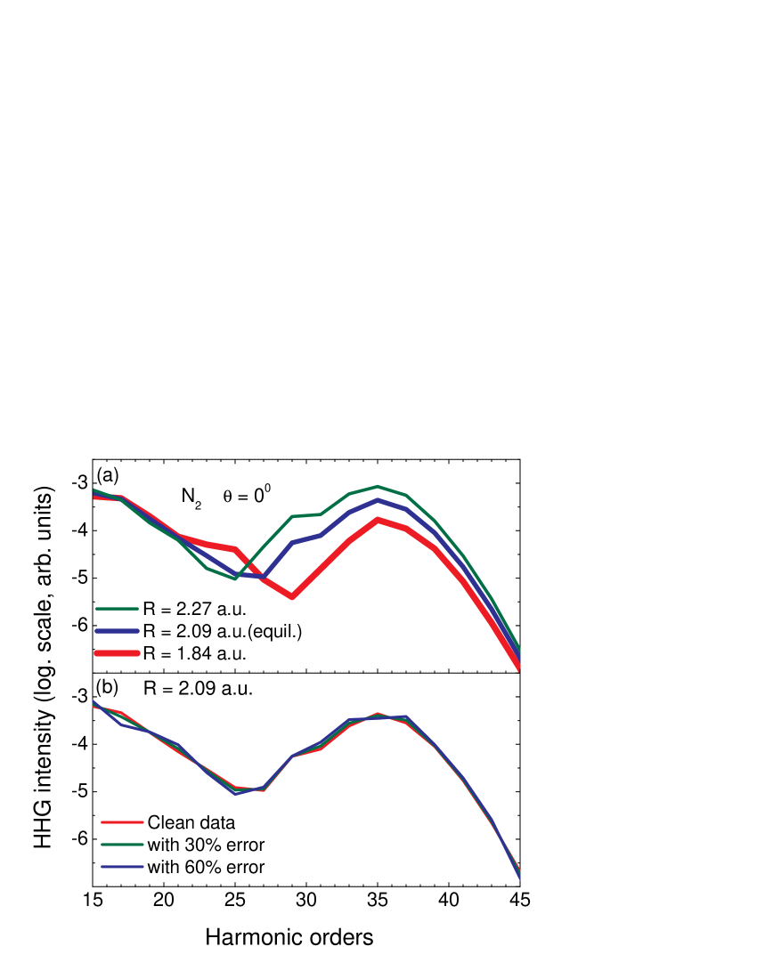
Figure 4: (a) HHG from N₂ with different internuclear distances $R_{0}=2.27$ (green line), $2.09$ (blue line), and $1.84$ (red line) calculated with fixed alignment angle $\theta=0^{\circ}$. (b) HHG from N₂ in equilibrium internuclear distance ($R_{0}=2.09$ au) with random “experimental” errors of $30\%$ (green line) and $60\%$ (blue line) at each harmonic.

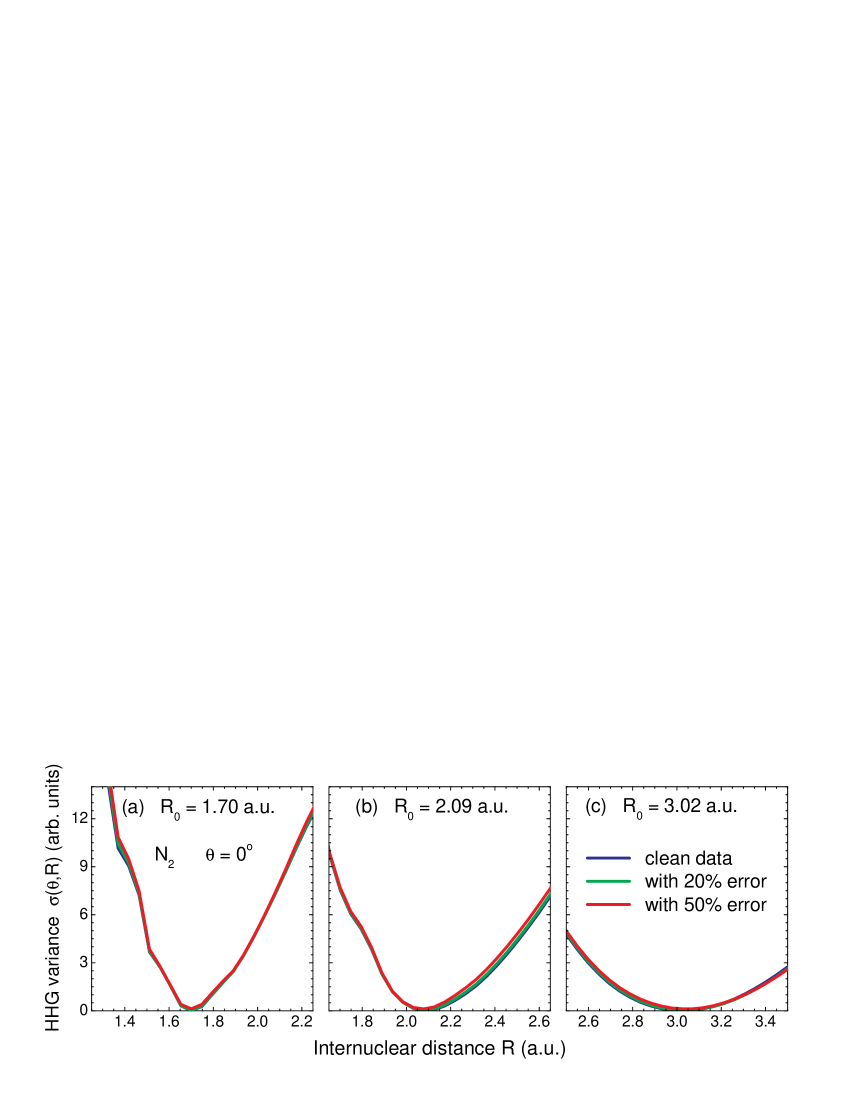
Figure 5: Variance of the HHG from N₂ for $R$ chosen near the input $R_{0}$ for the three different inputs $R_{0}=1.70$, $2.09$ (equilibrium) and $3.02$ a.u.

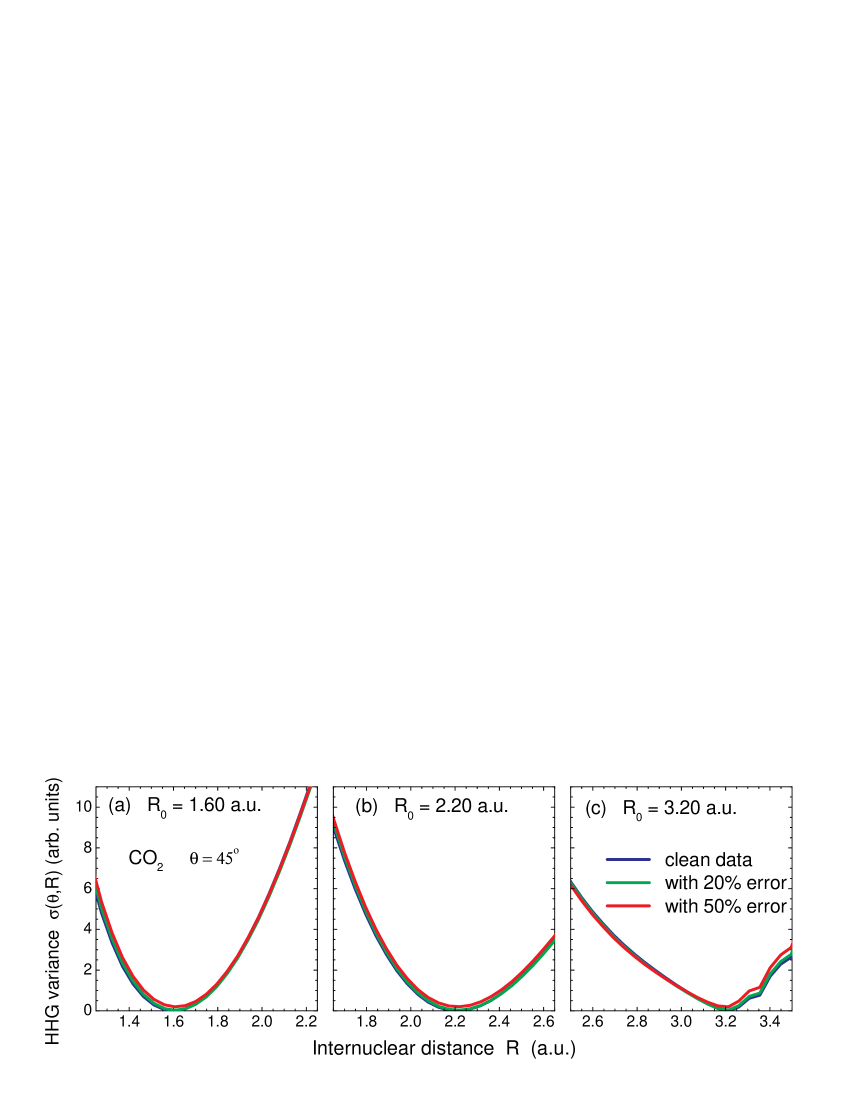
Figure 6: Same as Fig. 5, but for CO₂ with inputs $R_{0}=1.6$, $2.2$ (equilibrium) and $3.2$ a.u.

In Fig. 5, we show the variance as a function of internuclear distance, calculated by using Eq. (3), for each test case of N₂ with input $R_{0}=1.7,$ $2.09$, and $3.0$ au. Clearly the minimum in each case occurs near the input $R_{0}$, meaning that the value of the input internuclear separation can indeed be extracted with this simple fitting procedure. In the calculations shown in Fig. 5, we use the range of HHG in the plateau region, from H15-H45 for the alignment angle $\theta=0^{\circ}$. Similar results for CO₂ are shown in Fig. 6 using the same laser parameters, but for $\theta=45^{\circ}$. Again, the position of the minimum in each case matches closely to the input internuclear distance (between oxygen and carbon centers) of $R_{0}=1.6$, $2.2$, and $3.2$ a.u. Note that, in these calculations, only harmonics with parallel polarization are used. For the tomographic procedure, strictly speaking, one needs to know both components. We have tested the results by using different alignment angles and different ranges of harmonics and the retrieved internuclear distances are all very close to the input ones. Note that the accuracy of the retrieved internuclear distance can also be checked by using lasers of different wavelength or intensity.

3.3 Fitting in case of isotropic molecular distributions

The above fitting procedure has been applied to molecules fixed in space. At finite temperature, molecules can only be partially aligned or oriented. The above procedure can be generalized to these partially aligned molecules. Since only the internuclear distances are extracted, the fitting procedure can also be applied to molecules that are isotropically distributed. To illustrate the method, in this paper we assume that experimental HHG spectra from such isotropically distributed molecules are produced fully in phase so that the HHG amplitudes are added coherently.

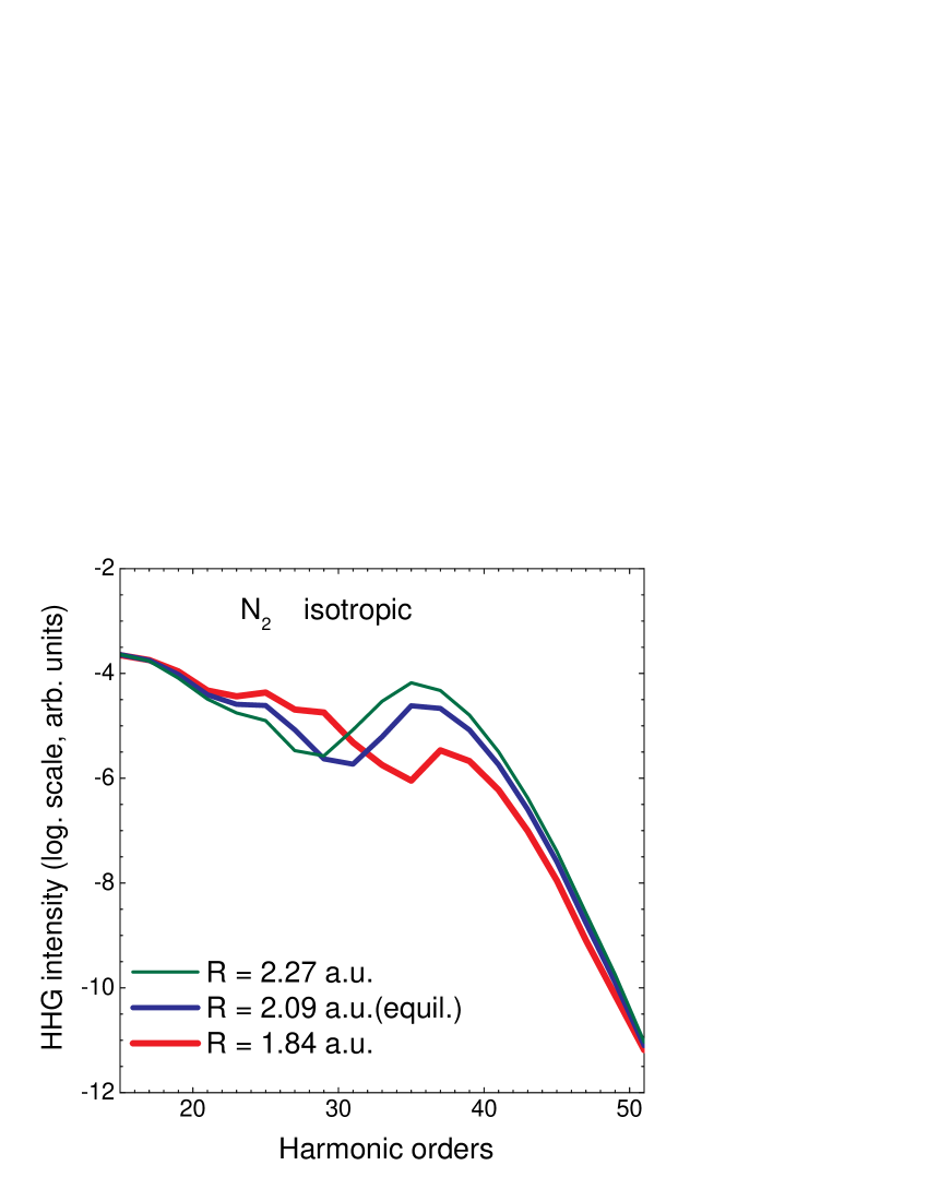
Figure 7: Same as Fig. 4(a), but for isotropically distributed molecular N₂. Such data can be used to retrieve $R_{0}$ using the fitting procedure.

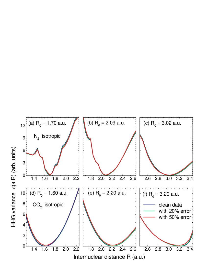
Figure 8: (a),(b), and (c): Variance of the HHG from N₂ for $R$ near the input $R_{0}=1.70$, $2.09$, and $3.02$ a.u., respectively, for the case of isotropic distribution. (d), (e), and (f): Same as (a), but for CO₂ near $R_{0}=1.60$, $2.20$, and $3.20$ a.u., respectively.

In Fig. 7, we show the calculated HHG spectra for such isotropically distributed N₂ molecules at $R_{0}=1.84$, $2.09$, and $2.27$ a.u. Note that the pronounced minima in the spectra can still be seen clearly, although their positions are moved to somewhat higher harmonics, compared to the case of $\theta=0^{\circ}$, shown in Fig. 4(a). This is not surprising since the HHG yield for small $\theta$ is dominant. Using the same fitting procedure [Eq. (3)], we confirmed that the $R_{0}$ can be extracted with similar accuracy. Typical results are presented in Fig. 8(a) and (b) for N₂ and CO₂, respectively, for few inputs $R$. Thus for simple systems, the internuclear distance can be extracted from the HHG yields even if the molecules are not aligned.

3.4 Fitting to transition dipoles

The above results establish the basic framework for the fitting procedure. The method is formulated in a general form and could easily be changed to tailor with modifications and extensions. We now discuss the results from the fitting to the transition dipoles. In Fig. 9 we show variance $\sigma(\theta,R)$ for transition dipole of O₂ with the input internuclear distance of $R_{0}=2.29$ a.u. and alignment angle of $45^{\circ}$. The fitting equation (4) is used, with the harmonics generated by the laser with peak intensity of $2\times 10^{14}$ W/cm², wavelength of $800$ nm and duration of $30$ fs. The summation in Eq. (4) was carried out for the range H19-H43. That corresponds to the fitting range $k^{2}\in[1.28-4.0]$ a.u. The “experimental” transition dipoles were calculated using Eq. (2), using Xe as the reference atom. For each guess of the internuclear distance, the theoretical dipoles are calculated within the plane-wave approximation for the continuum electron, in order to be consistent with the SFA model for the HHG used here. As can be seen from the figure, the minimum position indeed agrees well with the input $R_{0}$. The data are shown for the fitting to the $d_{x}$ component of the dipole (in the molecular frame). The fitting to $d_{y}$ component leads to similar result. In fact, the minimum positions are very close to the input $R_{0}=2.29$ a.u. for all other alignment angles we tried.

Figure 9: Variance of the transition dipole for O₂ for $R$ near the input $R_{0}=2.29$ au.

Note that dipole moments were used directly in extracting the structural information in this approach, similar to the method used in the tomographic procedure. Once again, since only the internuclear distance is retrieved, the method is much easier to implement experimentally in time-resolved measurements. In real situation, in order to fit with experimental data, exact transition dipoles calculated by using scattering waves should be used. This does not pose additional difficulties within the fitting method. In this connection we note here that this extension (beyond the plane-wave approximation) would make the simple tomographic procedure inapplicable, as the Fourier slice theorem cannot be used directly.

4 Conclusions and Perspective

In this paper we have shown that the simple iterative fitting procedure is very efficient for extracting the internuclear separations from the high-order harmonics generated by infrared lasers. This method, in combination with the available quantum chemistry codes, can be made a very powerful tool for exploring the time-resolved structural changes in a chemical transformation. The procedure is much simpler than the tomographic method suggested by Itatani et al [4]. It also does not rely on the assumptions made in that paper.

For the iterative method to work, an adequate theory for calculating high-order harmonics from molecules has to be available and the calculations be very efficient. In the present work, this theory is available in the form of strong field approximation (SFA). However, the SFA is an approximate theory and the HHG spectra calculated using SFA is not expected to be in agreement with the experimental data. In principle, HHG spectra can be calculated by solving the time-dependent Schrödinger equation. However, such calculations for molecular targets in arbitrary alignment is very time consuming and the results are likely not of sufficient accuracy in general. Thus in the near future, even for the simple molecules such as N₂, O₂ and CO₂ studied in the present paper, the iterative method based on Eq. (3) is not practical. Fortunately, an alternative route is possible. Very recently it has been shown by Morishita et al [18] and Le et al [19] that Eq. (1) is applicable to accurate HHG spectra of atoms generated by infrared lasers. The establishment of validity of Eq. (1) in this case was based on accurate HHG spectra obtained by solving the time-dependent Schrödinger equation for atoms in intense laser fields and for transition dipole matrix elements calculated using accurate scattering waves, i.e., accurate wavefunctions of electrons in the continuum. We anticipate that HHG spectra from molecular targets obtained from accurate theory (for H${}_{2}^{+}$ target this has been shown in Le et al [20]) or from experiment can also be factored out in the form of Eq. (1) where the transition dipole matrix elements $d(\omega,\theta)$ are calculated using scattering waves. Note that $d(\omega,\theta)$ is the same transition dipole matrix element calculated in the study of photoionization cross sections of molecules.

Unlike the nonlinear laser-molecule interactions, photoionization is a linear process, and they can be calculated with much less effort. In particular, for our purpose, we do not need high-precision photoabsorption cross sections in a narrow energy region such as those measured with synchrotron radiation, but rather moderately accurate dipole matrix elements over a broad photon energy range. Thus simpler calculations based on the one-electron model along the line developed by Tonzani [21] is likely adequate for this purpose. Clearly further development along this line requires the input of experimental data in order to demonstrate the actual working of the iterative method. If the method is established, it would be rather straightforward to extend the method to carry out the time-resolved chemical imaging with few-cycle infrared laser pulses, achieving temporal resolutions down to a few femtoseconds, depending on the pulse durations of the probe pulses used.

References

References

- [1] Zewail A H 2000 J. Phys. Chem. A 104 5660
- [2] Ihee H, Lobastov V A, Gomez U M, Goodson B M, Srinivasan M, Ruan C Y and Zewail A H 2001 Science 291 458
- [3] Lein M 2007 J. Phys. B 40 R135
- [4] Itatani J, Levesque J, Zeidler D, Niikura H, Pepen H, Kieffer J C, Corkum P B and Villeneuve D M 2004 Nature (London) 432 867
- [5] Le V H, Le A T, Xie R H and Lin C D 2007 Phys. Rev. A 76 013414
- [6] Tong X M, Zhao Z and Lin C D 2002 Phys. Rev. A 66 033402
- [7] Frisch M J et al 2003 GAUSSIAN 03, revision C.02 (Gaussian, Inc., Pittsburgh, PA)
- [8] Schmidt M W et al 1993 J. Comput. Chem. 14 1347
- [9] Lewenstein M, Balcou Ph, Ivanov M Yu, L’Huillier A and Corkum P B 1994 Phys. Rev. A 49 2117
- [10] Zhou X X, Tong X M, Zhao Z X and Lin C D 2005 Phys. Rev. A 71 061801(R)
- [11] Le A T, Tong X M and Lin C D 2006 Phys. Rev. A 73 041402(R)
- [12] Levesque J, Mairesse Y, Dudovich N, Pepin H, Kieffer J C, Corkum P B and Villeneuve D M 2007 Phys. Rev. Lett. 99 243001
- [13] Pavicic D, Lee K F, Rayner D M, Corkum P B and Villeneuve D M 2007 Phys. Rev. Lett. 98 243001
- [14] Litvinyuk I V, Lee K F, Dooley P W, Rayner D M, Villeneuve D M and Corkum P B 2003 Phys. Rev. Lett. 90 233003
- [15] Alnaser A S, Voss S, Tong X M, Maharjan C M, Ranitovic P, Ulrich B, Osipov T, Shan B, Chang Z and Cocke C L 2004 Phys. Rev. Lett. 93 113003
- [16] Alnaser A S, Maharjan C M, Tong X M, Ulrich B, Ranitovic P, Shan B, Chang Z, Lin C D, Cocke C L and Litvinyuk I V 2005 Phys. Rev. A 71 031403(R)
- [17] Le A T, Tong X M and Lin C D 2007 J. Mod. Optics 54 967
- [18] Morishita T, Le A T, Chen Z and Lin C D 2008 Phys. Rev. Lett. 100 013903
- [19] Le A T, Morishita T and Lin C D 2008 submitted to Phys. Rev. Lett.
- [20] Le A T et al (in preparation)
- [21] Tonzani S 2007 Comput. Phys. Comm. 176 146