The Role of Bound States in Time-Dependent Quantum Transport

Abstract

Charge transport through a nanoscale junction coupled to two macroscopic electrodes is investigated for the situation when bound states are present. We provide numerical evidence that bound states give rise to persistent, non-decaying current oscillations in the junction. We also show that the amplitude of these oscillations can exhibit a strong dependence on the history of the applied potential as well as on the initial equilibrium configuration. Our simulations allow for a quantitative investigation of several transient features. We also discuss the existence of different time-scales and address their microscopic origin.

I Introduction

In order to describe electronic transport through mesoscopic or nanoscopic devices, a quantum description of transport is essential. A seminal quantum theory of transport is the Landauer-Büttiker formalism,Landauer (1957); Büttiker (1986) which expresses the conductance of a device in terms of the quantum-mechanical transmittance of (non-interacting) electrons at the Fermi energy.

In recent years and spurred by experimental progress in transport measurements through single molecules,M.A. Reed et al. (1997) the Landauer-Büttiker formalism has been combined N.D. Lang (1995); Hirose and Tsukada (1995); J.M. Seminario et al. (1998); Taylor et al. (2001); Palacios et al. (2001); Xue et al. (2002); Brandbyge et al. (2002); Evers et al. (2004); Faleev et al. (2005) with (static) density functional theory which allows to take the atomistic structure of both the molecule and the contacts into account. For a recent critical review of this methodology, the reader is referred to Ref. Koentopp et al., 2008.

The Landauer-Büttiker formalism focusses on the description of steady-state transport and assumes that for a system which is driven out of equilibrium by a dc bias, a dc current will eventually develop, which means that the dynamical formation of the steady state is not proved but rather taken for granted. The question how the system dynamically reaches a steady state has been investigated both numericallyKurth et al. (2005); Bushong et al. (2005); Sanchez et al. (2006); Sai et al. (2007) and theoretically.Cini (1980); Stefanucci and C.-O. Almbladh (2004a) Using non-equilibrium Green functions (NEGF) techniques it has been shownStefanucci and C.-O. Almbladh (2004a) that the total current (and density) approaches a steady value provided the local density of states is smooth in the device region. Such value is 1) in agreement with the Landauer formula and 2) independent of the initial equilibrium configuration and the history of the applied bias. For a steady state to develop the condition on the local density of states excludes the presence of bound states. Recently, the inclusion of bound states in time-dependent quantum transport has been studied in Ref. Dhar and Sen, 2006 and further been addressed in subsequent work.Stefanucci (2007) There it is demonstrated that if the dc biased Hamiltonian supports two or more bound states, the long-time limit of the current consists of two terms: a steady-state contribution given by the Landauer formula and an additional, dynamical contribution responsible for undamped current oscillations. The frequencies of these oscillations are given by the differences between two bound-state energies and, interestingly, the amplitudes depend on both the initial state and history of the time-dependent perturbation.

In the present work, the history as well as the initial-state dependence of the dynamical part of the current is investigated numerically in detail. As a tool for our numerical calculations we use a recently developed algorithm Kurth et al. (2005) which allows for the time propagation of quantum transport systems according to the Schrödinger equation.

The paper is organized as follows. In Section II we summarize the results of Ref. Stefanucci, 2007 which are relevant for the discussion of our findings and we briefly describe the central ideas of the time-propagation algorithm. In Section III we present our numerical results which not only confirm the existence of the undamped current oscillations but also allow to identify additional internal transitions contributing to the transient behavior of the driven system. We investigate the dependence of the current oscillations on various parameters and initial conditions and provide theoretical explanations of the observed behavior. Finally, we recapitulate our main results in Section IV.

II Two Approaches to Time-Dependent Transport

In this Section we briefly describe two alternative approaches to time-dependent transport in a typical electrode-device-electrode geometry: non-equilibrium Green functions (NEGF) and direct solution of the time-dependent Schrödinger equation. As was already pointed out within the former approach,Dhar and Sen (2006); Stefanucci (2007) quantum transport in systems of non-interacting electrons exhibits persistent current- (and density-) oscillations if two or more bound states are present in the biased system. Here, we use the latter approach to address several issues about such bound-state oscillations. A particularly interesting feature of them is the fact that their amplitude depends on the entire time evolution as the system is driven out of equilibrium (memory effects).

II.1 Non-equilibrium Green functions

We consider a quantum system of non-interacting electrons which consists of a central device (e.g., a quantum point contact or a single molecule plus a few atomic layers of the left and right electrodes) and two semi-infinite reservoirs (left and right electrodes). As initial state we use the one proposed by Cini:Cini (1980) all parts of the system, i.e., left lead (region $L$), central device (region $C$) and right lead (region $R$), are initially (at $t\leq 0$) connected and in a well defined equilibrium configuration with a unique temperature and chemical potential (thermodynamic consistency). In this initial state, the charge density of the electrodes is perfectly balanced and no current flows through the junction.

For non-interacting electrons at zero temperature, the initial state is a Slater determinant of eigenstates of the entire contacted system with eigenenergies smaller than the Fermi energy. At time $t>0$ the system is driven out of equilibrium by exposing it to an external time-dependent potential which is local in time and space. For example, we may switch on an electromotive force in such a way that the potential drop is entirely limited to the central region. The boundaries of the open quantum system are chosen in a way that the density outside the region $C$ is accurately described by an equilibrium bulk density. The time-dependent perturbation may cause a current flow through the device. The total current from region $\alpha=L,R$ can be calculated from time derivative of the total number of particles in $\alpha$:

$$I_{\alpha}(t)=-e\int_{\alpha}{\rm d}\mbox{\boldmath$r$}\;\frac{{\rm d}}{{\rm d}t}n(\mbox{\boldmath$r$},t),\quad\alpha=L,R,$$ (1)

where $n(\mbox{\boldmath$r$},t)$ is the time-dependent electron density and the space integral extends over region $\alpha$ ($e$ is the electron charge). Assuming no direct coupling between the left and right electrodes, the single-particle Hamiltonian of the entire, contacted system can be written as:

$$\mbox{\boldmath$H$}(t)=\left[\begin{array}[]{ccc}\mbox{\boldmath$H$}_{LL}(t)&\mbox{\boldmath$H$}_{LC}&0\\ \mbox{\boldmath$H$}_{CL}&\mbox{\boldmath$H$}_{CC}(t)&\mbox{\boldmath$H$}_{CR}\\ 0&\mbox{\boldmath$H$}_{RC}&\mbox{\boldmath$H$}_{RR}(t)\end{array}\right].$$ (2)

The diagonal blocks of the above matrix are obtained by projecting the full Hamiltonian $H$ onto the corresponding region. The off-diagonal blocks in Eq. (2) account for the coupling between the device region $C$ and the leads and, for simplicity, we assume them to be time-independent. For instance, in a real-space representation using a finite-difference discretization of the kinetic energy, the off-diagonal elements of $H$ are simply given by the off-diagonal elements of the kinetic energy operator. (Model systems with time-dependent couplings were studied, e.g., in Ref. Moldoveanu et al., 2007.)

One way to deal with non-equilibrium problems is provided by the NEGF theory. From the equation of motion of the Keldysh-Green function one can rewrite the current $I_{\alpha}(t)$ of Eq. (1) in terms of the lesser Green function projected onto different subregions as:

$$I_{\alpha}(t)=2e{\rm Re}\,{\rm Tr}[\mathbf{G}_{C\alpha}^{<}(t,t)\mbox{\boldmath$H$}_{\alpha C}],$$ (3)

where ${\rm Tr}$ denotes the trace over a complete set of states in the central region. The lesser Green function can be expressed Blandin et al. (1976); Cini (1980); Danielewicz (1984); Stefanucci and C.-O. Almbladh (2004b, a) in terms of retarded and advanced Green functions as

$$\mathbf{G}^{<}(t;t^{\prime})=\mathbf{G}^{R}(t;0)\mathbf{G}^{<}(0;0)\mathbf{G}^{A}(0;t^{\prime}).$$ (4)

The initial condition is $\mathbf{G}^{<}(0;0)=if(\mbox{\boldmath$H$}^{0})$ where $f(\omega)=(e^{\beta(\omega-\mu)}+1)^{-1}$ is the Fermi distribution function and $\mbox{\boldmath$H$}^{0}$ is the (time-independent) Hamiltonian for $t<0$.

It can be shown Stefanucci and C.-O. Almbladh (2004b) that in a dc biased system the total time-dependent current approaches a steady value provided the local density of states in region $C$ is smooth. In this case, the steady current is given by:

$$I_{L}^{(S)}=\lim_{t\to\infty}I_{\alpha}(t)=e\int\frac{d\omega}{2\pi}[f(\omega-U_{L}^{\infty})-f(\omega-U_{R}^{\infty})]T(\omega).$$ (5)

In the above equation $U_{\alpha}^{\infty}$ is the value approached by the bias in lead $\alpha$ when $t\to\infty$ and $T(\omega)={\rm Tr}[\mathbf{G}^{R}_{CC}(\omega)\mathbf{\Gamma}_{L}(\omega)\mathbf{G}^{A}_{CC}(\omega)\mathbf{\Gamma}_{R}(\omega)]$, where $\mathbf{\Gamma}_{\alpha}(\omega)=-2{\rm Im}[\mbox{\boldmath$\Sigma$}_{\alpha}^{R}(\omega)]$ and $\mathbf{G}^{R/A}_{CC}$ are the retarded and advanced Green functions projected in region $C$. $\mbox{\boldmath$\Sigma$}_{\alpha}^{R}(\omega)=\mbox{\boldmath$H$}_{C\alpha}\mbox{\boldmath$g$}^{R}_{\alpha\alpha}(\omega)\mbox{\boldmath$H$}_{\alpha C}$ is the embedding self energy with the retarded Green function of lead $\alpha$, $\mbox{\boldmath$g$}^{R}_{\alpha\alpha}(\omega)=\left(\omega-\mbox{\boldmath$H$}_{\alpha\alpha}^{0}-U^{\infty}_{\alpha}+i0^{+}\right)^{-1}$ . The steady current does not depend on the initial Hamiltonian (the memory of different initial conditions is completely washed out) and is also independent of the history of the applied bias (memory-loss theorem).Stefanucci and C.-O. Almbladh (2004a)

The above scenario changes drastically if the Hamiltonian $\mbox{\boldmath$H$}^{\infty}:=\lim_{t\to\infty}\mbox{\boldmath$H$}(t)$ has two or more bound eigenstates. In this case the long-time limit of the current has two contributions:Stefanucci (2007)

$$\lim_{t\rightarrow\infty}I_{\alpha}(t)=I_{\alpha}^{(S)}+I_{\alpha}^{(D)}(t)\;.$$ (6)

In addition to the steady-state contribution $I_{\alpha}^{(S)}$ given by Eq. (5) one finds a dynamical, explicitly time-dependent contribution $I_{\alpha}^{(D)}$ which can be written as

$$I_{\alpha}^{(D)}(t)=2e\sum_{b,b^{\prime}}{f_{b,b^{\prime}}\Lambda_{b,b^{\prime}}^{(\alpha)}\sin[(\epsilon_{b}^{\infty}-\epsilon_{b^{\prime}}^{\infty})t]}.$$ (7)

In Eq. (7) the summation is over all bound states of the final Hamiltonian $\mbox{\boldmath$H$}^{\infty}$ and $I_{\alpha}^{(D)}$ oscillates with frequencies given by the differences of the bound-state eigenenergies. The quantities ${\Lambda}_{b,b^{\prime}}$ and $f_{b,b^{\prime}}$ are defined according to

$${\Lambda}_{b,b^{\prime}}^{(\alpha)}={\rm Tr}_{C}\left[|\psi_{bC}^{\infty}\rangle\langle\psi_{b^{\prime}C}^{\infty}|\mbox{\boldmath$\Sigma$}_{\alpha}^{A}{(\epsilon_{b}^{\prime})}\right],$$ (8)

and

$$f_{b,b^{\prime}}=\langle\psi^{\prime}_{b}|f(\mbox{\boldmath$H$}^{0})|\psi^{\prime}_{b^{\prime}}\rangle\;.$$ (9)

The state $|\psi_{bC}^{\infty}\rangle$ is the projection of the bound eigenstate $|\psi_{b}^{\infty}\rangle$ of the biased Hamiltonian $\mbox{\boldmath$H$}^{\infty}$ onto the central region. The state $|\psi^{\prime}_{b}\rangle$ is related to $|\psi_{b}^{\infty}\rangle$ by a unitary transformation:

$$\left[\begin{array}[]{c}|\psi^{\prime}_{bL}\rangle\\ |\psi^{\prime}_{bC}\rangle\\ |\psi^{\prime}_{bR}\rangle\end{array}\right]=\left[\begin{array}[]{ccc}e^{i\Delta^{\infty}_{L}}\mbox{\boldmath$1$}_{L}&0&0\\ 0&\mbox{\boldmath$M$}_{C}&0\\ 0&0&e^{i\Delta^{\infty}_{R}}\mbox{\boldmath$1$}_{R}\end{array}\right]\left[\begin{array}[]{c}|\psi_{bL}^{\infty}\rangle\\ |\psi_{bC}^{\infty}\rangle\\ |\psi_{bR}^{\infty}\rangle\end{array}\right],$$ (10)

with

$$\Delta^{\infty}_{\alpha}=\lim_{t\rightarrow\infty}\int_{0}^{t}{\rm d}t^{\prime}(U_{\alpha}\left(t^{\prime}\right)-U_{\alpha}^{\infty}),$$ (11)

$\mbox{\boldmath$M$}_{C}$ a unitary “memory matrix” with the same dimension as the number of degrees of freedom employed to describe region $C$ and $\mbox{\boldmath$1$}_{\alpha}$ the identity matrix projected onto region $\alpha=L,R$ . The memory matrix depends on the history of the time-dependent perturbation and is defined through the equation below

$$\lim_{t\rightarrow\infty}\mathbf{G}^{A}_{CC}(0;t)=\mbox{\boldmath$M$}_{C}\lim_{t\rightarrow\infty}\bar{\mathbf{G}}^{A}_{CC}(0;t),$$ (12)

where $\bar{\mathbf{G}}^{A}_{CC}(0;t)$ is the projection onto region $C$ of the advanced Green function $\bar{\mathbf{G}}^{A}(0;t)=i\exp(i\mbox{\boldmath$H$}^{\infty}t)$.

Few remarks about the central result in Eq. (6) are in order. First, we wish to emphasize again that no steady-state current develops if the biased Hamiltonian $\mbox{\boldmath$H$}^{\infty}$ has bound eigenstates. The current oscillations given by Eq. (7) are persistent, i.e., they do not decay in time. Second, in contrast to the case without bound states, the asymptotic current $I_{\alpha}(t)$ depends both on the initial equilibrium configuration and history of the applied bias and gate voltage through the coefficients $f_{b,b^{\prime}}$ of Eq. (9). For sudden switching of the bias and gate voltage $\Delta^{\infty}_{\alpha}=0$ and $\mbox{\boldmath$M$}_{C}={\mbox{\boldmath$1$}}_{C}$ (${\mbox{\boldmath$1$}}_{C}$ being the identity matrix projected onto region $C$) and the matrix in Eq. (10) reduces to the identity matrix. On the contrary, different switching processes yield different memory matrices and hence different amplitudes of the current oscillations, see Section III for a detailed study of the history dependence. Third, the NEGF formalism described in this Section can be combined with Time-Dependent Density Functional Theory Runge and E.K.U. Gross (1984); E.K.U. Gross and Kohn (1990) (TDDFT) to include exchange and correlation effects in the calculated density and current. In this theory the steady-state assumption is consistent with the TDDFT equation for the total current provided the density of states in region $C$ is a smooth function.Stefanucci and C.-O. Almbladh (2004b) On the contrary, the presence of bound-states in the biased Hamiltonian is not compatible with a steady current.Stefanucci (2007) This result opens up the possibility of having oscillatory solutions even for constant biases and may change substantially the standard steady-state picture already at the level of exchange-correlation functionals which are local or semi-local in time. On one hand, the oscillations of the effective potential in region $C$ give rise to new conductive channels, an effect that cannot be captured in any static approach. On the other hand, the asymptotic ($t\rightarrow\infty$) density depends on the occupation coefficients $f_{b,b}$ which in turn depend on the history of the TDDFT potential. Thus, history-dependent effects might be observed even at the level of the adiabatic local density approximation. Finally we emphasize that the above conclusions are not limited to TDDFT but also apply to any other single-particle theory of electrons such as, e.g., Hartree-Fock theory. Similarly, they also apply to a single-electron theory of coupled electronic and nuclear motion where the time evolution of the nuclei is treated in the Ehrenfest approximation and thus the potential acting on the electrons depends parametrically on the (time-dependent) nuclear coordinates. In this latter case the presence of a self-consistent oscillatory solution in a Holstein wire connected to one-dimensional non-interacting leads was observed in Ref. Verdozzi et al., 2006.

II.2 Direct propagation of the time-dependent Schrödinger equation

Calculating the time-dependent current in terms of the Green function projected onto the central region amounts to solving either the Keldysh-Dyson integral equationsZhu et al. (2005); Maciejko et al. (2006) or the integro-differential Kadanoff-Baym equations.L.P. Kadanoff and Baym (1962); N.E. Dahlen and R. van Leeuwen (2007) In this work we use an alternative approach which is based on solving the time-dependent Schrödinger equation for the initially occupied one-particle states.Kurth et al. (2005) An advantage of the latter approach over the former ones is that the wave-functions depend only on one time argument as opposed to the double time dependence of the Green function. This algorithm has recently also been used to study electron pumping by direct time propagation Stefanucci et al. .

For non-interacting electrons at zero temperature the total current from region $\alpha$ of Eq. (1) can alternatively be expressed as a surface integral

$$I_{\alpha}(t)=-e\sum_{\rm occ}\int_{S_{\alpha}}{\rm d}\sigma\,\hat{{\bf n}}\cdot{\rm Im}\left[\psi_{n}^{\ast}(\mbox{\boldmath$r$},t)\mbox{\boldmath$\nabla$}\psi_{n}(\mbox{\boldmath$r$},t)\right],$$ (13)

where $\hat{{\bf n}}$ is the unit vector perpendicular to the surface element ${\rm d}\sigma$, the surface $S_{\alpha}$ is perpendicular to the longitudinal geometry of our system and $\psi_{n}(\mbox{\boldmath$r$},0)$ are the eigenstates of $\mbox{\boldmath$H$}(t<0)$. The electrode-junction-electrode system is infinitely extended and non-periodic. In practice, of course, we can only deal with finite systems and therefore we only propagate the initial wavefuction projected onto the central region $C$. The presence of the leads is taken into account by applying the correct boundary conditions. It is worth to note that even for interacting electrons one can use Eq. (13) to compute the current through the junction if the single-particle orbitals $\psi_{n}(\mbox{\boldmath$r$},t)$ are the Kohn-Sham orbitals of time-dependent density functional theory.

For a description of the algorithm proposed in Ref. Kurth et al., 2005, it is convenient to write $\mbox{\boldmath$H$}_{\alpha\alpha}(t)$, with $\alpha=L,R$ , as the sum of a term $\mbox{\boldmath$H$}^{0}_{\alpha\alpha}=\mbox{\boldmath$H$}_{\alpha\alpha}(0)$ which is constant in time and another term $\mbox{\boldmath$U$}_{\alpha}(t)$ which may be explicitly time-dependent, $\mbox{\boldmath$H$}_{\alpha\alpha}(t)=\mbox{\boldmath$H$}^{0}_{\alpha\alpha}+\mbox{\boldmath$U$}_{\alpha}(t)$. In configuration space $\mbox{\boldmath$U$}_{\alpha}(t)$ is diagonal at any time $t$ since the potential is local in space. Furthermore, the diagonal elements $U_{\alpha}(\mbox{\boldmath$r$},t)$ are spatially constant for metallic electrodes. Thus, $\mbox{\boldmath$U$}_{\alpha}(t)=U_{\alpha}(t){\mbox{\boldmath$1$}}_{\alpha}$ and $U_{L}(t)-U_{R}(t)$ is the total potential drop across the junction. The total Hamiltonian is $\mbox{\boldmath$H$}(t)=\tilde{\mbox{\boldmath$H$}}(t)+\mbox{\boldmath$U$}(t)$ with

$$\tilde{\mbox{\boldmath$H$}}(t)=\left[\begin{array}[]{ccc}\mbox{\boldmath$H$}^{0}_{LL}&\mbox{\boldmath$H$}_{LC}&0\\ \mbox{\boldmath$H$}_{CL}&\mbox{\boldmath$H$}_{CC}(t)&\mbox{\boldmath$H$}_{CR}\\ 0&\mbox{\boldmath$H$}_{RC}&\mbox{\boldmath$H$}^{0}_{RR}\end{array}\right]$$

and

$$\mbox{\boldmath$U$}(t)=\left[\begin{array}[]{ccc}U_{L}(t){\mbox{\boldmath$1$}}_{L}&0&0\\ 0&0&0\\ 0&0&U_{R}(t){\mbox{\boldmath$1$}}_{R}\end{array}\right].$$ (14)

In this way, the only term in $\tilde{\mbox{\boldmath$H$}}(t)$ that depends on $t$ is $\mbox{\boldmath$H$}_{CC}(t)$. For any given initial one-particle state $|\psi(0)\rangle=|\psi^{(0)}\rangle$ we calculate $|\psi(t_{m}=m\Delta t)\rangle=|\psi^{(m)}\rangle$ by employing a generalized form of the Cayley method (atomic units are used throughout)

$$\left({\bf 1}+i\delta\tilde{\mbox{\boldmath$H$}}^{(m)}\right)\frac{{\bf 1}+i\frac{\delta}{2}\mbox{\boldmath$U$}^{(m)}}{{\bf 1}-i\frac{\delta}{2}\mbox{\boldmath$U$}^{(m)}}|\psi^{(m+1)}\rangle=$$

$$\left({\bf 1}-i\delta\tilde{\mbox{\boldmath$H$}}^{(m)}\right)\frac{{\bf 1}-i\frac{\delta}{2}\mbox{\boldmath$U$}^{(m)}}{{\bf 1}+i\frac{\delta}{2}\mbox{\boldmath$U$}^{(m)}}|\psi^{(m)}\rangle,$$ (15)

with $\tilde{\mbox{\boldmath$H$}}^{(m)}=\frac{1}{2}[\tilde{\mbox{\boldmath$H$}}(t_{m+1})+\tilde{\mbox{\boldmath$H$}}(t_{m})]$, $\mbox{\boldmath$U$}^{(m)}=\frac{1}{2}[\mbox{\boldmath$U$}(t_{m+1})+\mbox{\boldmath$U$}(t_{m})]$ and $\delta=\Delta t/2$. The above propagation scheme is unitary (norm conserving) and accurate to second-order in $\delta$. From Eq. (15) we can extract an equation for the time-evolved state in region $C$. After some algebra, one ends up with an equation which gives the wave function in region $C$ at time step $m+1$ in terms of the wave function in region $C$ at the previous time step and two additional terms (source and memory term):

$$|\psi_{C}^{(m+1)}\rangle=\frac{{\bf 1}_{C}-i\delta\mbox{\boldmath$H$}_{\rm eff}^{(m)}}{{\bf 1}_{C}+i\delta\mbox{\boldmath$H$}_{\rm eff}^{(m)}}|\psi_{C}^{(m)}\rangle+|S^{(m)}\rangle-|M^{(m)}\rangle.$$ (16)

The effective Hamiltonian $\mbox{\boldmath$H$}_{\rm eff}^{(m)}$ of region $C$ is defined according to $\mbox{\boldmath$H$}_{\rm eff}^{(m)}=\mbox{\boldmath$H$}_{CC}^{(m)}-i\delta\mbox{\boldmath$H$}_{CL}(1+i\delta\mbox{\boldmath$H$}^{0}_{LL})^{-1}\mbox{\boldmath$H$}_{LC}-i\delta\mbox{\boldmath$H$}_{CR}(1+i\delta\mbox{\boldmath$H$}^{0}_{RR})^{-1}\mbox{\boldmath$H$}_{RC}$, where $\mbox{\boldmath$H$}_{CC}^{(m)}=\frac{1}{2}[\mbox{\boldmath$H$}_{CC}(t_{m+1})+\mbox{\boldmath$H$}_{CC}(t_{m})]$. The source term $|S^{(m)}\rangle$ depends on the initial wavefunction in region $\alpha=L,R$ and reads

$$|S^{(m)}\rangle=-\frac{2i\delta}{1+i\delta\mbox{\boldmath$H$}_{\rm eff}^{(m)}}\sum_{\alpha=L,R}\frac{\Lambda_{\alpha}^{(m,0)}}{u_{\alpha}^{(m)}}\mbox{\boldmath$H$}_{C\alpha}$$

$$\times\frac{(1-i\delta\mbox{\boldmath$H$}_{\alpha\alpha})^{m}}{(1+i\delta\mbox{\boldmath$H$}_{\alpha\alpha})^{m+1}}|\psi_{\alpha}^{(0)}\rangle\;,$$ (17)

with

$$u_{\alpha}^{(m)}=\frac{1-i\frac{\delta}{2}U_{\alpha}^{(m)}}{1+i\frac{\delta}{2}U_{\alpha}^{(m)}}\quad{\rm and}\quad\Lambda_{\alpha}^{(m,k)}=\prod_{j=k}^{m}[u_{\alpha}^{(j)}]^{2}.$$ (18)

The memory term $|M^{(m)}\rangle$ is responsible for the hopping in and out of region $C$. It depends on the wavefunction in the device region at previous time steps and reads

$$M^{(m)}=-\frac{\delta^{2}}{1+i\delta\mbox{\boldmath$H$}_{\rm eff}^{(m)}}\sum_{\alpha=L,R}\sum_{k=0}^{m-1}\frac{\Lambda_{\alpha}^{(m,k)}}{u_{\alpha}^{(m)}u_{\alpha}^{(k)}}$$ (19)

$$\left[\mbox{\boldmath$Q$}_{\alpha}^{(m-k)}+\mbox{\boldmath$Q$}_{\alpha}^{(m-k-1)}\right]\left(|\psi_{C}^{(k+1)}\rangle+|\psi_{C}^{(\kappa)}\rangle\right)\;,$$

with $\mbox{\boldmath$Q$}_{\alpha}^{(m)}=\mbox{\boldmath$H$}_{C\alpha}[(1-i\delta\mbox{\boldmath$H$}_{\alpha\alpha})^{m}/(1+i\delta\mbox{\boldmath$H$}_{\alpha\alpha})^{m+1}]\mbox{\boldmath$H$}_{\alpha C}$. For more details on the implementation of the algorithm the reader is referred to Ref. Kurth et al., 2005.

III Numerical results

In this Section we present the results of our numerical simulations for simple one-dimensional model systems which support two bound states in the long-time limit. Of particular interest will be the dynamical part of the current and the dependence of the amplitude of the bound-state oscillations on the history of the time-dependent potential and on the initial state. We also identify single-particle transitions other than between the bound states which are relevant to understand the shape of the transient current.

The time-dependent, one-dimensional Hamiltonian is given by

$$H(x,t)=-\frac{1}{2}\frac{{\rm d}^{2}}{{\rm d}x^{2}}+U_{0}(x)+U(x,t)=:H^{0}(x)+U(x,t)\;.$$ (20)

For times $t\leq 0$ the Hamiltonian is $H^{0}(x)$ and the system is in its ground state. At $t=0$ the system is driven out of equilibrium by the time-dependent potential $U(x,t)$. We choose the time-dependent perturbation in such a way that for ${t\rightarrow\infty}$ the Hamiltonian globally converges to an asymptotic Hamiltonian, which we denote with $H^{\infty}(x)$.

The time-dependent perturbation $U(x,t)$ can be written as a piece-wise function of the space variable $x$. Let $U_{\alpha}(t)$ be the applied bias in region $\alpha=L,R$ and $V_{g}(x,t)$ the gate voltage applied to region $C$. The latter may depend on both position $x$ and time $t$. Then

$$U(x,t)=\left\{\begin{array}[]{lc}U_{L}(t)&-\infty<x<x_{L}\\ V_{g}(x,t)&x_{L}<x<x_{R}\\ U_{R}(t)&x_{R}<x<\infty\end{array}\right.,$$ (21)

with $x_{L}$ and $x_{R}$ the positions of the left and right interfaces respectively. In our numerical implementation we discretize $H$ on a equidistant grid and use a simple three-point discretization for the kinetic energy. In all systems studied below the simulations have been performed by considering a propagation window which extends from $x_{L}=-1.2$ a.u. to $x_{R}=1.2$ a.u. and a lattice spacing $\Delta x=0.012$ a.u.. The occupied part of the continuous spectrum ranges from $k=0$ to $k_{\rm F}=\sqrt{2\varepsilon_{\rm F}}$ and it is discretized with 200 $k$-points. All occupied states are propagated from $t=0$ to $t=1400$ a.u. using a time step $2\delta=0.05$ a.u.. In all the numerical examples studied below the final Hamiltonian supports two bound states and the resulting current in the long-time limit then is

$$I(t)=I^{(S)}+I_{\rm osc}(x)\sin(\omega_{0}t)$$ (22)

and, on top of the steady current $I^{(S)}$, has an oscillating part with only one frequency $\omega_{0}$ given by the eigenenergy difference of the two bound states. It is also worth mentioning that the amplitude $I_{\rm osc}$ of this current oscillation depends on the position (see Eq. (8)) while the steady-state current is position-independent.

III.1 Bound state oscillations and transients

As a first example, we study a system with an initial potential $U_{0}(x)=0$. Initially, the system is in the ground state with Fermi energy $\varepsilon_{\rm F}=0.1$ a.u.. All wavefunctions of the ground-state Slater determinant are extended one-particle states with energy between 0 and $\varepsilon_{\rm F}$. At $t=0$, the system is suddenly driven out of equilibrium by switching on a potential $U(x,t)$ which consists of a constant bias in the left lead, $U_{L}=0.1$ a.u., and a constant gate voltage in the central region, $V_{g}=-1.4$ a.u..

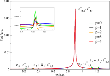
Figure 1: Modulus of the discrete Fourier transform of the current for $V_{g}=-1.4$ a.u. and a constant bias in the left lead $U_{L}=0.1$ a.u.. The inset shows a magnification of the region with bound-continuum transitions from the bound state with higher energy to the Fermi energy. Different curves correspond to different time intervals.

The biased Hamiltonian has two bound eigenstates with energies $\varepsilon_{b,1}^{\infty}=-1.032$ a.u. and $\varepsilon_{b,2}^{\infty}=-0.133$ a.u.. From the discussion of the previous Section we expect that a steady state cannot develop and that the time-dependent current exhibits an oscillatory behavior with frequency $\omega_{0}=\varepsilon_{b,2}^{\infty}-\varepsilon_{b,1}^{\infty}$. This is indeed confirmed by our numerical simulations, as one can see in Fig. 1 where we plot the modulus of the discrete Fourier transform of the time-dependent current. The latter quantity is defined according to

$$I(\omega_{k})=\frac{2\delta}{\pi\sqrt{2N_{0}}}\sum_{n=n_{p}}^{n_{p}+N_{0}}I(2n\delta)e^{-i\omega_{k}n\delta},\quad\omega_{k}=\frac{2\pi k}{N_{0}\delta}.$$ (23)

We have computed ${I}(\omega_{k})$ for different values of $n_{p}=(4+2p)\cdot 10^{3}$, $p=0,1,2,3,4$, and $N_{0}=16\cdot 10^{3}$. Different values of $p$ correspond to different time intervals $t\in(t_{p},t_{p}+T_{0})$ with $t_{p}=(2+p)\times 100$ a.u. but with the same duration $T_{0}=800$ a.u.. The coefficient in Eq. (23) is defined such that the height of the peak $I(\omega)$ at $\omega$ is equal to the amplitude of the oscillations with frequency $\omega$. Besides the zero-frequency peak (not shown) due to the non vanishing dc current, ${I}(\omega)$ shows a dominant peak at the frequency $\omega_{0}=\varepsilon_{b,2}^{\infty}-\varepsilon_{b,1}^{\infty}$ of the transition between the two bound states. As expected, the height of this peak remains unchanged as $p$ varies from 0 to 4, i.e., the current oscillation associated with this transition remains undamped. We emphasize that they are an intrinsic property of the biased system.

Closer examination of Fig. 1 reveals four extra peaks which are related to different internal transitions. The first and the last pairs of peaks occur at frequencies which correspond to transitions between the bound states and the lower edge of the unoccupied part of the continuous spectrum in the left and right lead of the biased system, $\varepsilon_{b,i}^{\infty}\rightarrow\varepsilon_{\rm F}$, and $\varepsilon_{b,i}^{\infty}\rightarrow\varepsilon_{\rm F}+U_{L}$, with $i=1,2$. These sharp structures (mathematically stemming from the discontinuity of the zero-temperature Fermi distribution function) give rise to long-lived oscillations of the total current and density. These oscillatory transients die off very slowly, the height of the peaks decreases with increasing $t_{p}$ empirically as $1/t_{p}$ (power-law behavior).

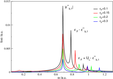
Figure 2: Modulus of the discrete Fourier transform of the current of a translationally invariant initial Hamiltonian which is perturbed at $t=0$ by a sudden bias in the left lead $U_{L}=0.15$ a.u. and the system evolves toward a steady state. Then, at $T=150$ a.u. a gate voltage $V_{g}(x)=-v_{g}=-1.02$ a.u. is suddenly turned on. The first peak appears at the $\omega=0.686$ a.u. which is the modulus of the energy of the bound eigenstate of the final Hamiltonian ($H(x,t>T)$ has one bound eigenstate). Different curves correspond to different Fermi energies.

In Fig. 1, as well as in all following examples, we report results for the current calculated in the center of the device region. However it is worth to mention that the amplitude of the current oscillations decays exponentially in the leads as $e^{-(k^{\alpha}_{b,1}+k^{\alpha}_{b,2})|x-x_{\alpha}|}~{}$ where $k^{\alpha}_{b,i}=\sqrt{2(|\varepsilon_{b,i}^{\infty}|+U_{\alpha})}$ with $i=1,2$, $\alpha=L,R$ and $x$ is a point in lead $\alpha$. Consequently, the dynamical part of the current vanishes deep inside the leads (away from where the bound states are localized).

In the second example, we consider a system described by the translationally invariant Hamiltonian $H(x,t<0)=-\frac{1}{2}\frac{{\rm d}^{2}}{{\rm d}x^{2}}$. At $t=0$ we suddenly switch on a constant bias in the left lead $U_{L}=0.15$ a.u. and propagate until $T=150$ a.u. when a steady state is reached. At $t=T$ a gate voltage $V_{g}(x)=-v_{g}=-1.02$ a.u. is suddenly turned on and the Hamiltonian $H(x,t>T)$ has one bound eigenstate at energy $\varepsilon^{\infty}_{b}=-0.686$ a.u. . The depth $v_{g}$ is chosen in such a way that if one slightly increases $v_{g}$ a second bound eigenstate appears. Since the system has only one bound state, the oscillations die out slowly as $1/(t-T)$ and eventually another steady state develops. In order to understand the transient oscillations we have studied the Fourier transform of the current as shown in Fig. 2. There the first peak appears at the frequency of $\omega=|\varepsilon_{b,1}^{\infty}|$ which is a transition between the bound level and the bottom of the continuum. As such, the position of this peak remains unchanged for different Fermi energies. Besides this transition one observes other peaks whose positions shift as the Fermi energy is changed. They correspond to transitions from the bound level to the top of the left and right continua and, as for the first transition, they decay as $1/(t-T)$.

III.2 Dependence of the current oscillations on the initial conditions

The dynamical part of the current depends on the initial Hamiltonian $H^{0}(x)$ through the amplitudes $f_{b,b^{\prime}}$ of Eq. (9). In the first example of the previous Section the Hamiltonian at negative times, $H^{0}(x)$, had no bound eigenstates. At positive times a gate voltage and a bias in the left lead were suddenly switched on and the Hamiltonian at positive times is equal to $H^{\infty}(x)$ and has two bound eigenstates. We now consider a system with two bound eigenstates for $t\leq 0$ and exposed to a dc bias for $t>0$. Specifically, we start with a static potential describing a quantum well of depth $U_{0}(x)=-1.4$ a.u. for $|x|<1.2$ a.u.. The ground state of the system is the Slater determinant of all the extended eigenstates with energy up to $\varepsilon_{\rm F}=0.1$ a.u. and of the two bound eigenstates at energies $\varepsilon^{0}_{b,1}=-1.035$ a.u. and $\varepsilon^{0}_{b,2}=-0.156$ a.u.. At $t=0$ a dc bias $U_{R}=0.1$ a.u. is suddenly switched on in the left lead and the Hamiltonian $H(x,t>0)=H^{\infty}(x)$ is equal to the final Hamiltonian studied in the previous Section. The resulting time-dependent current for these two systems are shown in Fig. 3.

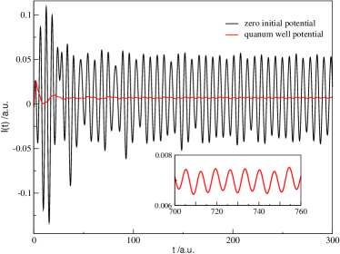
Figure 3: Comparison of the time-dependent current for systems with and without bound states at negative times. The inset shows a magnification of the time-dependent current of the system with two initial bound states. Since both systems have the same final Hamiltonian, the frequencies of the current oscillations are the same while the amplitude of the oscillations for the quantum well (with two bound state initially) is smaller by almost two orders of magnitude than for the system without initial bound states.

As a consequence of the fact that $H^{\infty}(x)$ is the same in both systems the time-dependent currents should oscillate with the same frequency, a result which is confirmed by our numerical calculation. The amplitude of this oscillation, however, depends on the initial equilibrium configuration as well as on how $H(x,t)$ approaches the asymptotic Hamiltonian $H^{\infty}(x)$. As one can see from Fig. 3, the amplitude is much larger in the system with no initial bound states. This difference can be explained qualitatively by looking at Eq. (9). In both systems the time-dependent perturbation is switched on suddenly. Therefore, the transformation matrix of Eq. (10) becomes the unit matrix and Eq. (9) reduces to

$$f_{b,b^{\prime}}=\langle\psi^{\infty}_{b}|f(\mbox{\boldmath$H$}^{0})|\psi^{\infty}_{b^{\prime}}\rangle.$$ (24)

When the perturbation is small like in the case of the system with two initial bound states ($\mbox{\boldmath$H$}^{0}\approx\mbox{\boldmath$H$}^{\infty}$), the eigenfunctions $|\psi_{b}^{\infty}\rangle$ of $\mbox{\boldmath$H$}^{\infty}$ are approximate eigenfunctions of $\mbox{\boldmath$H$}^{0}$ as well. Therefore $f(\mbox{\boldmath$H$}^{0})|\psi_{b}^{\infty}\rangle\approx f(\varepsilon_{b})|\psi_{b}^{\infty}\rangle$ and $f_{b,b^{\prime}}\approx f(\varepsilon_{b})\delta_{b,b^{\prime}}$ which leads to a vanishing dynamical part of the current since there only the off-diagonal elements contribute. By contrast, if the applied potential $U(x,t)$ is large, the overlap $\langle\psi^{\infty}_{b}|f(\mbox{\boldmath$H$}^{0})|\psi^{\infty}_{b^{\prime}}\rangle$ can be quite substantial and the resulting amplitude of the current oscillation is large.

III.3 Dependence of the current oscillations on the history of the bias

The amplitude of the bound state oscillations depends, through the transformation matrix in Eq. (10), on the history of the time-dependent potential which perturbs the initial state. In this Section we investigate for the first time how such amplitudes depend on the switching process (history-dependence effects).

We take the flat potential $U_{0}(x)=0$ as initial potential and the Fermi energy $\epsilon_{\rm F}=0.2$ a.u.. At $t=0$ a gate voltage $V_{g}(x)=-1.3$ a.u. abruptly lowers the potential in the center. In addition, a time-dependent bias is applied to the left lead as $U_{L}(t)=U_{L}\sin^{2}(\omega_{b}t)$ for $t\leq t_{b}=\frac{\pi}{2\omega_{b}}$ and $U_{L}(t)=U_{L}$ for $t>\frac{\pi}{2\omega_{b}}$, where $U_{L}=0.1$ a.u..

The final biased Hamiltonian has two bound states with energies $\epsilon_{b,1}^{\infty}=-0.933$ a.u. and $\epsilon_{b,2}^{\infty}=-0.063$ a.u. which again leads to undamped oscillations in the current.

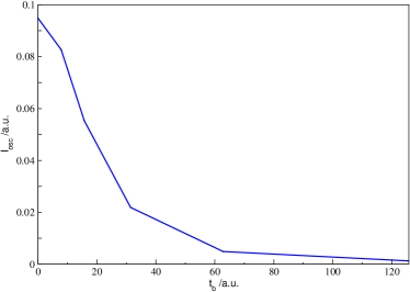
Figure 4: The amplitude of the current oscillation as function of the switching time of the bias. The bias in the left lead is switched according to $U_{L}(t)=U_{L}\sin^{2}(\omega_{b}t)$ for $t\leq t_{b}=\frac{\pi}{2\omega_{b}}$ and $U_{L}(t)=U_{L}=0.1$ a.u. for later times. The frequency of the current oscillation $\omega_{0}=\epsilon_{b,2}^{\infty}-\epsilon_{b,1}^{\infty}$ is given by the difference of bound state energies in the final system which have the values $\epsilon_{b,1}^{\infty}=-0.933$ a.u. and $\epsilon_{b,2}^{\infty}=-0.063$ a.u., respectively. The Fermi energy is $\epsilon_{\rm F}=0.2$ a.u. and the gate potential is $V_{g}=-1.3$ a.u..

Choosing $t_{b}$ in such a way that $\Delta^{\infty}_{L}$ equals $2\pi$, $4\pi$,…the upper block of the unitary matrix in Eq. (10) become the identity matrix in region $L$. This suggests that the amplitude of the current oscillations might exhibit a non-monotonic behavior as a function of the switching time. Our numerical results demonstrate that this is not the case. Fig. 4 shows that the amplitude decreases monotonically as a function of $t_{b}$, a trend which is expected in the region of long switching times (adiabatic switching). Such behavior, however, does not contradict the analytic results of Section II.1. In fact, the memory matrix in the central region $\mbox{\boldmath$M$}_{C}$ also depends on the way the bias is switched on through the time-dependent embedding self-energy needed to calculate $\mbox{\boldmath$G$}^{A}_{CC}(0;t)$, see Eq. (12), and, in general, $\mbox{\boldmath$M$}_{C}\neq{\mbox{\boldmath$1$}}_{C}$ when $\Delta_{L}^{\infty}=2\pi,\;4\pi,\ldots$

III.4 Dependence of the current oscillations on the history of the gate voltage

Finally we present some results to illustrate the dependence of the current oscillations on the switching process of the gate voltage.

Figure 5: Schematic sketch of the time evolution of the Hamiltonian. Starting from an initially constant potential (left), at $t=0$ a bias is suddenly applied to the left lead and the system evolves toward a steady state (center). Then, between times $T$ and $T+t_{g}$, a time-dependent gate voltage $V_{g}(x,t)=-\frac{v_{g}}{t_{g}}(t-T)$ is switched on in region $C$. For times $t>T+t_{g}$ (right) the Hamiltonian remains constant in time.

Again we start with the constant potential $U_{0}(x)=0$ at equilibrium. At $t=0$ a bias is ramped up abruptly in the left lead and the time-dependent current goes through some transient which lasts for a few tens of atomic units. We wait long enough, a time $T=150$ a.u., for a steady-state to develop. After this time all dependence on the history of the applied bias is washed out.

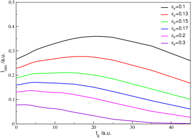
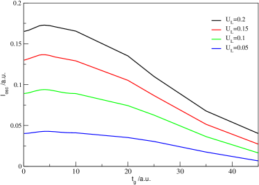
Figure 6: The amplitude of the current oscillations as function of the switching time $t_{g}$ for $v_{g}=1.3$ a.u.. Upper panel: for fixed bias $U_{L}=0.15$ a.u. and different Fermi energies. Lower panel: for fixed Fermi energy $\varepsilon_{\rm F}=0.2$ a.u. and different values of the bias. All curves reach a maximum whose position remains almost unchanged.

At $t=T$ a time dependent gate voltage $V_{g}(x,t)=-\frac{v_{g}}{t_{g}}(t-T)$ is applied to region $C$. The gate voltage decreases linearly until $t=T+t_{g}$ and remains constant and equal to $-v_{g}$ for all later times. In Fig. 5 we provide a schematic sketch of the overall time-dependent perturbation.

The time $t_{g}$ is the switching time. The final Hamiltonian $H^{\infty}(x)=H(x,t>T+t_{g})$ has two bound eigenfunctions and the steady-state cannot develop.

In Fig. 6 the amplitude of the oscillation versus the switching time $t_{g}$ is shown for a final depth of the gate $v_{g}=1.3$ a.u.. In the upper panel, the bias in the left lead is fixed to $U_{L}=0.15$ a.u. and the Fermi energy is varied from $\varepsilon_{\rm F}=0.1$ a.u. to $0.3$ a.u.. We see that the amplitude reaches a maximum value for a certain switching time. It is also worth noting that the amplitudes are generally smaller for larger Fermi energies, a behavior which can be explained as follows: let $|\phi_{n}\rangle$ be an eigenstate of $\mbox{\boldmath$H$}^{0}$ with eigenenergy $\varepsilon_{n}$. Then

$$f_{b,b^{\prime}}=\sum_{\varepsilon_{n}<\varepsilon_{\rm F}}\langle\psi^{\prime}_{b}|\phi_{n}\rangle\langle\phi_{n}|\psi^{\prime}_{b^{\prime}}\rangle.$$ (25)

As the Fermi energy increase the sum over $\varepsilon_{n}$ approaches the sum over a complete set of eigenstates and hence $f_{b,b^{\prime}}$ approaches the value $\langle\psi^{\prime}_{b}|\psi^{\prime}_{b^{\prime}}\rangle$. This latter quantity vanishes since the states $|\psi^{\prime}_{b}\rangle$ are related to the orthogonal states $|\psi^{\infty}_{b}\rangle$ by a unitary transformation and hence remain orthogonal. The lower panel of Fig. 6 shows the amplitude versus the switching time of the gate voltage for a fixed Fermi energy $\varepsilon_{\rm F}=0.2$ a.u. and for different values of the applied bias. The striking feature of this plot is that the position of the maximum remains almost unchanged as function of the bias $U_{L}$.

As a final example, in Fig. 7 we compare the amplitude of the oscillations as function of the switching time $t_{g}$ for two different initial states with the same Fermi energy $\varepsilon_{\rm F}=0.1$ a.u. In one case we start, as before, with the constant potential $U_{0}(x)=0$, and hence $H^{0}(x)$ does not have bound eigenstates. In the other case we start with a quantum well of depth $U_{0}=-0.5$ a.u. for $|x|\leq 1.2$ a.u.. The Hamiltonian $H^{0}(x)$ in this latter case has one bound eigenstate. A bias $U_{L}=0.15$ a.u. in the left lead is suddenly switched on in both systems and after a time $T=150$ a.u. a steady state is attained. For $T<t<T+t_{g}$ a gate voltage $V_{g}(x,t)$ is gradually switched on as before, and for $t>T+t_{g}$ the gate voltage remains constant and equal to $v_{g}=-1.3$ a.u. in the first case and $-0.8$ a.u. in the second case. Hence, both systems have the same asymptotic Hamiltonian $H^{\infty}(x)$. The remarkable difference between the value of the amplitudes in these cases can be explained in the same way as in Section III.2.

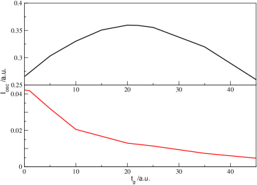
Figure 7: The amplitude of the current oscillation as function of the switching time of the gate. The red (black) curve refers to the initial ground state with (without) a bound state. The numerical parameters are $\varepsilon_{\rm F}=0.1$ a.u., $U_{L}=0.15$ a.u.

Interestingly, in the case where the system initially has one bound state, the amplitude has a maximum for sudden switching of the gate, i.e., $t_{g}=0$ a.u., while in the case with no initial bound states the maximum appears at a finite value of $t_{g}$.

Similarly, we have found a maximum for small $t_{g}$ for the following situation: we start with an initial state without bound states. At $t=0$ a.u. we suddenly apply a bias in the left lead and wait until a steady state is achieved. Then we switch on a gate in such a way that one bound state is created and wait until the associated bound-continuum transitions have decayed before we add another bound state to the gate with a switching time $t_{g}$.

The fact that in this case the largest amplitude for the current oscillations is found for switching time $t_{g}$ close to zero strongly suggests that the position of the maximum in the oscillation amplitude as function of $t_{g}$ is related to a transient effect. This is also supported by the following observation (see Fig.6): the switching time $t_{g}$ for which the current oscillations are largest depends on the Fermi energy (for fixed bias) since the transitions from the bound states to the top of the Fermi sea obviously depend on $\varepsilon_{\rm F}$. At the same time, the position of this maximum is almost independent of the bias (for fixed Fermi energy) since the bias only leads to a slight energy shift for the bound states.

IV Conclusions

In the theory of electron transport one usually assumes that the application of a dc bias to an electronic system attached to two macroscopic electrodes always leads to the evolution of a steady-state current. Recent theoretical work states Stefanucci (2007) that the presence of bound states leads to qualitatively new features (current oscillations and memory effects) in the dynamics of electron transport in the long-time limit. These as well as transient features are investigated here in detail by numerical simulations. In the Fourier transform of the calculated time-dependent current one not only finds the predicted transitions between the bound states in the long-time limit, but, moreover, transitions (in the transient regime) between the bound states and the continuum of the leads can also be clearly identified. We have shown that the amplitude of the persistent current oscillations depends both on the initial state and on the history of system. Since current and density are related via the continuity equation, also the time-dependent density in the long-time limit will therefore be history-dependent. Interestingly, these memory effects show up not only in the dynamical part but also in the time-independent contribution of the bound states to the density Khosravi et al. .

Our results indicate that in transport calculations special care has to be taken if bound states are present in the biased system. A warning flag has already to be raised at the assumption of the evolution to a steady state which is not true in general. Of course, the theoretical analysis predicts the existence of oscillations in the current but makes no statement on their relative importance as compared to the steady-state contribution. Our results show, however, that the amplitude of the oscillations locally may very well be comparable or even larger than the steady-state current and therefore cannot be neglected. We would also like to point out that the existence of bound states in biased transport systems may not be an exotic feature in an experimental situation. For single molecules attached to metallic leads it is quite conceivable that some of the molecular orbitals energetically fall into an energy window which corresponds to an energy gap of the leads and those orbitals therefore cannot hybridize with any lead states and remain fully localized. In the case of transport experiments on quantum dots one could artificially create bound states by applying a strong attractive gate potential.

Although our numerical simulations were performed for non-interacting electrons, the conclusions about the dynamical current oscillations apply to any effective single-electron theory. In particular they also apply to the TD Kohn-Sham equations which are in principle able to reproduce the time-dependent densityRunge and E.K.U. Gross (1984) (and the longitudinal current via the continuity equation) of an interacting system if the exact exchange-correlation functional is used. Intuitively, one might expect that electron-electron scattering leads to a damping of the oscillations in the long-time limit. However, the assumption of a time-independent density producing a static Kohn-Sham potential for large times leads to a contradiction if this potential supports bound states since the density and therefore also the Kohn-Sham potential should then become time-dependent again.

References

- Landauer (1957) R. Landauer, IBM J. Res. Develop. 1, 233 (1957).
- Büttiker (1986) M. Büttiker, Phys. Rev. Lett. 57, 1761 (1986).
- M.A. Reed et al. (1997) M.A. Reed, C. Zhou, C.J. Muller, T.P. Burgin, and J.M. Tour, Science 278, 252 (1997).
- N.D. Lang (1995) N.D. Lang, Phys. Rev. B 52, 5335 (1995).
- Hirose and Tsukada (1995) K. Hirose and M. Tsukada, Phys. Rev. B 51, 5278 (1995).
- J.M. Seminario et al. (1998) J.M. Seminario, A.G. Zacarias, and J.M. Tour, J. Am. Chem. Soc. 120, 3970 (1998).
- Taylor et al. (2001) J. Taylor, H. Guo, and J. Wang, Phys. Rev. B 63, 245407 (2001).
- Palacios et al. (2001) J. J. Palacios, A. J. Pérez-Jiménez, E. Louis, and J. Vergés, Phys. Rev. B 64, 115411 (2001).
- Xue et al. (2002) Y. Xue, S. Datta, and M.A. Ratner, Chem. Phys. 281, 151 (2002).
- Brandbyge et al. (2002) M. Brandbyge, J.-L. Mozos, P. Ordejón, J. Taylor, and K. Stokbro, Phys. Rev. B 65, 165401 (2002).
- Evers et al. (2004) F. Evers, F. Weigend, and M. Koentopp, Phys. Rev. B 69, 235411 (2004).
- Faleev et al. (2005) S. V. Faleev, F. Leonard, D. A. Stewart, and M. van Schilfgaarde, Phys. Rev. B 71, 195422 (2005).
- Koentopp et al. (2008) M. Koentopp, C. Chang, K. Burke, and R. Car, J. Phys. Condens. Matter 20, 083203 (2008).
- Kurth et al. (2005) S. Kurth, G. Stefanucci, C.-O. Almbladh, A. Rubio, and E.K.U. Gross, Phys. Rev. B 72, 035308 (2005).
- Bushong et al. (2005) N. Bushong, N. Sai, and M. D. Ventra, Nano Lett. 5, 2569 (2005).
- Sanchez et al. (2006) C. G. Sanchez, M. Stamenova, S. Sanvito, D. R. Bowler, A. P. Horsfield, and T. N. Todorov, J. Chem. Phys. 124, 214708 (2006).
- Sai et al. (2007) N. Sai, N. Bushong, R. Hatcher, and M. D. Ventra, Phys. Rev. B 75, 115410 (2007).
- Cini (1980) M. Cini, Phys. Rev. B 22, 5887 (1980).
- Stefanucci and C.-O. Almbladh (2004a) G. Stefanucci and C.-O. Almbladh, Phys. Rev. B 69, 195318 (2004a).
- Dhar and Sen (2006) A. Dhar and D. Sen, Phys. Rev. B 73, 085119 (2006).
- Stefanucci (2007) G. Stefanucci, Phys. Rev. B 75, 195115 (2007).
- Moldoveanu et al. (2007) V. Moldoveanu, V. Gudmundsson, and A. Manolescu, Phys. Rev. B 76, 165308 (2007).
- Blandin et al. (1976) A. Blandin, A. Nourtier, and D. W. Hone, J. Phys. (Paris) 37, 369 (1976).
- Danielewicz (1984) P. Danielewicz, Ann. Phys. (N. Y.) 152, 239 (1984).
- Stefanucci and C.-O. Almbladh (2004b) G. Stefanucci and C.-O. Almbladh, Europhys. Lett. 67, 14 (2004b).
- Runge and E.K.U. Gross (1984) E. Runge and E.K.U. Gross, Phys. Rev. Lett. 52, 997 (1984).
- E.K.U. Gross and Kohn (1990) E.K.U. Gross and W. Kohn, Adv. Quantum Chem. 21, 255 (1990).
- Verdozzi et al. (2006) C. Verdozzi, G. Stefanucci, and C.-O. Almbladh, Phys. Rev. Lett. 97, 046603 (2006).
- Zhu et al. (2005) Y. Zhu, J. Maciejko, T. Ji, H. Guo, and J. Wang, Phys. Rev. B 71, 075317 (2005).
- Maciejko et al. (2006) J. Maciejko, J. Wang, and H. Guo, Phys. Rev. B 74, 085324 (2006).
- L.P. Kadanoff and Baym (1962) L.P. Kadanoff and G. Baym, Quantum Statistical Mechanics (Benjamin, New York, 1962).
- N.E. Dahlen and R. van Leeuwen (2007) N.E. Dahlen and R. van Leeuwen, Phys. Rev. Lett. 98, 153004 (2007).
- (33) G. Stefanucci, S. Kurth, A. Rubio, and E.K.U. Gross, Phys. Rev. B (in press) and cond-mat/0701209 (2007).
- (34) E. Khosravi, G. Stefanucci, S. Kurth, and E.K.U. Gross, in preparation.