Oscillations of Mössbauer neutrinos

Abstract

We calculate the probability of recoilless emission and detection of neutrinos (Mössbauer effect with neutrinos) taking into account the boundedness of the parent and daughter nuclei in the neutrino source and detector as well as the leptonic mixing. We show that, in spite of their near monochromaticity, the recoillessly emitted and captured neutrinos oscillate. After a qualitative discussion of this issue, we corroborate and extend our results by computing the combined rate of $\bar{\nu}_{e}$ production, propagation and detection in the framework of quantum field theory, starting from first principles. This allows us to avoid making any a priori assumptions about the energy and momentum of the intermediate-state neutrino. Our calculation permits quantitative predictions of the transition rate in future experiments, and shows that the decoherence and delocalization factors, which could in principle suppress neutrino oscillations, are irrelevant under realistic experimental conditions.

I Introduction

Soon after the discovery of recoil-free emission and absorption of gamma rays by Mössbauer in 1958 Mössbauer (1958); Frauenfelder (1962), it has been suggested by Visscher that a similar effect should also exist for neutrinos emitted in electron capture processes from unstable nuclei embedded into a crystal lattice Visscher (1959). In the 1980’s, the idea was further developed by Kells and Schiffer Kells (1983); Kells and Schiffer (1983), who showed that bound state beta decay Bahcall (1961) could provide an alternative recoilless production mechanism. In this case, an antineutrino with a very small energy uncertainty would be emitted, which could then be absorbed through induced orbital electron capture Mikaelyan et al. (1967). Recently, there has been a renewed interest in this idea, inspired by two works by Raghavan Raghavan (2005, 2006), in which the feasibility of an experiment using the emission process

$${}^{3}{\rm H}\ \rightarrow\ {}^{3}{\rm He}\leavevmode\nobreak\ +\leavevmode\nobreak\ e^{-}\text{(bound)}\leavevmode\nobreak\ +\leavevmode\nobreak\ \bar{\nu}_{e}$$ (1)

and the detection process

$${}^{3}{\rm He}\leavevmode\nobreak\ +\leavevmode\nobreak\ e^{-}\text{(bound)}\leavevmode\nobreak\ +\leavevmode\nobreak\ \bar{\nu}_{e}\ \ \rightarrow\ ^{3}{\rm H}$$ (2)

has been studied. The ${}^{3}{\rm H}$ and ${}^{3}{\rm He}$ atoms were proposed to be embedded into metal crystals. The detection process would then have a resonance nature, leading to an enhancement of the detection cross section by up to a factor of $10^{12}$ compared to the non-resonance capture of neutrinos of the same energy. If such an experiment were realized, it could carry out a very interesting physics program, including neutrino detection with 100 g scale (rather than ton or kiloton scale) detectors, searching for neutrino oscillations driven by the mixing angle $\theta_{13}$ at a baseline of only 10 m, determining the neutrino mass hierarchy without using matter effects, searching for active-sterile neutrino oscillations and studying the gravitational redshift of neutrinos Raghavan (2005, 2006); Minakata and Uchinami (2006); Minakata et al. (2007).

In this paper we consider recoillessly emitted and captured neutrinos – which we will call Mössbauer neutrinos – from a theoretical point of view. In our discussion, we will mainly focus on the ${}^{3}{\rm H}$ –${}^{3}{\rm He}$ system of Eqs. (1) and (2), but most of our results apply also to other emitters and absorbers of Mössbauer neutrinos.

One of our main goals is to resolve the recent controversy about the question of whether Mössbauer neutrinos would oscillate. It has been argued Bilenky et al. (2007) that the answer to this question depends on whether equal energies or equal momenta are assumed for different neutrino mass eigenstates – the assumptions often made in deriving the standard formula for the oscillation probability. Moreover, a possible inhibition of oscillations due to the time-energy uncertainty relation has been brought up Bilenky (2007). To come to definitive conclusions regarding the oscillation phenomenology of Mössbauer neutrinos, we employ a quantum field theoretical (QFT) approach, in which neutrinos are treated as intermediate states in the combined production – propagation – detection process and no a priori assumptions on the energies or momenta of the different neutrino mass eigenstates are made.

We begin in Sec. II by qualitatively discussing how the peculiar features of Mössbauer neutrinos, and in particular their very small energy uncertainty, affect the oscillation phenomenology. We argue that oscillations do occur, and that the coherence length is infinite if line broadening is neglected. We then proceed to quantitative arguments in Sec. III and discuss a formula for the $\bar{\nu}_{e}$ survival probability in the quantum mechanical intermediate wave packet formalism Giunti and Kim (1998), in which the neutrino is described as a superposition of three wave packets, one for each mass eigenstate. In Sec. IV, we derive our main result, the rate for the combined process of neutrino production, propagation and detection in the QFT external wave packet approach. In this framework, the neutrino is described by an internal line in a Feynman diagram, while its production and detection partners are described by wave packets. Also in this section, for the first time, we calculate the rates for beta decay with production of a bound-state electron and for the inverse process of stimulated electron capture in the case of nuclei bound to a crystal lattice. We distinguish between different neutrino line broadening mechanisms and concentrate on the oscillation phenomenology, paying special attention to the coherence and localization terms in the $\bar{\nu}_{e}$ survival probability and to the Mössbauer resonance conditions arising in each case. In Sec. V, we discuss the obtained results and draw our conclusions.

II Mössbauer neutrinos do oscillate

Mössbauer neutrinos have very special properties compared to those of neutrinos emitted and detected in conventional processes. In particular, they are almost monochromatic because they are produced in two-body decays of nuclei embedded in a crystal lattice and no phonon excitations of the host crystal accompany their production, which ensures the recoilless nature of this process. Therefore the width of the neutrino line is only limited by the natural linewidth, which is the reciprocal of the mean lifetime of the emitter, and by solid-state effects, including electromagnetic interactions of the randomly oriented nuclear spins, lattice defects and impurities Raghavan (2006); Potzel (2006); Coussement et al. (1992a); Balko et al. (1997). For ${}^{3}{\rm H}$ decay, the natural linewidth is $1.17\cdot 10^{-24}$ eV, but it has been estimated that various broadening effects degrade this value to an experimentally achievable Mössbauer linewidth of $\gamma=\mathcal{O}(10^{-11}\ \text{eV})$ Potzel (2006); Coussement et al. (1992a). Compared to the neutrino energy in bound state ${}^{3}{\rm H}$ decay, $E=18.6$ keV, the achievable relative linewidth is therefore of order $10^{-15}$.

In the standard derivations of the neutrino oscillation formula it is often assumed that the different neutrino mass eigenstates composing the produced flavor eigenstate have the same momentum ($\Delta p=0$), while their kinetic energies differ by $\Delta E\simeq\Delta m^{2}/2E$. For bound state tritium beta decay (1) and $\Delta m^{2}=\Delta m_{31}^{2}\simeq 2.5\times 10^{-3}$ eV² one has $\Delta E\simeq 7\times 10^{-8}$ eV, which is much larger than $\gamma$. One may therefore wonder if the extremely small energy uncertainty of Mössbauer neutrinos would inhibit oscillations by destroying the coherence of the different mass eigenstates of which the produced $\bar{\nu}_{e}$ is composed. Indeed, if neutrinos are emitted with no momentum uncertainty and their energy uncertainty ($\sim\gamma$) is much smaller than the energy differences of the different mass eigenstates, in each decay event one would exactly know which mass eigenstate has been emitted. This would prevent a coherent emission of different mass eigenstates, thus destroying neutrino oscillations. If, on the contrary, one adopts the same energy assumption, the momenta of different mass eigenstates would differ by $\Delta p\simeq\Delta m^{2}/2p$, which would not destroy their coherence provided that the momentum uncertainty of the emitted neutrino state is greater that $\Delta p$; in that case, oscillations are possible.

It is well known that in reality neither same momentum nor same energy assumptions are correct Winter (1981); Giunti et al. (1991); Giunti and Kim (2001); Giunti (2001, 2004); however, for neutrinos from conventional sources both lead to the correct result, the reason being that neutrinos are ultra-relativistic and the spatial size of the corresponding wave packets is small compared to the oscillation length. The above assumptions are thus just shortcuts which allow one to arrive at the correct result in an easy (though not rigorous) way. However, Mössbauer neutrinos represent a very peculiar case, which requires a special consideration.

Let us discuss the issue of coherence of different mass eigenstates in more detail. If one knows the values of the neutrino energy $E$ and momentum $p$ with uncertainties $\sigma_{E}$ and $\sigma_{p}$, from the energy-momentum relation of relativistic particles $E^{2}=p^{2}+m^{2}$ one can infer the value of the squared neutrino mass $m^{2}$ with the uncertainty

$$\sigma_{m^{2}}=\sqrt{(2E\sigma_{E})^{2}+(2p\sigma_{p})^{2}}\,,$$ (3)

where it is assumed that $\sigma_{E}$ and $\sigma_{p}$ are independent. By $\sigma_{E}$ and $\sigma_{p}$ we will now understand the intrinsic quantum mechanical uncertainties of the neutrino energy and momentum, beyond which these quantities cannot be measured in a given production or detection process; $\sigma_{m^{2}}$ is then the quantum mechanical uncertainty of the inferred neutrino squared mass. A generic requirement for coherent emission of different mass eigenstates is their indistinguishability: the uncertainty $\sigma_{m^{2}}$ has to be larger than the mass squared difference $\Delta m^{2}$  Kayser (1981). From the above discussion, we know that for Mössbauer neutrinos corresponding to the ${}^{3}{\rm H}$ –${}^{3}{\rm He}$ system one has $E\sigma_{E}\sim 10^{-8}$ eV², which is much smaller than $\Delta m^{2}\sim 10^{-3}$ eV². Thus, whether or not Mössbauer neutrinos oscillate depends on whether or not $2p\sigma_{p}>\Delta m^{2}$.

While the energy of Mössbauer neutrinos is very precisely given by the production process itself, this is not the case for their momentum. The neutrino momentum can in principle be determined by measuring the recoil momentum of the crystal in which the emitter is embedded. The ultimate uncertainty $\sigma_{p}$ of this measurement is related to the coordinate uncertainty $\sigma_{x}$ of the emitting nucleus through the Heisenberg relation $\sigma_{p}\sigma_{x}\geq 1/2$. Therefore, for the momentum uncertainty to be small enough to destroy the coherence of different mass eigenstates, $2p\sigma_{p}<\Delta m^{2}$, the coordinate uncertainty of the emitter must satisfy $\sigma_{x}\gtrsim 2p/\Delta m^{2}$. This means that the emitter should be strongly de-localized with the coordinate uncertainty $\sigma_{x}$ of order of the neutrino oscillation length $L^{\rm osc}=4\pi p/\Delta m^{2}\simeq 20$ m. This is certainly not the case, because the coordinate uncertainty of the emitter cannot exceed the size of the source, i.e. a few cm. In fact, it is even much smaller, because in principle it is possible to find out which particular nucleus has undergone the Mössbauer transition by destroying the crystal and checking which ³H atom has been transformed into ³He. Thus, $\sigma_{x}$ is of the order of interatomic distances, i.e. $\sigma_{p}\sim 10$ keV, so that

$$2p\sigma_{p}\gg\Delta m^{2}\,.$$ (4)

This means that Mössbauer neutrinos will oscillate. The condition (4) is often called the localization condition, because it requires the neutrino source to be localized in a spatial region that is small compared to the neutrino oscillation length $L^{\rm osc}$.

It should be noted that for the observability of neutrino oscillations the coherence of the emitted neutrino state is not by itself sufficient; in addition, this state must not lose its coherence until the neutrino is detected. A coherence loss could occur because of the wave packet separation. When a neutrino is produced as a flavour eigenstate, the wave packets of its mass eigenstate components fully overlap; however, since they propagate with different group velocities, after a time $t^{\rm coh}$ or upon propagating a distance $L^{\rm coh}\simeq t^{\rm coh}$, these wave packets separate to such an extent that they can no longer interfere in the detector, and oscillations become unobservable. The coherence length $L^{\rm coh}$ depends on the energy uncertainty $\sigma_{E}$ of the emitted neutrino state and becomes infinite in the limit $\sigma_{E}\to 0$.

From the above discussion it follows that the oscillation phenomenology of Mössbauer neutrinos should mainly depend on their momentum uncertainty, whereas their energy uncertainty, though crucial for the Mössbauer resonance condition, plays a relatively minor role for neutrino oscillations. Therefore, the equal energy assumption, though in general incorrect, should be a good approximation when discussing oscillations of Mössbauer neutrinos. Adopting this approach, i.e. assuming the neutrino energy to be exactly fixed at a value $E$ by the production process, one obtains for the $\bar{\nu}_{e}$ survival probability $P_{ee}$ at a distance $L$

$$P_{ee} =\sum_{j,k}|U_{ej}|^{2}|U_{ek}|^{2}\exp\Big{[}-2\pi i\frac{L}{L^{\rm osc}_{jk}}\Big{]}.$$ (5)

Here $U$ is the leptonic mixing matrix, $L^{\rm osc}_{jk}$ are the partial oscillation lengths,

$$L^{\rm osc}_{jk} =\frac{4\pi E}{\Delta m_{jk}^{2}}\,,$$ (6)

and the neutrinos are assumed to be ultra-relativistic or nearly mass-degenerate, so that

$$\frac{\Delta m_{jk}^{2}}{2E}\ll E\,.$$ (7)

Eq. (5) is just the standard result for the $\bar{\nu}_{e}$ survival probability. As expected, we do not obtain any decoherence factors if the neutrino energy is exactly fixed. We have also taken into account here that in real experiments the size of the source and detector are much smaller than the smallest of the oscillation lengths $L^{\rm osc}_{jk}$, so that the localization condition (4) is satisfied.

III Mössbauer neutrinos in the intermediate wave packet formalism

Although Eq. (5) shows that neutrino oscillations are not inhibited by the energy constraints implied by the Mössbauer effect, the assumption of an exactly fixed neutrino energy is certainly unrealistic. Therefore, we will now proceed to a more accurate treatment of Mössbauer neutrinos using an intermediate wave packet model Giunti et al. (1991, 1992); Kiers et al. (1996); Giunti and Kim (1998); Giunti (2004). In this approach, the propagating neutrino is described by a superposition of mass eigenstates, each of which is in turn a wave packet with a finite momentum width. With the assumption of Gaussian wave packets, Giunti, Kim and Lee Giunti et al. (1992); Giunti and Kim (1998) obtain the following expression for the $\bar{\nu}_{e}$ survival probability in the approximation of ultra-relativistic neutrinos:

$$P_{ee} =\sum_{j,k}|U_{ej}|^{2}|U_{ek}|^{2}\exp\bigg{[}-2\pi i\frac{L}{L^{\rm osc}_{jk}}-\bigg{(}\frac{L}{L^{\rm coh}_{jk}}\bigg{)}^{2}-2\pi^{2}\xi^{2}\bigg{(}\frac{1}{2\sigma_{p}L^{\rm osc}_{jk}}\bigg{)}^{2}\bigg{]}.$$ (8)

Here

$$L^{\rm coh}_{jk} =\frac{2\sqrt{2}E^{2}}{\sigma_{p}|\Delta m_{jk}^{2}|}$$ (9)

are the partial coherence lengths, $\sigma_{p}$ being the effective momentum uncertainty of the neutrino state, and the oscillation lengths $L^{\rm osc}_{jk}$ are given by Eq. (6). $E$ is the energy that a massless neutrino emitted in the same process would have, and the $\mathcal{O}(1)$ parameter $\xi$ quantifies the deviation of the actual energies of massive neutrinos from this value. Since the energy uncertainty is very small for Mössbauer neutrinos, the mass eigenstates differ in momentum, but hardly in energy, so that $\xi$ should be negligibly small in our case.

One can see that the first term in the exponent of Eq. (8) is the standard oscillation phase. The second term yields a decoherence factor, which describes the suppression of oscillations due to the wave packet separation. For conventional neutrino experiments with non-negligible $\xi$, the third term implements a localization condition by suppressing oscillations if the spatial width $\sigma_{x}=1/2\sigma_{p}$ of the neutrino wave packet is much larger than the oscillation length $L^{\rm osc}_{jk}$ (cf. Eqs. (6) and (4)). However, we have seen that, due to the smallness of $\xi$, the intermediate wave packet formalism predicts this condition to be irrelevant for oscillations of Mössbauer neutrinos.

IV Mössbauer neutrinos in the external wave packet formalism

Figure 1: Feynman diagram for neutrino emission and absorption in the ³H –³He system.

In the derivation of the quantum mechanical result discussed in the previous section, certain assumptions had to be made on the properties of the neutrino wave packets, in particular on the parameters $\sigma_{p}$ and $\xi$. We will now proceed to the discussion of a QFT approach Jacob and Sachs (1961); Sachs (1963); Giunti et al. (1993); Rich (1993); Grimus and Stockinger (1996); Grimus et al. (1999, 2000); Cardall (2000); Beuthe (2003, 2002), in which these quantities will be automatically determined from the properties of the source and the detector.

Our calculation will be based on the Feynman diagram shown in Fig. 1, in which the neutrino is described as an internal line. We take the external particles to be confined by quantum mechanical harmonic oscillator potentials to reflect the fact that they are bound in a crystal lattice. Typical values for the harmonic oscillator frequencies are of the order of the Debye temperature $\Theta_{D}\sim 600\ \mathrm{K}\simeq 0.05$ eV of the respective crystals Raghavan (2006); Potzel (2006). Although this simplistic treatment neglects the detailed structure of the solid state lattice, it is known to correctly reproduce the main features of the conventional Mössbauer effect Lipkin (1973), and since we are interested mainly in the oscillation physics and not in the exact overall process rate, it is sufficient for our purposes. As only recoil-free neutrino emission and absorption are of interest to us, we can neglect thermal excitations and consider the parent and daughter nuclei in the source and detector to be in the ground states of their respective harmonic oscillator potentials.

In Sec. IV.1, we will develop our formalism and derive an expression for the rate of the combined process of Mössbauer neutrino emission, propagation and absorption. In Secs. IV.2 – IV.4 we will then discuss in detail the effects of different line broadening mechanisms.

IV.1 The formalism

Let us denote the harmonic oscillator frequencies for tritium and helium in the source by $\omega_{{\rm H},S}$ and $\omega_{{\rm He},S}$ and those in the detector by $\omega_{{\rm H},D}$, and $\omega_{{\rm He},D}$. In general, these are four different numbers because ${}^{3}{\rm H}$ and ${}^{3}{\rm He}$ have different chemical properties, and because their different abundances in the source and detector imply $\omega_{{\rm H},S}\neq\omega_{{\rm H},D}$ and $\omega_{{\rm He},S}\neq\omega_{{\rm He},D}$. We ignore possible anisotropies of the oscillator frequencies because their inclusion would merely lengthen our formulas without giving new insights into the oscillation phenomenology. The normalized wave functions of the ground states of the three-dimensional harmonic oscillators $|\psi_{A,B,0}\rangle$ are given by

$$\psi_{A,B,0}({\mathbf{x}},t)=\bigg{[}\frac{m_{A}\omega_{A,B}}{\pi}\bigg{]}^{\frac{3}{4}}\exp\bigg{[}\!-\frac{1}{2}m_{A}\omega_{A,B}|{\mathbf{x}}-{\mathbf{x}}_{B}|^{2}\bigg{]}\cdot e^{-iE_{A,B}t},$$ (10)

where $A=\{{\rm H},{\rm He}\}$ distinguishes the two types of atoms and $B=\{S,D\}$ distinguishes between quantities related to the source and to the detector. The masses of the tritium and ${}^{3}{\rm He}$ atoms are denoted by $m_{\rm H}$ and $m_{\rm He}$, and the coordinates of the lattice sites at which the atoms are localized in the source and in the detector are ${\mathbf{x}}_{S}$ and ${\mathbf{x}}_{D}$. The energies $E_{A,B}$ of the external particles are not exactly fixed due to the line broadening mechanisms discussed in Sec. II, but follow narrow distribution functions, which are centered around $E_{A,B,0}=m_{A}+\frac{1}{2}\omega_{A,B}$. For the differences of these mean energies of tritium and helium atoms in the source and detector we will use the notation

$$E_{S,0}=E_{{\rm H},S,0}-E_{{\rm He},S,0}\,,\qquad\qquad E_{D,0}=E_{{\rm H},D,0}-E_{{\rm He},D,0}\,.$$ (11)

Before proceeding to calculate the overall rate of the process of neutrino production, propagation and detection, we compute the expected rates of the Mössbauer neutrino production and detection treated as separate processes, ignoring neutrino oscillations. This calculation is very instructive, and we will use its result as a benchmark for comparison with our subsequent QFT calculations.

The effective weak interaction Hamiltonians for the neutrino production and detection $H_{S}^{+}$ and $H_{D}^{-}$ are given by Eqs. (66) and (67) of appendix C. We will first assume that the neutrino emitted in the recoil-free production process (1) is monochromatic, i.e. neglect the natural linewidth as well as all broadening effects. Likewise, we will neglect now the absorption line broadening effects in the recoilless detection process (2). A straightforward calculation gives for the rate of recoilless neutrino production

$$\Gamma_{p}=\Gamma_{0}\,X_{S}\,,$$ (12)

where

$$\Gamma_{0}=\frac{G_{F}^{2}\cos^{2}\theta_{c}}{\pi}\;|\psi_{e}(R)|^{2}\,m_{e}^{2}\,\left(|M_{V}|^{2}+g_{A}^{2}|M_{A}|^{2}\right)\,\left(\frac{E_{S,0}}{m_{e}}\right)^{2}\kappa_{S}$$ (13)

with $G_{F}$ the Fermi constant, $\theta_{c}$ the Cabibbo angle, $m_{e}$ the electron mass, $M_{V}$ and $M_{A}$ the vector and axial-vector (or Fermi and Gamow-Teller) nuclear matrix elements and $g_{A}\simeq 1.25$ the axial-vector coupling constant. Note that for the allowed beta transitions in the ³H –³He system, $M_{V}=1$ and $M_{A}\approx\sqrt{3}$. The quantity $\psi_{e}(R)$ is the value of the anti-symmetrized atomic wave function of ${}^{3}{\rm He}$ at the surface of the nucleus. The factor $\kappa_{S}$ takes into account that the spectator electron which is initially in the $1s$ atomic state of ${}^{3}{\rm H}$ ends up in the $1s$ state of ${}^{3}{\rm He}$. It is given by the overlap integral of the corresponding atomic wave functions:

$$\kappa_{S}\leavevmode\nobreak\ =\leavevmode\nobreak\ \Big{|}\int\Psi_{Z=2,S}({\mathbf{r}})^{*}\,\Psi_{Z=1,S}({\mathbf{r}})\,d^{3}r\,\Big{|}^{2}\,.$$ (14)

The factor $X_{S}$ in Eq. (12) is defined as

$$X_{S}=8\left(\eta_{S}+\frac{1}{\eta_{S}}\right)^{-3}e^{-\frac{p^{2}}{\sigma_{pS}^{2}}}\,\equiv\,Y_{S}\,e^{-\frac{p^{2}}{\sigma_{pS}^{2}}}\,,$$ (15)

where $p=\sqrt{E_{S,0}^{2}-m^{2}}$ is the neutrino momentum, and

$$\eta_{S}=\sqrt{\frac{m_{\rm H}\,\omega_{{\rm H},S}}{m_{\rm He}\,\omega_{{\rm He},S}}}\,,\qquad\qquad\sigma_{pS}^{2}=m_{\rm H}\,\omega_{{\rm H},S}+m_{\rm He}\,\omega_{{\rm He},S}\,.$$ (16)

The energy spectrum $\rho(E)$ of the emitted Mössbauer neutrinos in the considered approximation is

$$\rho(E)=\Gamma_{0}\,X_{S}\,\delta(E-E_{S,0})\,.$$ (17)

For the cross section of the recoilless detection process (2) we obtain

$$\sigma(E)=B_{0}\,X_{D}\,\delta(E-E_{D,0})\,,$$ (18)

where

$$B_{0}=4\pi G_{F}^{2}\cos^{2}\theta_{c}\;|\psi_{e}(R)|^{2}\left(|M_{V}|^{2}+g_{A}^{2}|M_{A}|^{2}\right)\,\kappa_{D}\,.$$ (19)

The factor $\kappa_{D}$ here is defined similarly to $\kappa_{S}$ in Eq. (14). Note that in the approximation of hydrogen-like atomic wave functions one has $\kappa_{S}=\kappa_{D}=512/729\simeq 0.7$. The factor $X_{D}$ in Eq. (18) is defined similarly to the corresponding factor for the production process, i.e.

$$X_{D}=8\left(\eta_{D}+\frac{1}{\eta_{D}}\right)^{-3}e^{-\frac{p^{2}}{\sigma_{pD}^{2}}}\,\equiv\,Y_{D}\,e^{-\frac{p^{2}}{\sigma_{pD}^{2}}}$$ (20)

with

$$\eta_{D}=\sqrt{\frac{m_{\rm H}\,\omega_{{\rm H},D}}{m_{\rm He}\,\omega_{{\rm He},D}}}\,,\qquad\qquad\sigma_{pD}^{2}=m_{\rm H}\,\omega_{{\rm H},D}+m_{\rm He}\,\omega_{{\rm He},D}\,.$$ (21)

The Mössbauer neutrino production rate $\Gamma_{p}$ and detection cross section $\sigma(E)$ differ from those previously obtained for unbound parent and daughter nuclei respectively in Refs. Bahcall (1961) and Mikaelyan et al. (1967) by the factors $X_{S}$ and $X_{D}$. Note that in the limit $m_{\rm H}\,\omega_{{\rm H},S}=m_{\rm He}\,\omega_{{\rm He},S}$, $m_{\rm H}\,\omega_{{\rm H},D}=m_{\rm He}\,\omega_{{\rm He},D}$, the pre-exponential factors $Y_{S}$ and $Y_{D}$ in Eqs. (15) and (20) become equal to unity, so that $X_{S}$ and $X_{D}$ reduce to the exponentials, which are merely the recoil-free fractions in the production and detection processes (see the discussion below).

For unpolarized tritium nuclei in the source the produced neutrino flux is isotropic; therefore the spectral density of the neutrino flux at the detector located at a distance $L$ from the source is $\rho(E)/(4\pi L^{2})$. The detection rate is thus

$$\Gamma\,=\,\frac{1}{4\pi L^{2}}\int_{0}^{\infty}\rho(E)\sigma(E)\,dE\,=\,\frac{\Gamma_{0}\,B_{0}}{4\pi L^{2}}\,X_{S}X_{D}\;\delta(E_{S,0}-E_{D,0})\,.$$ (22)

We see that it is infinite when the Mössbauer resonance condition $E_{S,0}=E_{D,0}$ is exactly satisfied and zero otherwise, which is a consequence of our assumption of infinitely sharp emission and absorption lines. This assumption is certainly unphysical, and a realistic calculation should take into account the finite linewidth effects. We do that here by assuming Lorentzian energy distributions for the production and detection processes, which will be useful for comparison with the results of our subsequent QFT approach. In this approximation Eqs. (17) and (18) have to be replaced by

$$\rho(E)=\Gamma_{0}\,X_{S}\,\frac{\gamma_{S}/2\pi}{(E-E_{S,0})^{2}+\gamma_{S}^{2}/4}\,,\qquad\sigma(E)=B_{0}\,X_{D}\,\frac{\gamma_{D}/2\pi}{(E-E_{D,0})^{2}+\gamma_{D}^{2}/4}\,,$$ (23)

where $\gamma_{S}$ and $\gamma_{D}$ are the energy widths associated with production and detection. The combined rate of the neutrino production, propagation and detection process is then

$$\Gamma\,=\,\frac{1}{4\pi L^{2}}\int_{0}^{\infty}\rho(E)\sigma(E)\,dE\,\simeq\,\frac{\Gamma_{0}\,B_{0}}{4\pi L^{2}}\,X_{S}X_{D}\;\frac{(\gamma_{S}+\gamma_{D})/2\pi}{(E_{S,0}-E_{D,0})^{2}+(\gamma_{S}+\gamma_{D})^{2}/4}\,.$$ (24)

As can be seen from this formula, the Mössbauer resonance condition is

$$(E_{S,0}-E_{D,0})^{2}\ll(\gamma_{S}+\gamma_{D})^{2}/4\,.$$ (25)

If it is satisfied, the neutrino detection cross section is enhanced by a factor of order $(\alpha Zm_{e})^{3}/[p_{e}E_{e}(\gamma_{S}+\gamma_{D})]$ compared to cross sections of non-resonant capture reactions $\bar{\nu}_{e}+A\to A^{\prime}+e^{+}$ for neutrinos of the same energy (assuming the recoil-free fraction to be of order 1). For $\gamma_{S}+\gamma_{D}\sim 10^{-11}$ eV the enhancement factor can be as large as $10^{12}$.

We now turn to the QFT treatment of the overall neutrino production, propagation and detection process, first neglecting the line broadening effects. We derive the corresponding transition amplitude from the matrix elements of the weak currents in the standard way by employing the coordinate-space Feynman rules to the diagram in Fig. 1. For the external tritium and helium nuclei, we use the bound state wave function $\psi_{A,B,0}({\mathbf{x}},t)$ from Eq. (10). We obtain

$$i\mathcal{A} =\int\!d^{3}x_{1}\,dt_{1}\int\!d^{3}x_{2}\,dt_{2}\,\bigg{(}\frac{m_{\rm H}\omega_{{\rm H},S}}{\pi}\bigg{)}^{\frac{3}{4}}\exp\bigg{[}-\frac{1}{2}m_{\rm H}\omega_{{\rm H},S}|{\mathbf{x}}_{1}-{\mathbf{x}}_{S}|^{2}\bigg{]}\,e^{-iE_{{\rm H},S}t_{1}}$$

$$\hskip 28.45274pt\cdot\bigg{(}\frac{m_{\rm He}\omega_{{\rm He},S}}{\pi}\bigg{)}^{\frac{3}{4}}\exp\bigg{[}-\frac{1}{2}m_{\rm He}\omega_{{\rm He},S}|{\mathbf{x}}_{1}-{\mathbf{x}}_{S}|^{2}\bigg{]}\,e^{+iE_{{\rm He},S}t_{1}}$$

$$\hskip 28.45274pt\cdot\bigg{(}\frac{m_{\rm He}\omega_{{\rm He},D}}{\pi}\bigg{)}^{\frac{3}{4}}\exp\bigg{[}-\frac{1}{2}m_{\rm He}\omega_{{\rm He},D}|{\mathbf{x}}_{2}-{\mathbf{x}}_{D}|^{2}\bigg{]}\,e^{-iE_{{\rm He},D}t_{2}}$$

$$\hskip 28.45274pt\cdot\bigg{(}\frac{m_{\rm H}\omega_{{\rm H},D}}{\pi}\bigg{)}^{\frac{3}{4}}\exp\bigg{[}-\frac{1}{2}m_{\rm H}\omega_{{\rm H},D}|{\mathbf{x}}_{2}-{\mathbf{x}}_{D}|^{2}\bigg{]}\,e^{+iE_{{\rm H},D}t_{2}}$$

$$\hskip 28.45274pt\cdot\sum_{j}\mathcal{M}_{S}^{\mu}\mathcal{M}_{D}^{\nu*}|U_{ej}|^{2}\,\int\!\frac{d^{4}p}{(2\pi)^{4}}e^{-ip_{0}(t_{2}-t_{1})+i{\mathbf{p}}({\mathbf{x}}_{2}-{\mathbf{x}}_{1})}$$

$$\hskip 28.45274pt\cdot\bar{u}_{e,S}\gamma_{\mu}(1-\gamma^{5})\,\frac{i(\not{p}+m_{j})}{p_{0}^{2}-{\mathbf{p}}^{2}-m_{j}^{2}+i\epsilon}\,(1+\gamma^{5})\gamma_{\nu}u_{e,D}.$$ (26)

The Dirac spinors for the external particles are denoted by $u_{A,B}$ with $A=\{e,{\rm H},{\rm He}\}$ and $B=\{S,D\}$. Note that all spinors are non-relativistic, so that we can neglect their momentum dependence. The matrix elements $\mathcal{M}^{\mu}_{S}$ and $\mathcal{M}^{\mu}_{D}$ encode the information on the bound state tritium beta decay and also on the inverse process, the induced orbital electron capture which takes place in the detector. They are given by

$$\mathcal{M}_{S,D}^{\mu} =\frac{G_{F}\cos\theta_{c}}{\sqrt{2}}\,\psi_{e}(R)\,\bar{u}_{\rm He}(M_{V}\,\delta^{\mu}_{0}-g_{A}M_{A}\sigma_{i}\,\delta^{\mu}_{i}/\sqrt{3})u_{\rm H}\,\kappa_{S,D}^{1/2}\,.$$ (27)

The integrations over $t_{1}$ and $t_{2}$ in Eq. (26) yield energy-conserving $\delta$-functions at the neutrino production and detection vertices. The spatial integrals are Gaussian and can be evaluated after making the transformations ${\mathbf{x}}_{1}\rightarrow{\mathbf{x}}_{1}+{\mathbf{x}}_{S}$ and ${\mathbf{x}}_{2}\rightarrow{\mathbf{x}}_{2}+{\mathbf{x}}_{D}$. We obtain

$$i\mathcal{A} =\mathcal{N}\int\!\frac{d^{4}p}{(2\pi)^{4}}\,2\pi\delta(p_{0}-E_{S})\,2\pi\delta(p_{0}-E_{D})\,\exp\bigg{[}-\frac{{\mathbf{p}}^{2}}{2\sigma_{p}^{2}}\bigg{]}$$

$$\hskip 28.45274pt\cdot\sum_{j}\mathcal{M}_{S}^{\mu}\mathcal{M}_{D}^{\nu*}|U_{ej}|^{2}\bar{u}_{e,S}\gamma_{\mu}(1-\gamma^{5})\,\frac{i(\not{p}+m_{j})e^{i{\mathbf{p}}{\mathbf{L}}}}{p_{0}^{2}-{\mathbf{p}}^{2}-m_{j}^{2}+i\epsilon}\,(1+\gamma^{5})\gamma_{\nu}u_{e,D},$$ (28)

where we have used the notation

$$E_{S}=E_{{\rm H},S}-E_{{\rm He},S}\,,\qquad\qquad E_{D}=E_{{\rm H},D}-E_{{\rm He},D}\,,$$ (29)

and introduced the baseline vector ${\mathbf{L}}={\mathbf{x}}_{D}-{\mathbf{x}}_{S}$. The quantity $\sigma_{p}$, which is given by

$$\frac{1}{\sigma_{p}^{2}}=\frac{1}{m_{\rm H}\omega_{{\rm H},S}+m_{\rm He}\omega_{{\rm He},S}}+\frac{1}{m_{\rm H}\omega_{{\rm H},D}+m_{\rm He}\omega_{{\rm He},D}}\,,$$ (30)

can be interpreted as an effective momentum uncertainty of the neutrino. Note that $\sigma_{p}^{-2}=\sigma_{pS}^{-2}+\sigma_{pD}^{-2}$. We have also defined a constant

$$\mathcal{N} =\bigg{(}\frac{m_{\rm H}\omega_{{\rm H},S}}{\pi}\bigg{)}^{\frac{3}{4}}\bigg{(}\frac{m_{\rm He}\omega_{{\rm He},S}}{\pi}\bigg{)}^{\frac{3}{4}}\bigg{(}\frac{m_{\rm He}\omega_{{\rm He},D}}{\pi}\bigg{)}^{\frac{3}{4}}\bigg{(}\frac{m_{\rm H}\omega_{{\rm H},D}}{\pi}\bigg{)}^{\frac{3}{4}}$$

$$\hskip 85.35826pt\cdot\bigg{(}\frac{2\pi}{m_{\rm H}\omega_{{\rm H},S}+m_{\rm He}\omega_{{\rm He},S}}\bigg{)}^{\frac{3}{2}}\bigg{(}\frac{2\pi}{m_{\rm H}\omega_{{\rm H},D}+m_{\rm He}\omega_{{\rm He},D}}\bigg{)}^{\frac{3}{2}},$$ (31)

containing the numerical factors from Eq. (10) and coming from the integrals over ${\mathbf{x}}_{1}$ and ${\mathbf{x}}_{2}$. One of the $\delta$-functions in Eq. (28) can now be used to perform the integration over $p_{0}$, thereby fixing $p_{0}$ at the value $p_{0}=E_{S}=E_{D}$. To compute the remaining integral over the three-momentum ${\mathbf{p}}$, we use a theorem by Grimus and Stockinger Grimus and Stockinger (1996), which states the following: Let $\psi({\mathbf{p}})$ be a three times continuously differentiable function on $\mathbb{R}^{3}$, such that $\psi$ itself and all its first and second derivatives decrease at least as $1/|{\mathbf{p}}|^{2}$ for $|{\mathbf{p}}|\rightarrow\infty$. Then, for any real number $A>0$,

$$\int d^{3}p\,\frac{\psi({\mathbf{p}})\,e^{i{\mathbf{p}}{\mathbf{L}}}}{A-{\mathbf{p}}^{2}+i\epsilon}\xrightarrow{|{\mathbf{L}}|\rightarrow\infty}-\frac{2\pi^{2}}{L}\psi(\sqrt{A}\tfrac{{\mathbf{L}}}{L})e^{i\sqrt{A}L}+\mathcal{O}(L^{-\frac{3}{2}}).$$ (32)

The validity conditions are fulfilled in our case, so that in leading order in $1/L$ we have

$$i\mathcal{A} =\frac{-i}{2L}\mathcal{N}\,\delta(E_{S}-E_{D})\,\sum_{j}\exp\bigg{[}\!-\frac{E_{S}^{2}-m_{j}^{2}}{2\sigma_{p}^{2}}\bigg{]}\mathcal{M}_{S}^{\mu}\mathcal{M}_{D}^{\nu*}|U_{ej}|^{2}\,e^{i\sqrt{E_{S}^{2}-m_{j}^{2}}L}$$

$$\hskip 170.71652pt\cdot\bar{u}_{e,S}\gamma_{\mu}(1-\gamma^{5})(\not{p}_{j}+m_{j})(1+\gamma^{5})\gamma_{\nu}u_{e,D}\,,$$ (33)

where the 4-vector $p_{j}$ is defined as $p_{j}=(E_{S},(E_{S}^{2}-m_{j}^{2})^{1/2}\,{\mathbf{L}}/L)$. The Grimus-Stockinger theorem ensures that for $L\gg E_{0}^{-1}$, where $E_{0}$ is the characteristic neutrino energy, the intermediate-state neutrino is essentially on mass shell and its momentum points from the neutrino source to the detector.

The transition probability $\mathcal{P}$ is obtained by summing $|\mathcal{A}|^{2}$ over the spins of the final states and averaging it over the initial-state spins. Note that no integration over final-state momenta is necessary because we consider transitions into discrete states. The transition rate is obtained from $\mathcal{P}$ as $\Gamma=d\mathcal{P}/dT$, where $T$ is the total running time of the experiment. As we shall see, in the case of inhomogeneous line broadening $\mathcal{P}\propto T$ for large $T$, so that $\Gamma$ is independent of $T$ in that limit. The same is true for the homogeneous line broadening, except for the special case of the natural line width, for which the dependence on $T$ is more complicated (see Sec. IV.4).

IV.2 Inhomogeneous line broadening

Inhomogeneous line broadening is due to stationary effects, such as impurities, lattice defects, variations in the lattice constant, etc. Potzel (2006); Balko et al. (1997). These effects are taken into account by summing the probabilities of the process for all possible energies of the external particles, weighted with the corresponding probabilities of these energies. In other words, one has to fold the probability or total rate of the process with the energy distributions of tritium and helium atoms in the source and detector, $\rho_{{\rm He},S}(E_{{\rm He},S})$, $\rho_{{\rm H},D}(E_{{\rm H},D})$, $\rho_{{\rm H},S}(E_{{\rm H},S})$ and $\rho_{{\rm He},D}(E_{{\rm He},D})$. We obtain

$$\mathcal{P} =\int_{0}^{\infty}\!dE_{{\rm H},S}\,dE_{{\rm He},S}\,dE_{{\rm He},D}\,dE_{{\rm H},D}\,$$

$$\hskip 85.35826pt\cdot\rho_{{\rm H},S}(E_{{\rm H},S})\,\rho_{{\rm He},D}(E_{{\rm He},D})\,\rho_{{\rm He},S}(E_{{\rm He},S})\,\rho_{{\rm H},D}(E_{{\rm H},D})\,\overline{|\mathcal{A}|^{2}},$$ (34)

where $\overline{|\mathcal{A}|^{2}}$ is the squared modulus of the amplitude, averaged over initial spins and summed over final spins. Using the standard trace techniques to evaluate these spin sums and neglecting the momenta of the non-relativistic external particles, one finds

$$\mathcal{P}= T\,\frac{G_{F}^{4}\,\cos^{4}\theta_{c}}{\pi L^{2}}\,|\psi_{e}(R)|^{4}E_{S,0}^{2}\,(|M_{V}|^{2}+g_{A}^{2}|M_{A}|^{2})^{2}\,Y_{S}Y_{D}\kappa_{S}\kappa_{D}\int_{0}^{\infty}\!\!\!dE_{{\rm H},S}\,dE_{{\rm He},S}\,dE_{{\rm He},D}\,dE_{{\rm H},D}\,$$

$$\hskip 14.22636pt\cdot\delta(E_{S}-E_{D})\rho_{{\rm H},S}(E_{{\rm H},S})\,\rho_{{\rm He},D}(E_{{\rm He},D})\,\rho_{{\rm He},S}(E_{{\rm He},S})\,\rho_{{\rm H},D}(E_{{\rm H},D})$$

$$\hskip 14.22636pt\cdot\sum_{j,k}|U_{ej}|^{2}|U_{ek}|^{2}\,\exp\bigg{[}\!-\frac{2E_{S}^{2}-m_{j}^{2}-m_{k}^{2}}{2\sigma_{p}^{2}}\bigg{]}e^{i\big{(}\sqrt{E_{S}^{2}-m_{j}^{2}}-\sqrt{E_{S}^{2}-m_{k}^{2}}\big{)}L}\,,$$ (35)

where $Y_{S}$ and $Y_{D}$ were defined in Eqs. (15) and (20). Here we have taken into account that for $T\gg(E_{S}-E_{D})^{-1}$ the squared $\delta$-function appearing in $\overline{|\mathcal{{A}}|^{2}}$ can be rewritten as

$$[\delta(E_{S}-E_{D})]^{2}\simeq\frac{1}{2\pi}\delta(E_{S}-E_{D})\int_{-T/2}^{T/2}\!dt\,e^{i(E_{S}-E_{D})t}=\frac{T}{2\pi}\delta(E_{S}-E_{D})\,.$$ (36)

The overall process rate $\Gamma$ is then obtained from Eq. (35) by simply dividing by $T$. Using the definitions of $\Gamma_{0}$ and $B_{0}$ given in Eqs. (13) and (19), one finds

$$\Gamma= \frac{\Gamma_{0}\,B_{0}}{4\pi L^{2}}\;Y_{S}Y_{D}\int_{0}^{\infty}\!dE_{{\rm H},S}\,dE_{{\rm He},S}\,dE_{{\rm He},D}\,dE_{{\rm H},D}\,$$

$$\hskip 14.22636pt\cdot\delta(E_{S}-E_{D})\rho_{{\rm H},S}(E_{{\rm H},S})\,\rho_{{\rm He},D}(E_{{\rm He},D})\,\rho_{{\rm He},S}(E_{{\rm He},S})\,\rho_{{\rm H},D}(E_{{\rm H},D})$$

$$\hskip 14.22636pt\cdot\sum_{j,k}|U_{ej}|^{2}|U_{ek}|^{2}\,\exp\bigg{[}\!-\frac{2E_{S}^{2}-m_{j}^{2}-m_{k}^{2}}{2\sigma_{p}^{2}}\bigg{]}e^{i\big{(}\sqrt{E_{S}^{2}-m_{j}^{2}}-\sqrt{E_{S}^{2}-m_{k}^{2}}\big{)}L}.$$ (37)

Before proceeding to the computation of the remaining integrations over the energy distributions of the external particles, let us discuss the expression in the last line in Eq. (37). In the approximation of ultra-relativistic (or nearly mass-degenerate) neutrinos, Eq. (7), the last exponential becomes the standard oscillation phase factor $\exp(-2\pi iL/L^{\rm osc}_{jk})$ with the oscillation length defined in Eq. (6). The additional exponential suppression term $\exp[-(2E_{S}^{2}-m_{j}^{2}-m_{k}^{2})/2\sigma_{p}^{2}]$ is an analogue of the well-known Lamb-Mössbauer factor (or recoil-free fraction) Frauenfelder (1962); Lipkin (1973); Raghavan (2005), which describes the relative probability of recoil-free emission and absorption compared to the total emission and absorption probability. We see that for Mössbauer neutrinos this factor depends not only on their energy, but also on their masses. Therefore, if two mass eigenstates, $\nu_{j}$ and $\nu_{k}$, do not satisfy the relation $|\Delta m_{jk}^{2}|\ll\sigma_{p}^{2}$, the emission and absorption of the lighter mass eigenstate will be suppressed compared to the emission and absorption of the heavier one. This can be viewed as a reduced mixing of the two states, which in turn leads to a suppression of oscillations. To stress this point directly in our formulas, we rewrite the corresponding factor as

$$\exp\bigg{[}-\frac{(p^{\rm min}_{jk})^{2}}{\sigma_{p}^{2}}\bigg{]}\exp\bigg{[}-\frac{|\Delta m_{jk}^{2}|}{2\sigma_{p}^{2}}\bigg{]},$$ (38)

where $p^{\rm min}_{jk}$ is the smaller of the two momenta of the mass eigenstates $\nu_{j}$ and $\nu_{k}$,

$$(p^{\rm min}_{jk})^{2}=E_{S}^{2}-\max(m_{j}^{2},m_{k}^{2})\,.$$ (39)

The first exponential in Eq. (38) describes the suppression of the emission rate and the absorption cross section, i.e. is a generalized Lamb-Mössbauer factor, while the second one describes the suppression of oscillations. The condition $|\Delta m_{jk}^{2}|\lesssim 2\sigma_{p}^{2}$ enforced by this second exponential can also be interpreted as a localization condition: Defining the spatial localization $\sigma_{x}\simeq 1/2\sigma_{p}$, we can reformulate it as $L^{\rm osc}_{jk}\gtrsim 4\pi\sigma_{x}E_{S}/\sigma_{p}$. Since the generalized Lamb-Mössbauer factor (the first factor in Eq. (38)) enforces $E_{S}\lesssim\sigma_{p}$, this inequality is certainly fulfilled if $|L^{\rm osc}_{jk}|\gtrsim 2\pi\sigma_{x}$ holds. The latter, stronger, localization condition is the one obtained in other external wave packet calculations Giunti et al. (1993); Grimus et al. (1999); Beuthe (2003) and is also equivalent to the one obtained in the intermediate wave packet picture Giunti et al. (1992); Giunti and Kim (1998) and discussed in Sec. III.

Let us now consider the integrations over the spectra of initial and final states in Eq. (37). To evaluate these integrals, we need expressions for $\rho_{A,B}$, based on the physics of the inhomogeneous line broadening mechanisms. To a very good approximation, these effects cause a Lorentzian smearing of the energies of the external states Potzel , so that the energy distributions are

$$\rho_{A,B}(E_{A,B}) =\frac{\gamma_{A,B}/2\pi}{(E_{A,B}-E_{A,B,0})^{2}+\gamma_{A,B}^{2}/4}\,,$$ (40)

where, as before, $A=\{{\rm H},{\rm He}\}$, $B=\{S,D\}$ and $E_{A,B,0}=m_{A}+\frac{1}{2}\omega_{A,B}$. After evaluating the four energy integrals in Eq. (37) (see appendix A for details), we obtain

$$\Gamma= \frac{\Gamma_{0}\,B_{0}}{4\pi L^{2}}\;Y_{S}Y_{D}\,\frac{1}{2\pi}\,\sum_{j,k}|U_{ej}|^{2}|U_{ek}|^{2}\,\exp\bigg{[}-\frac{(p^{\rm min}_{jk})^{2}}{\sigma_{p}^{2}}\bigg{]}\exp\bigg{[}-\frac{|\Delta m_{jk}^{2}|}{2\sigma_{p}^{2}}\bigg{]}$$

$$\hskip 28.45274pt\cdot\frac{1}{E_{S,0}-E_{D,0}\pm i\,\tfrac{\gamma_{S}-\gamma_{D}}{2}}\,\Bigg{[}\frac{\gamma_{D}A_{jk}^{(S)}}{E_{S,0}-E_{D,0}\pm i\,\tfrac{\gamma_{S}+\gamma_{D}}{2}}+\frac{\gamma_{S}A_{jk}^{(D)}}{E_{S,0}-E_{D,0}\mp i\,\tfrac{\gamma_{S}+\gamma_{D}}{2}}\Bigg{]}\,.$$ (41)

In deriving this expression we have used the fact that the generalized Lamb-Mössbauer factor is almost constant over the resonance region and can thus be approximated by its value at $\bar{E}=\frac{1}{2}(E_{S,0}+E_{D,0})$. The quantities $A_{jk}^{(B)}$ in Eq. (41) are given by

$$A_{jk}^{(B)}=\exp\bigg{[}-i\frac{\Delta m_{jk}^{2}}{2(E_{B,0}\pm i\,\tfrac{\gamma_{B}}{2})}\,L\bigg{]} \simeq\exp\bigg{[}-2\pi i\frac{L}{L^{\rm osc}_{B,jk}}\bigg{]}\,\exp\bigg{[}-\frac{L}{L^{\rm coh}_{B,jk}}\bigg{]}\,.$$ (42)

In Eqs. (41) and (42) the upper (lower) signs correspond to $\Delta m_{jk}^{2}>0$ ($\Delta m_{jk}^{2}<0$). The oscillation and coherence lengths in (42) are defined in analogy with Eqs. (6) and (9):

$$L^{\rm osc}_{B,jk}=\frac{4\pi E_{B,0}}{\Delta m_{jk}^{2}}\simeq\frac{4\pi\bar{E}}{\Delta m_{jk}^{2}}\,,\qquad\qquad L^{\rm coh}_{B,jk}=\frac{4E_{B,0}^{2}}{\gamma_{B}|\Delta m_{jk}^{2}|}\simeq\frac{4\bar{E}^{2}}{\gamma_{B}|\Delta m_{jk}^{2}|}\,,$$ (43)

We see that Eq. (41) depends not on the individual energies and widths of all external states separately, but only on the combinations $E_{B,0}=E_{{\rm H},B,0}-E_{{\rm He},B,0}$ and $\gamma_{B}=\gamma_{{\rm H},B}+\gamma_{{\rm He},B}$. In the limit of no neutrino oscillations, i.e. when all $\Delta m_{jk}^{2}=0$ or $U_{aj}=\delta_{aj}$, Eq. (41) reproduces the no-oscillation result (24) obtained in our calculation of the Mössbauer neutrino production and detection rates treated as separate processes.

If the localization condition $|\Delta m_{jk}^{2}|\ll 2\sigma_{p}^{2}$ is satisfied for all $j$ and $k$, as it is expected to be the case in realistic experiments, one can pull the generalized Lamb-Mössbauer factor out of the sum in Eq. (41) and replace the localization exponentials by unity, which yields

$$\Gamma\simeq\frac{\Gamma_{0}\,B_{0}}{4\pi L^{2}}\;Y_{S}Y_{D}\,\exp\bigg{[}-\frac{E_{S,0}^{2}-m_{0}^{2}}{\sigma_{p}^{2}}\bigg{]}\,\sum_{j,k}|U_{ej}|^{2}|U_{ek}|^{2}\,I_{jk}\,.$$ (44)

Here $m_{0}$ is an average neutrino mass and $I_{jk}$ is defined in Eq. (59). In realistic situations, it is often sufficient to consider two-flavour approximations to this expression. Indeed, at baselines $L\simeq 10$ m which are suitable to search for oscillations driven by $\theta_{13}$, the “solar” mass squared difference $\Delta m_{21}^{2}$ is inessential, whereas for longer baselines around $L\simeq 300$ m, which could be used to study the oscillations driven by the parameters $\Delta m_{21}^{2}$ and $\theta_{12}$, the subdominant oscillations governed by $\Delta m_{31}^{2}$ and $\theta_{13}$ are in the averaging regime, leading to an effective 2-flavour oscillation probability. In both cases one therefore needs to evaluate

$$\sum_{j,k=1,2}|U_{ej}|^{2}|U_{ek}|^{2}\,I_{jk}=\frac{(\gamma_{S}+\gamma_{D})/2\pi}{(E_{S,0}-E_{D,0})^{2}+\frac{(\gamma_{S}+\gamma_{D})^{2}}{4}}\Bigg{\{}(c^{4}+s^{4})+\frac{c^{2}s^{2}}{2}\Big{[}A^{(S)}+A^{(D)}+c.c.\Big{]}\Bigg{\}}$$

$$\hskip 14.22636pt-\frac{c^{2}s^{2}/4\pi}{(E_{S,0}-E_{D,0})^{2}+\frac{(\gamma_{S}+\gamma_{D})^{2}}{4}}\Bigg{[}\frac{(A^{(S)}-A^{(D)})\big{[}(E_{S,0}-E_{D,0})(\gamma_{S}-\gamma_{D})+i\frac{(\gamma_{S}+\gamma_{D})^{2}}{2}\big{]}}{E_{S,0}-E_{D,0}+i\frac{\gamma_{S}-\gamma_{D}}{2}}+c.c.\Bigg{]},$$ (45)

where $A^{(B)}$ ($B=S,D$) denotes the value of $A^{(B)}_{jk}$ corresponding to the appropriate fixed $\Delta m_{jk}^{2}\equiv\Delta m^{2}$ (which is defined here to be positive, i.e. $\Delta m^{2}=|\Delta m_{31}|^{2}$ or $\Delta m_{21}^{2}$), $s=\sin\theta$ and $c=\cos\theta$, with $\theta$ being the relevant two-flavour mixing angle.

As in the full three-flavour framework, in the absence of oscillations, i.e. for $\Delta m^{2}=0$ or $\theta=0$, Eqs. (44) and (45) reproduce the no-oscillation rate of Eq. (24). With oscillations included, the first line of Eq. (45) factorizes into the Lorentzian times the $\bar{\nu}_{e}$ survival probability, which in general contains decoherence factors. Such a factorization does not occur in the second line because the first term in the numerator in the square brackets is not proportional to $\gamma_{S}+\gamma_{D}$. This term, containing a product of three small differences, is typically small compared to the other terms (at least when the Mössbauer resonance condition $|E_{S,0}-E_{D,0}|\ll(\gamma_{S}+\gamma_{D})/2$ is satisfied). Still, it is interesting to observe that a naive factorization of $\Gamma$ into a no-oscillation transition rate and the $\bar{\nu}_{e}$ survival probability is not possible when this term is retained.

In all physically relevant situations, however, the whole second line of Eq. (45) is negligible because so is $A^{(S)}-A^{(D)}$. Retaining only the contribution of the first line in Eq. (45), from Eq. (44) one finds

$$\Gamma\simeq \frac{\Gamma_{0}\,B_{0}}{4\pi L^{2}}\;Y_{S}Y_{D}\,\exp\bigg{[}-\frac{E_{S,0}^{2}-m_{0}^{2}}{\sigma_{p}^{2}}\bigg{]}\,\frac{(\gamma_{S}+\gamma_{D})/2\pi}{(E_{S,0}-E_{D,0})^{2}+\frac{(\gamma_{S}+\gamma_{D})^{2}}{4}}$$

$$\hskip 56.9055pt\cdot\bigg{\{}1-2s^{2}c^{2}\bigg{[}1-\frac{1}{2}(e^{-\alpha_{S}L}+e^{-\alpha_{D}L})\cos\bigg{(}\frac{\Delta m^{2}L}{4\bar{E}}\bigg{)}\bigg{]}\bigg{\}}\,,$$ (46)

where $\alpha_{S,D}=(\Delta m^{2}/4\bar{E}^{2})\gamma_{S,D}$, so that $\exp[-\alpha_{S,D}L]=\exp[-L/L^{\rm coh}_{S,D}]$ are the decoherence factors (cf. Eqs. (42) and (43)). For realistic experiments, one expects the oscillation phase $(\Delta m^{2}/4\bar{E})L$ to be of order unity, so that $\alpha_{S,D}L\sim\gamma_{S,D}/\bar{E}\sim 10^{-15}$, and decoherence effects are completely negligible. The second line in Eq. (46) then yields the standard 2-flavour expression for the $\bar{\nu}_{e}$ survival probability.

As we have already pointed out, the contribution of the second line in (45) to $\Gamma$ is of order $(e^{-\alpha_{S}L}-e^{-\alpha_{D}L})$ and therefore completely negligible. It is interesting to ask if there are any conceivable situations in which the decoherence exponentials in Eq. (46) should be kept, while the contribution of the second line in (45) can still be neglected. Direct inspection of Eq. (45) shows that this is the case when $|E_{S,0}-E_{D,0}|\lesssim|\gamma_{S}+\gamma_{D}|$ with $\alpha_{S,D}L\gtrsim 1$ and $|\alpha_{S}-\alpha_{D}|L\ll 1$.

IV.3 Homogeneous line broadening

Homogeneous line broadening is caused by various electromagnetic relaxation effects, including interactions with fluctuating magnetic fields in the lattice Potzel (2006); Coussement et al. (1992a). Unlike inhomogeneous broadening, it affects equally all the emitters (or absorbers) and therefore cannot be taken into account by averaging the unperturbed transition probability over the appropriate energy distributions of the participating particles, as we have done in the previous subsection. Instead, one has to modify already the expression for the amplitude. Since the homogeneous broadening effects are stochastic, a proper averaging procedure, adequate to the broadening mechanism, has then to be employed. For the conventional Mössbauer effect with long-lived nuclei, a number of models of homogeneous broadening was studied in Coussement et al. (1992a, b); Odeurs (1995); Balko et al. (1997); Odeurs and Coussement (1997). In all the considered cases the Lorentzian shape of the emission and absorption lines has been obtained. The same models can be used in the case of Mössbauer neutrinos; one therefore expects that in most of the cases of homogeneous broadening the overall neutrino production – propagation – detection rate will also have the Lorentzian resonance form, i.e. will essentially coincide in form with Eq. (41), or with its simplified version in which the difference between $A_{jk}^{(S)}$ and $A_{jk}^{(D)}$ is neglected. A notable exception, which we consider next, is the homogeneous broadening due to the natural linewidth. As we shall see, this case is special because the time interval during which the source is produced is small compared with the tritium lifetime.

IV.4 Neutrino Mössbauer effect dominated by the natural linewidth

Although in a Mössbauer neutrino experiment with a tritium source and a ${}^{3}{\rm He}$ absorber inhomogeneous broadening as well as homogeneous line broadening different from the natural linewidth are by far dominant, we will now consider also the case in which the emission and absorption linewidths are determined by the decay widths of the unstable nuclei. Even though it is not clear if such a situation can be realized experimentally, it is still very interesting for theoretical reasons.

To take the natural linewidth of tritium into account, we modify our expression for the amplitude, Eq. (26), by including exponential decay factors in the ³H wave functions. For the tritium in the source, this factor has the form $\exp(-\gamma t/2)$, describing a decay starting at $t=0$, the time at which the experiment starts. For the tritium which is produced in the detector, the decay factor is $\exp(-\gamma(T-t_{2})/2)$, where $t_{2}$ is the production time and $T$ is the time at which the number of produced ³H atoms is counted. Note that $\gamma$ here is the total decay width of tritium, not the partial width for bound state beta decay. Since we are taking into account the finite lifetime of tritium, we also have to restrict the domain of all time integrations in $\mathcal{A}$ to the interval $[0,T]$ instead of $(-\infty,\infty)$. We thus have to compute

$$i\mathcal{A} =\int\!d^{3}x_{1}\int_{0}^{T}\!dt_{1}\int\!d^{3}x_{2}\int_{0}^{T}\!dt_{2}\,\bigg{(}\frac{m_{\rm H}\omega_{{\rm H},S}}{\pi}\bigg{)}^{\frac{3}{4}}\exp\bigg{[}-\frac{1}{2}m_{\rm H}\omega_{{\rm H},S}|{\mathbf{x}}_{1}-{\mathbf{x}}_{S}|^{2}\bigg{]}\,e^{-iE_{{\rm H},S,0}t_{1}-\frac{1}{2}\gamma t_{1}}$$

$$\hskip 28.45274pt\cdot\bigg{(}\frac{m_{\rm He}\omega_{{\rm He},S}}{\pi}\bigg{)}^{\frac{3}{4}}\exp\bigg{[}-\frac{1}{2}m_{\rm He}\omega_{{\rm He},S}|{\mathbf{x}}_{1}-{\mathbf{x}}_{S}|^{2}\bigg{]}\,e^{+iE_{{\rm He},S,0}t_{1}}$$

$$\hskip 28.45274pt\cdot\bigg{(}\frac{m_{\rm He}\omega_{{\rm He},D}}{\pi}\bigg{)}^{\frac{3}{4}}\exp\bigg{[}-\frac{1}{2}m_{\rm He}\omega_{{\rm He},D}|{\mathbf{x}}_{2}-{\mathbf{x}}_{D}|^{2}\bigg{]}\,e^{-iE_{{\rm He},D,0}t_{2}}$$

$$\hskip 28.45274pt\cdot\bigg{(}\frac{m_{\rm H}\omega_{{\rm H},D}}{\pi}\bigg{)}^{\frac{3}{4}}\exp\bigg{[}-\frac{1}{2}m_{\rm H}\omega_{{\rm H},D}|{\mathbf{x}}_{2}-{\mathbf{x}}_{D}|^{2}\bigg{]}\,e^{+iE_{{\rm H},D,0}t_{2}-\frac{1}{2}\gamma(T-t_{2})}$$

$$\hskip 28.45274pt\cdot\sum_{j}\mathcal{M}_{S}^{\mu}\mathcal{M}_{D}^{\nu*}|U_{ej}|^{2}\,\int\!\frac{d^{4}p}{(2\pi)^{4}}e^{-ip_{0}(t_{2}-t_{1})+i{\mathbf{p}}({\mathbf{x}}_{2}-{\mathbf{x}}_{1})}$$

$$\hskip 28.45274pt\cdot\bar{u}_{e,S}\gamma_{\mu}(1-\gamma^{5})\,\frac{i(\not{p}+m_{j})}{p_{0}^{2}-{\mathbf{p}}^{2}-m_{j}^{2}+i\epsilon}\,(1+\gamma^{5})\gamma_{\nu}u_{e,D}$$ (47)

with the same notation as in Sec. IV.1. This form for $\mathcal{A}$ can also be derived in a more rigorous way using the Weisskopf-Wigner approximation Weisskopf and Wigner (1930a, b); Grimus et al. (1999); Cohen-Tannoudji et al. (1977), as shown in appendix C. After a calculation similar to the one described in Sec. IV.1, we find for the total probability for finding a tritium atom at the lattice site ${\mathbf{x}}_{D}$ in the detector after a time $T$:

$$\mathcal{P} =\frac{\Gamma_{0}\,B_{0}}{4\pi L^{2}}\;Y_{S}Y_{D}\,\frac{2}{\pi}\,\sum_{j,k}\theta(T_{jk})\,|U_{ej}|^{2}|U_{ek}|^{2}\,$$

$$\hskip 28.45274pt\cdot\exp\bigg{[}\!-\frac{(p^{\rm min}_{jk})^{2}}{\sigma_{p}^{2}}\bigg{]}\exp\bigg{[}\!-\frac{|\Delta m_{jk}^{2}|}{2\sigma_{p}^{2}}\bigg{]}e^{i\big{(}\sqrt{\bar{E}^{2}-m_{j}^{2}}-\sqrt{\bar{E}^{2}-m_{k}^{2}}\big{)}L}$$

$$\hskip 28.45274pt\cdot e^{-\gamma T_{jk}}e^{-L/L^{\rm coh}_{jk}}\,\frac{\sin\big{[}\frac{1}{2}(E_{S,0}-E_{D,0})(T-\frac{L}{v_{j}})\big{]}\sin\big{[}\frac{1}{2}(E_{S,0}-E_{D,0})(T-\frac{L}{v_{k}})\big{]}}{(E_{S,0}-E_{D,0})^{2}}$$ (48)

In the derivation, which is described in more detail in appendix B, we have neglected the energy dependence of the generalized Lamb-Mössbauer factor and of the spinorial terms, approximating them by their values at $\bar{E}=\frac{1}{2}(E_{S,0}+E_{D,0})$. Furthermore, we have expanded the oscillation phase around this average energy. These approximations are justified by the observation that these quantities are almost constant over the resonance region.

In Eq. (48) the quantity $v_{j}=(\bar{E}^{2}-m_{j}^{2})^{1/2}/\bar{E}$ denotes the group velocity of the $j$th neutrino mass eigenstate, and the generalized Lamb-Mössbauer factor is parameterized in the by now familiar form with $p^{\rm min}_{jk}=\bar{E}^{2}-\max(m_{j}^{2},m_{k}^{2})$. Moreover, we have defined the quantity

$$T_{jk}=\min\bigg{(}T-\frac{L}{v_{j}},\,T-\frac{L}{v_{k}}\bigg{)}\,,$$ (49)

which corresponds to the total running time of the experiment, minus the time of flight of the heavier of the two mass eigenstates $\nu_{j}$ and $\nu_{k}$. The appearance of the step-function factor $\theta(T_{jk})$ in Eq. (48) is related to the finite neutrino time of flight between the source and the detector and to the fact that the interference between the $j$th and $k$th mass components leading to oscillations is only possible if both have already arrived at the detector. As in Sec. IV.2, decoherence exponentials appear, containing the characteristic coherence lengths

$$\frac{1}{L^{\rm coh}_{jk}} =\gamma\,\bigg{|}\frac{1}{v_{j}}-\frac{1}{v_{k}}\bigg{|}\,.$$ (50)

In the approximation of ultra-relativistic (or nearly mass-degenerate) neutrinos, this becomes

$$L^{\rm coh}_{jk}=\frac{4\bar{E}^{2}}{\gamma|\Delta m_{jk}^{2}|}\,,$$ (51)

and is thus analogous to Eqs. (9) and (43).

While the first two lines of Eq. (48) contain the standard oscillation terms, the generalized Lamb-Mössbauer factor and some numerical factors, the expression in the third line is unique to Mössbauer neutrinos in the regime of natural linewidth dominance. To interpret this part of the probability, it is helpful to consider the approximation of massless neutrinos, which implies $v_{j}=1$ for all $j$ and thus $L^{\rm coh}_{jk}=\infty$. If we neglect the time of flight $L/v_{j}$ compared to the total running time of the experiment $T$, we find that the probability is proportional to

$$e^{-\gamma T}\,\frac{\sin^{2}[(E_{S,0}-E_{D,0})\frac{T}{2}]}{(E_{S,0}-E_{D,0})^{2}}.$$ (52)

The factor $\exp(-\gamma t)$ accounts for the depletion of ${}^{3}{\rm H}$ in the source and for the decay of the produced ${}^{3}{\rm H}$ in the detector.

It is easy to see that for $\gamma=0$ and $T\rightarrow\infty$, Eq. (37) is recovered, except for the omitted averaging over the energies of the initial and final state nuclei. In particular, we see that in this limit, due to the emerging $\delta$-function, the Mössbauer effect can only occur if the resonance energies $E_{S,0}$ and $E_{D,0}$ match exactly. For finite $T$, in contrast, the matching need not be exact because of the time-energy uncertainty relation, which permits a certain detuning, as long as $|E_{S,0}-E_{D,0}|\lesssim 1/T$. In the case of strong inequality $|E_{S,0}-E_{D,0}|\ll 1/T$, Eq. (52) can be approximated by

$$T^{2}\,e^{-\gamma T}/4\,.$$ (53)

It is crucial to note that the allowed detuning of $E_{S,0}$ and $E_{D,0}$ does not depend on $\gamma$, contrary to what one might expect. Instead, the Mössbauer resonance condition requires this detuning to be small compared to the reciprocal of the overall observation time $T$. Therefore, the natural linewidth is not a fundamental limitation to the energy resolution of a Mössbauer neutrino experiment. There is a well-known analogue to this in quantum optics Meystre et al. (1980), called subnatural spectroscopy. Consider an experiment, in which an atom is instantaneously excited from its ground state into an unstable state $|b\rangle$ by a strong laser pulse at $t=0$. Moreover, the atom is continuously exposed to electromagnetic radiation with a photon energy $E$, which can eventually excite it further into another unstable state $|a\rangle$. If, after a time $\tau$, the number of atoms in state $|a\rangle$ is measured, it turns out that the result is proportional to $1/[(E-\Delta E)^{2}+(\gamma_{a}-\gamma_{b})^{2}/4]$ rather than to naively expected $1/[(E-\Delta E)^{2}+(\gamma_{a}+\gamma_{b})^{2}/4]$, where $\Delta E$ is the energy difference between the two states, and $\gamma_{a}$, $\gamma_{b}$ are their respective widths. In our case, the state $|b\rangle$ corresponds to a ${}^{3}{\rm H}$ atom in the source and a ${}^{3}{\rm He}$ atom in the detector, while $|a\rangle$ corresponds to a ${}^{3}{\rm He}$ atom in the source and a ${}^{3}{\rm H}$ atom in the detector. The initial excitation of state $|b\rangle$ corresponds to producing the tritium source and starting the Mössbauer neutrino experiment, and the transition from $|b\rangle$ to $|a\rangle$ corresponds to the production, propagation and absorption of a neutrino. Since the difference of decay widths $\gamma_{a}-\gamma_{b}$ vanishes for Mössbauer neutrinos, we see that $\gamma$ does not have any impact on the achievable energy resolution, in accordance with Eq. (52). Note that this is only true because the source is produced at one specific point in time, namely $t=0$ (more generally, during a time interval that is short compared to the tritium lifetime). In a hypothetical experiment, in which tritium is continuously replenished in the source, an additional integration of $\mathcal{P}$ over the production time would be required, and this would yield proportionality to $1/[(E_{S,0}-E_{D,0})^{2}+\gamma^{2}]$, in full analogy with the corresponding result in quantum optics Meystre et al. (1980).

The $T$-dependence of $\mathcal{P}$, as given by Eq. (53) can be understood already from a classical argument. If we denote the number of ${}^{3}{\rm H}$ atoms in the source by $N_{S}$ and the corresponding number in the detector by $N_{D}$, the latter obeys the following differential equation:

$$\dot{N}_{D}=-\dot{N}_{S}N_{0}P_{ee}\frac{\sigma(T)}{4\pi L^{2}}-\gamma N_{D}\,.$$ (54)

Here $P_{ee}$ is the $\bar{\nu}_{e}$ survival probability, $N_{0}$ is the number of ³He atoms in the detector, which we consider constant (this is justified if the number of ³H atoms produced in the detector is small compared to the initial number of ³He), and $\sigma(T)$ is the absorption cross section. It depends on $T$ because, due to the Heisenberg principle, the accuracy to which the resonance condition has to be fulfilled is given by $T^{-1}$. If we describe this limitation by assuming the emission and absorption lines to be Lorentzians of width $1/T$, we find that for $|E_{S,0}-E_{D,0}|\ll T^{-1}$ the overlap integral is proportional to $T$, so that we can write $\sigma=s_{0}\,T$ with $s_{0}$ a constant. Using furthermore the fact that $N_{S}=N_{S,0}\exp(-\gamma T)$, the solution of Eq. (54) is found as

$$N_{D}=\frac{N_{S,0}N_{0}\gamma P_{ee}s_{0}}{8\pi L^{2}}\,T^{2}e^{-\gamma T}.$$ (55)

This expression has precisely the $T$-dependence given by Eq. (53).

V Discussion

Let us now summarize our results. We have studied the properties of recoillessly emitted and absorbed neutrinos (Mössbauer neutrinos) in a plane wave treatment (Sec. II), in a quantum mechanical wave packet approach (Sec. III) and in a full quantum field theoretical calculation (Sec. IV). The plane wave treatment corresponds to the standard derivation based on the same energy approximation. We have pointed out, that for Mössbauer neutrinos this approximation is justifiable, even though for conventional neutrino sources it is generally considered to be inconsistent. The wave packet approach is an extension of the plane wave treatment, which takes into account the small but non-zero energy and momentum spread of the neutrino. Finally, the QFT calculation is superior to the other two, in particular, because no prior assumptions about the energies and momenta of the intermediate-state neutrinos have to be made. These properties are automatically determined from the wave functions of the external particles in the source and in the detector. For these wave functions we used well established approximations that are known to be good in the theory of the standard Mössbauer effect.

In all three approaches that have been discussed, we have consistently arrived at the prediction that Mössbauer neutrinos will oscillate, in spite of their very small energy uncertainty. The plane wave result, Eq. (7), is actually the standard textbook expression for the $\bar{\nu}_{e}$ survival probability, and Eqs. (8), (41) and (48) are extensions of this expression, containing, in particular, decoherence and localization factors. We have found that these factors cannot suppress oscillations under realistic experimental conditions, but are very interesting from the theoretical point of view.

Let us now compare the results of different approaches. First, we observe that the decoherence exponents in our QFT calculations are linear in $L/L^{\rm coh}$, while in the quantum mechanical result, Eq. (8), the dependence is quadratic. This behaviour can be traced back to the fact that Gaussian neutrino wave packets have been assumed in the quantum mechanical computation, while in our QFT approach we have employed the Lorentzian line shapes, which are more appropriate for describing Mössbauer neutrinos. The linear dependence of the decoherence exponents on $L/L^{\rm coh}$ in the case of the Lorentzian neutrino energy distribution has been previously pointed out in Grimus et al. (1999).

Even more striking than the differing forms of the decoherence exponentials is the fact that a localization factor of the form $\exp[-|\Delta m_{jk}^{2}|/2\sigma_{p}^{2}]$ is present in Eqs. (41) and (48), while the localization exponentials disappear from Eq. (8) in the limit $\xi\to 0$ which is relevant for Mössbauer neutrinos. This shows that the naive quantum mechanical wave packet approach does not capture all features of Mössbauer neutrinos. In particular, it neglects the differences between the emission (and absorption) probabilities of different mass eigenstates, which effectively may lead to a suppression of neutrino mixing. In realistic experiments, however, this effect should be negligible.

Another interesting feature of the exponential factors implementing the localization condition in our QFT calculations is that the corresponding exponents are linear in $|\Delta m_{jk}^{2}|$, whereas the dependence is quadratic (for $\xi\neq 0)$ in the quantum-mechanical expression (8). This can be attributed to the fact that we consider the parent and daughter nuclei in the source and detector to be in bound states with zero mean momentum (but non-zero rms momentum). This is also the reason why the $\sigma_{p}$-dependence of the localization exponents in Eqs. (41) and (48) is different from that in the quantum mechanical approach (namely, they depend on $|\Delta m_{jk}^{2}|/2\sigma_{p}^{2}$ rather than $|\Delta m_{jk}^{2}|/2p\sigma_{p}$): for the considered bound states, the rms momentum is $\bar{p}\sim\sigma_{p}$, so that $\bar{p}\sigma_{p}\sim\sigma_{p}^{2}$.

One more point to notice is that while the same quantity, the momentum uncertainty $\sigma_{p}$, enters into the decoherence and localization factors in the quantum mechanical formula (8), this is not the case in the QFT approach, where the localization factors depend on $\sigma_{p}$, whereas the decoherence exponentials are determined by the (much smaller) energy uncertainty. In the case of natural line broadening this energy uncertainty is given by the ³H decay width $\gamma$, while in all the other cases it is given by the widths of the neutrino emission and absorption lines, which are determined by the homogeneous and inhomogeneous line broadening effects taking place in the source and detector.

The QFT results of Eqs. (41) and (48) describe not only the oscillation physics, but also the production and detection processes. These results can thus also be used for an approximate prediction of the total event rate expected in a Mössbauer neutrino experiment. Both expressions contain the Lamb-Mössbauer factor (or recoil-free fraction), which describes the relative probability of recoilless decay and absorption of neutrinos. Moreover, they contain factors that suppress the overall process rate $\Gamma$ unless the emission and absorption lines overlap sufficiently well. In the case of inhomogeneous line broadening (Sec. IV.2) as well as for homogeneous broadening different from the natural linewidth effect, this is a Lorentzian factor, the same as in the no-oscillation rate (24). It suppresses the transition rate if the peak energies of the emission and absorption lines differ by more than the combined linewidth $\gamma_{S}+\gamma_{D}$. We have, however, found that the factorization of the total rate into the no-oscillation rate including the overlap factor and the oscillation probability is only approximate. For the hypothetical case of an experiment in which the neutrino energy uncertainty is dominated by the natural linewidth $\gamma$ (Sec. IV.4), we have found that the overlap condition does not depend on $\gamma$, but is rather determined by the reciprocal of the overall duration of the experiment $T$. Although this result may seem counterintuitive at first sight, it has a well-known analogy in quantum optics Meystre et al. (1980) and is related to the fact that the initial unstable particles in the source are produced in a time interval much shorter than their lifetime.

Notice that the overlap factors contained in our QFT-based results for the neutrino Mössbauer effect governed by the natural linewidth and by other line broadening mechanisms, Eqs. (48) and (44), are two well-known limiting representations of the $\delta$-function, which yield the energy-conserving $\delta$-function $\delta(E_{S,0}-E_{D,0})$ in the limits $T\to\infty$ or $\gamma_{S}+\gamma_{D}\to 0$, respectively. One can see that in these limits both expressions reproduce, if one sets the $\bar{\nu}_{e}$ survival probability $P_{ee}$ to unity, the no-oscillation rate (22) obtained in the infinitely sharp neutrino line limit by treating the Mössbauer neutrino production and detection as separate processes. Our QFT results thus generalize the results of the standard calculations and allow a more accurate and consistent treatment of both the production – detection rate and the oscillation probability of Mössbauer neutrinos.

To conclude, we have performed a quantum field theoretic calculation of the combined rate of the emission, propagation and detection of Mössbauer neutrinos for the cases of inhomogeneous and homogeneous neutrino line broadening. In both cases we found that the decoherence and localization damping factors present in the combined rate will not play any role in realistic experimental settings and therefore will not prevent Mössbauer neutrinos from oscillating.

Appendix A Derivation of the transition rate for inhomogeneous line broadening

In this appendix we give details of the steps leading from Eq. (37) to Eq. (41) when the energy densities of the external states $\rho_{A,B}$ are chosen to have the Lorentzian form, Eq. (40).

First, we notice that the Lorentzians are sharply peaked, with their widths much smaller than the peak energies, and therefore the energy integrals in (37) get their main contributions from the narrow intervals around these peaks. Since the peak energies, as well as their differences $E_{{\rm H},S,0}-E_{{\rm He},S,0}$ and $E_{{\rm H},S,0}-E_{{\rm He},S,0}$ that determine the neutrino energies, are much larger than the neutrino masses, one can employ the expansion $\sqrt{E_{S}^{2}-m_{i}^{2}}\simeq E_{S}-m_{i}^{2}/2E_{S}$ in the exponents.

Next, we make use of the identity

$$\int_{-\infty}^{\infty}dE_{a}\,dE_{b}\, \frac{\gamma_{a}/2\pi}{(E_{a}-E_{a,0})^{2}+\frac{\gamma_{a}^{2}}{4}}\,\frac{\gamma_{b}/2\pi}{(E_{b}-E_{b,0})^{2}+\frac{\gamma_{b}^{2}}{4}}\,f(E_{a}-E_{b})$$

$$=\int_{-\infty}^{\infty}d(E_{a}-E_{b})\,\frac{(\gamma_{a}+\gamma_{b})/2\pi}{\big{[}(E_{a}-E_{b})-(E_{a,0}-E_{b,0})\big{]}^{2}+\frac{(\gamma_{a}+\gamma_{b})^{2}}{4}}\,f(E_{a}-E_{b})\,,$$ (56)

that holds for any function $f(E)$ for which the integrals in (56) exist. To apply this formula to Eq. (37), we have to extend the domain of the energy integrals from the physical region $[\max_{j}(m_{j}),\infty)$ to the whole real axis, $(-\infty,\infty)$. This is again possible because the Lorentzians $\rho_{A,B}(E_{A,B})$ have very narrow widths and therefore ensure that the unphysical contributions are strongly suppressed, the error introduced by the extension of the integration interval being of order $\gamma_{S(D)}/E_{S(D),0}\sim 10^{-15}$. We can thus use Eq. (56) to perform two of the four energy integrations in Eq. (37). Of the remaining two, one is trivial due to the factor $\delta(E_{S}-E_{D})$, so that the expression for $\Gamma$ becomes

$$\Gamma=\frac{\Gamma_{0}\,B_{0}}{4\pi L^{2}}\;Y_{S}Y_{D}\int_{-\infty}^{\infty}\!dE\,\frac{\gamma_{S}/2\pi}{(E-E_{S,0})^{2}+\gamma_{S}^{2}/4}\,\frac{\gamma_{D}/2\pi}{(E-E_{D,0})^{2}+\gamma_{D}^{2}/4}\,$$

$$\hskip 28.45274pt\cdot\sum_{j,k}|U_{ej}|^{2}|U_{ek}|^{2}\,\exp\bigg{[}\!-\frac{2E^{2}-m_{j}^{2}-m_{k}^{2}}{2\sigma_{p}^{2}}\bigg{]}e^{-i\frac{\Delta m_{jk}^{2}}{2E}}\,.$$ (57)

Next, we pull the generalized Lamb-Mössbauer factor out of the integral, replacing it by its value at $\bar{E}=(E_{S,0}+E_{D,0})/2$. This is justified by the observation that $\gamma_{S},\gamma_{D}\sim 10^{-11}\ \text{eV}\ll\sigma_{p}\sim 10\ \text{keV}$, so that the generalized Lamb-Mössbauer factor is nearly constant over the region where the integrand is sizeable. We are thus left with the task to compute the expression

$$I_{jk}\equiv\int_{-\infty}^{\infty}\!dE\,\frac{\gamma_{S}/2\pi}{(E-E_{S,0})^{2}+\gamma_{S}^{2}/4}\,\frac{\gamma_{D}/2\pi}{(E-E_{D,0})^{2}+\gamma_{D}^{2}/4}\,e^{-i\frac{\Delta m_{jk}^{2}}{2E}}\,,$$ (58)

which can be done by integration in the complex plane. The integrand of (58) has four poles, two above the real axis and two below, and an essential singularity at $E=0$ (see Fig. 2). To circumvent the essential singularity, we choose the integration contour to consist of the real axis with a small interval $[-\varepsilon,\varepsilon]$ cut out, supplemented by a half-circle of radius $\varepsilon$ around the point $E=0$ and closed by a half-circle of large radius. The contribution of the small half-circle vanishes when its radius goes to zero provided that we avoid the point $E=0$ from above when $\Delta m_{jk}^{2}>0$ and from below when $\Delta m_{jk}^{2}<0$. Thus, we close the integration contour in the upper half-plane for $\Delta m_{jk}^{2}>0$ and in the lower half-plane for $\Delta m_{jk}^{2}<0$. The contribution from the large half-circle vanishes when its radius tends to infinity because the product of two Lorentzians goes to zero as $|E|^{-4}$ for $|E|\rightarrow\infty$, while the exponential becomes unity in this limit. Application of the residue theorem yields now

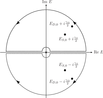
Figure 2: Integration contours in the complex $E$ plane.

$$I_{jk} =\frac{1}{2\pi}\frac{1}{E_{S,0}-E_{D,0}\pm i\,\tfrac{\gamma_{S}-\gamma_{D}}{2}}\,\Bigg{[}\frac{\gamma_{D}A_{jk}^{(S)}}{E_{S,0}-E_{D,0}\pm i\,\tfrac{\gamma_{S}+\gamma_{D}}{2}}+\frac{\gamma_{S}A_{jk}^{(D)}}{E_{S,0}-E_{D,0}\mp i\,\tfrac{\gamma_{S}+\gamma_{D}}{2}}\Bigg{]},$$ (59)

with the notation from Sec. IV.2. Here the upper (lower) signs correspond to $\Delta m_{jk}^{2}>0$ ($\Delta m_{jk}^{2}<0$). Inserting this result into Eq. (57), we obtain Eq. (41).

Appendix B Derivation of the total transition probability for the case of natural linewidth dominance

In this appendix we describe the derivation leading from Eq. (47) to Eq. (48). The spatial integrals in Eq. (47) are the same as those encountered in Sec. IV.1 and yield the factor $\exp[-{\mathbf{p}}^{2}/2\sigma_{p}^{2}]\exp[i{\mathbf{p}}{\mathbf{L}}]$. The time integrals can also be evaluated straightforwardly; however, unlike the corresponding integrals in Eq. (26), they do not give exact, but only approximate energy conserving factors for the production and detection processes. This behaviour can be ascribed to the non-zero width of the tritium states and the finite measurement time $T$. To evaluate the three-momentum integral over ${\mathbf{p}}$, we again employ the Grimus-Stockinger theorem and thus find

$$i\mathcal{A} =\frac{-i}{8\pi^{2}L}\mathcal{N}\sum_{j}\mathcal{M}_{S}^{\mu}\mathcal{M}_{D}^{\nu*}|U_{ej}|^{2}\int_{-\infty}^{\infty}\!dp_{0}\,\bar{u}_{e,S}\gamma_{\mu}(1-\gamma^{5})(\not{p}_{j}+m_{j})(1+\gamma^{5})\gamma_{\nu}u_{e,D}$$

$$\hskip 14.22636pt\cdot e^{-\frac{\gamma}{2}T}\,\frac{e^{-i(E_{S}-p_{0})T-\frac{\gamma}{2}T}-1}{p_{0}-E_{S}+i\frac{\gamma}{2}}\,\frac{e^{i(E_{D}-p_{0})T+\frac{\gamma}{2}T}-1}{p_{0}-E_{D}+i\frac{\gamma}{2}}\,\exp\bigg{[}\!-\frac{p_{0}^{2}-m_{j}^{2}}{2\sigma_{p}^{2}}\bigg{]}\,e^{i\sqrt{p_{0}^{2}-m_{j}^{2}}L},$$ (60)

where the 4-vector $p_{j}$ is defined as $p_{j}=(p_{0},(p_{0}^{2}-m_{j}^{2})^{1/2}\,{\mathbf{L}}/L)$. The exponential depending on $\sigma_{p}^{2}$, which will eventually lead to the generalized Lamb-Mössbauer factor, can be approximated by its value at $\bar{E}=(E_{S}+E_{D})/2$ because $\gamma\ll\sigma_{p}$ ensures that it is almost constant in the region from which the main contribution to the integral comes, namely the region where $|p_{0}-E_{S}|\lesssim\gamma$ and $|p_{0}-E_{D}|\lesssim\gamma$. The fact that this region is very narrow also allows us to pull the spinorial factors out of the integral and to expand the oscillation phase around $\bar{E}$:

$$i\sqrt{p_{0}^{2}-m_{j}^{2}}L\simeq i\sqrt{\bar{E}^{2}-m_{j}^{2}}L+i\frac{L}{v_{j}}(p_{0}-\bar{E})\,,$$ (61)

where $v_{j}=(\bar{E}^{2}-m_{j}^{2})^{1/2}/\bar{E}$. The integral over $p_{0}$ can then be evaluated by complex contour integration. The denominator has poles at $p_{0}=E_{S}-i\gamma/2$ and $p_{0}=E_{D}-i\gamma/2$, and the relevant terms in the numerator are

$$\Big{(}e^{-i(E_{S}-p_{0})T-\frac{1}{2}\gamma T}-1\Big{)}\Big{(}e^{i(E_{D}-p_{0})T+\frac{1}{2}\gamma T}-1\Big{)}\,e^{i(p_{0}-\bar{E})\frac{L}{v_{j}}}$$

$$\hskip 85.35826pt=\underbrace{e^{ip_{0}\frac{L}{v_{j}}}e^{-i(E_{S}-E_{D})T-\bar{E}\frac{L}{v_{j}}}}_{\textrm{(A)}}\,-\,\underbrace{e^{ip_{0}(T+\frac{L}{v_{j}})}e^{-iE_{S}T-i\bar{E}\frac{L}{v_{j}}-\frac{1}{2}\gamma T}}_{\textrm{(B)}}$$

$$\hskip 85.35826pt\phantom{=}\,-\,\underbrace{e^{-ip_{0}(T-\frac{L}{v_{j}})}e^{iE_{D}T-i\bar{E}\frac{L}{v_{j}}+\frac{1}{2}\gamma T}}_{\textrm{(C)}}\,+\,\underbrace{e^{i\frac{L}{v_{j}}p_{0}}e^{-i\bar{E}\frac{L}{v_{j}}}}_{\textrm{(D)}}.$$ (62)

To close the integration contour, we add to the real axis a half-circle of infinite radius. For the terms labeled (A), (B) and (D), this half-circle has to lie in the upper half-plane, while for (C) it has to lie in the upper half-plane for $T<L/v_{j}$, and in the lower half-plane for $T>L/v_{j}$. As the integrand is holomorphic for ${\rm Im}(p_{0})\geq 0$, only in this last case the integral can be non-zero. The residue theorem then yields

$$i\mathcal{A} =\frac{\mathcal{N}}{4\pi L}\sum_{j}\theta(T-L/v_{j})\,\mathcal{M}_{S}^{\mu}\mathcal{M}_{D}^{\nu*}|U_{ej}|^{2}\cdot\exp\bigg{[}\!-\frac{\bar{E}^{2}-m_{j}^{2}}{2\sigma_{p}^{2}}\bigg{]}\,\bar{u}_{e,S}\gamma_{\mu}(1\!-\!\gamma^{5})(\not{\bar{p}}_{j}+m_{j})(1\!+\!\gamma^{5})$$

$$\hskip 5.69046pt\cdot\gamma_{\nu}u_{e,D}e^{i\sqrt{\bar{E}^{2}-m_{j}^{2}}L}\frac{e^{-\frac{1}{2}\gamma(T-\frac{L}{v_{j}})}e^{-\frac{i}{2}(E_{S}-E_{D})T)}}{E_{S}-E_{D}}\bigg{[}e^{-\frac{i}{2}(E_{S}-E_{D})(T-\frac{L}{v_{j}})}-e^{\frac{i}{2}(E_{S}-E_{D})(T-\frac{L}{v_{j}})}\bigg{]}\,,$$ (63)

where now $\bar{p}_{j}=(\bar{E},(\bar{E}^{2}-m_{j}^{2})^{1/2}\,{\mathbf{L}}/L)$, and $\theta(x)$ is the Heaviside step function. The total probability for finding a tritium atom at the lattice site ${\mathbf{x}}_{D}$ in the detector after a time $T$ is

$$\mathcal{P}=\overline{|\mathcal{A}|^{2}}\,,$$ (64)

where the bar indicates the average over initial spins and the sum over final spins. Apart from these spin sums, no integration over the energy distributions of the initial and final state nuclei is necessary as long as only natural line broadening is taken into account, because we are dealing with transitions between discrete energy eigenstates. A straightforward evaluation of Eq. (64) yields Eq. (48).

Appendix C Weisskopf-Wigner approach to the effects of the natural line width

In this appendix we use the Weisskopf-Wigner approach Weisskopf and Wigner (1930a, b); Cohen-Tannoudji et al. (1977); Grimus et al. (1999) to derive Eq. (47), which has been the starting point for our discussion of Mössbauer neutrinos in the regime of natural linewidth dominance. In particular, our aim is to substantiate the arguments dictating the form of the exponential decay factors by an explicit derivation.

We can write the Hamiltonian of the system as $H=H_{0}+e^{iH_{0}t}H_{1}e^{-iH_{0}t}$, where $H_{1}$ is the interaction-representation weak interaction Hamiltonian and $H_{0}$ is the remainder. In general, we will not treat $H_{1}$ as a perturbation since we are ultimately interested in the depletion of unstable states over time, which cannot be adequately described in a perturbative approach.

One can write an arbitrary state as $|\psi(t)\rangle=\sum_{j}c_{j}(t)|\phi_{j}\rangle$, where $|\phi_{j}\rangle$ are the eigenstates of $H_{0}$. The Schrödinger equation then gives the evolution equations for the coefficients $c_{j}(t)$:

$$i\dot{c}_{j}(t)=\sum_{k}\langle\phi_{j}|H_{1}|\phi_{k}\rangle\,c_{k}(t)\,.$$ (65)

For our purposes it will be convenient to slightly modify the notation and classify the different states according to their particle content, as shown in Table 1.

	Particles		Energy	Coefficient	State vector
Initial state	${}^{3}{\rm H}_{S}$	${}^{3}{\rm He}_{D}$	$E^{(i)}$	$c^{(i)}$	$|\phi^{(i)}\rangle$
Intermediate states	${}^{3}{\rm He}_{S}^{+}$, $\bar{\nu}_{S}$, $e_{S}^{-}$	${}^{3}{\rm He}_{D}$	$E^{(1)}_{j}$	$c^{(1)}_{j}$	$|\phi^{(1)}_{j}\rangle$
	${}^{3}{\rm H}_{S}$	${}^{3}{\rm H}_{D}$, $\nu_{D}$	$E^{(2)}_{k}$	$c^{(2)}_{k}$	$|\phi^{(2)}_{k}\rangle$
	${}^{3}{\rm He}_{S}^{+}$, $\bar{\nu}_{S}$, $e_{S}^{-}$	${}^{3}{\rm H}_{D}$, $\nu_{D}$	$E^{(3)}_{jk}$	$c^{(3)}_{jk}$	$|\phi^{(3)}_{jk}\rangle$
	${}^{3}{\rm He}_{S}$	${}^{3}{\rm H}_{D}$	$E^{(4)}$	$c^{(4)}$	$|\phi^{(4)}\rangle$
	${}^{3}{\rm H}_{S}$	${}^{3}{\rm He}_{D}^{+}$, $\bar{\nu}_{D}$ $e^{-}_{D}$, $\nu_{D}$	$E^{(5)}_{kl}$	$c^{(5)}_{kl}$	$|\phi^{(5)}_{kl}\rangle$
	${}^{3}{\rm He}_{S}^{+}$, $\bar{\nu}_{S}$, $e_{S}^{-}$	${}^{3}{\rm He}_{D}^{+}$, $\bar{\nu}_{D}$ $e^{-}_{D}$, $\nu_{D}$	$E^{(6)}_{jkl}$	$c^{(6)}_{jkl}$	$|\phi^{(6)}_{jkl}\rangle$
Final state	${}^{3}{\rm He}_{S}$	${}^{3}{\rm He}_{D}^{+}$, $\bar{\nu}_{D}$ $e^{-}_{D}$	$E^{(f)}_{l}$	$c^{(f)}_{l}$	$|\phi^{(f)}_{l}\rangle$

Table 1: Classification of the states appearing in a Mössbauer neutrino experiment.

${}^{3}{\rm H}$ and ${}^{3}{\rm He}$ denote the two types of atoms in the experiment, and the index $S$ or $D$ shows whether the respective particle is initially localized at the source or at the detector. For those states for which we have written the electron participating in the reaction and the ${}^{3}{\rm He}^{+}$ ions separately, we imply that the electron may be either free or in an atomic bound state, while for the other states only bound electrons are considered. The upper index $(i)$ stands for the initial state, the indices $(1)$ through $(6)$ denote intermediate states, and $(f)$ stands for the final state, after the decay of the source particle, the absorption of the emitted neutrino in the detector and the decay of the produced tritium. The lower indices stand for the various quantum numbers of the particles; for example, $j$ encodes the momenta and the spins of $\bar{\nu}_{S}$ and $e_{S}^{-}$, and the information whether $e_{S}^{-}$ is bound or free.

The evolution of the system is governed by the interaction Hamiltonian $H_{1}=H_{S}^{+}+H_{D}^{-}+\tilde{H}_{D}^{+}+H.c$, where

$$H_{S}^{+} =\int\!d^{3}x\,\frac{1}{\sqrt{2}}G_{F}\cos\theta_{c}\langle{}^{3}{\rm He}|J^{\mu}|{}^{3}{\rm H}\rangle\,\bar{\psi}_{e,S}\gamma_{\mu}(1-\gamma^{5})\psi_{\nu}\,,$$ (66)

$$H_{D}^{-} =\int\!d^{3}x\,\frac{1}{\sqrt{2}}G_{F}\cos\theta_{c}\langle{}^{3}{\rm H}|J^{\mu}|{}^{3}{\rm He}\rangle\,\bar{\psi}_{\nu}\gamma_{\mu}(1-\gamma^{5})\psi_{e,D}\,,$$ (67)

$$\tilde{H}_{D}^{+} =\int\!d^{3}x\,\frac{1}{\sqrt{2}}G_{F}\cos\theta_{c}\langle{}^{3}{\rm He}|J^{\mu}|{}^{3}{\rm H}\rangle\,\bar{\psi}_{e,S}\gamma_{\mu}(1-\gamma^{5})\psi_{\nu}\,.$$ (68)

The Hermitian conjugates of these operators will be denoted $H_{S}^{-}$, $H_{D}^{+}$ and $\tilde{H}_{D}^{-}$. The Hamiltonians $H_{S}^{+}$ and $\tilde{H}_{D}^{+}$ describe tritium decay in the source and detector respectively, whereas $H_{D}^{-}$ describes the $\bar{\nu}_{e}$ capture in the detector. Although the Hamiltonians are essentially related by $H_{S}^{+}=H_{D}^{+}=\tilde{H}_{D}^{+}$, we will treat them as distinct operators throughout this appendix to keep our derivation more transparent and more general. For the matrix elements of the transitions, the following relations hold:

$$\begin{aligned} \langle\phi^{(i)}|H_{S}^{-}|\phi^{(1)}_{j}\rangle&=\langle\phi^{(2)}_{k}|H_{S}^{-}|\phi^{(3)}_{jk}\rangle=\langle\phi^{(5)}_{kl}|H_{S}^{-}|\phi^{(6)}_{jkl}\rangle,\\ \langle\phi^{(i)}|H_{D}^{+}|\phi^{(2)}_{k}\rangle&=\langle\phi^{(1)}_{j}|H_{D}^{+}|\phi^{(3)}_{jk}\rangle,\\ \langle\phi^{(4)}|\tilde{H}_{D}^{-}|\phi^{(f)}_{l}\rangle&=\langle\phi^{(2)}_{k}|\tilde{H}_{D}^{-}|\phi^{(5)}_{kl}\rangle=\langle\phi^{(3)}_{jk}|\tilde{H}_{D}^{-}|\phi^{(6)}_{jkl}\rangle,\end{aligned}$$ (69)

and similarly,

$$\begin{aligned} E^{(i)}-E^{(1)}_{j}&=E^{(2)}_{k}-E^{(3)}_{jk}=E^{(5)}_{kl}-E^{(6)}_{jkl},\\ E^{(i)}-E^{(2)}_{k}&=E^{(1)}_{j}-E^{(3)}_{jk},\\ E^{(4)}-E^{(f)}_{l}&=E^{(2)}_{k}-E^{(5)}_{kl}=E^{(3)}_{jk}-E^{(6)}_{jkl}.\end{aligned}$$ (70)

They follow from the fact that the corresponding processes differ only by the spectator particles. The evolution equations for the system are

$$i\dot{c}^{(i)} =\sum_{j}\langle\phi^{(i)}|H_{S}^{-}|\phi^{(1)}_{j}\rangle\,c^{(1)}_{j}+\sum_{k}\langle\phi^{(i)}|H_{D}^{+}|\phi^{(2)}_{k}\rangle\,c^{(2)}_{k},$$ (71)

$$i\dot{c}^{(1)}_{j} =\langle\phi^{(1)}_{j}|H_{S}^{+}|\phi^{(i)}\rangle\,c^{(i)}+\sum_{k}\langle\phi^{(1)}_{j}|H_{D}^{+}|\phi^{(3)}_{jk}\rangle\,c^{(3)}_{jk},$$ (72)

$$i\dot{c}^{(2)}_{k} =\langle\phi^{(2)}_{k}|H_{D}^{-}|\phi^{(i)}\rangle\,c^{(i)}+\sum_{j}\langle\phi^{(2)}_{k}|H_{S}^{-}|\phi^{(3)}_{jk}\rangle\,c^{(3)}_{jk}+\sum_{l}\langle\phi^{(2)}_{k}|\tilde{H}_{D}^{-}|\phi^{(5)}_{kl}\rangle\,c^{(5)}_{kl},$$ (73)

$$i\dot{c}^{(3)}_{jk} =\langle\phi^{(3)}_{jk}|H_{D}^{-}|\phi^{(1)}_{j}\rangle\,c^{(1)}_{j}+\langle\phi^{(3)}_{jk}|H_{S}^{+}|\phi^{(2)}_{k}\rangle\,c^{(2)}_{k}+\sum_{l}\langle\phi^{(3)}_{jk}|\tilde{H}_{D}^{-}|\phi^{(6)}_{jkl}\rangle\,c^{(6)}_{jkl},$$ (74)

$$i\dot{c}^{(4)} =\sum_{j}\langle\phi^{(4)}|H_{D}^{-}({t_{1}})|\phi^{(1)}_{j}\rangle\,c^{(1)}_{j}+\sum_{k}\langle\phi^{(4)}|H_{S}^{+}|\phi^{(2)}_{k}\rangle\,c^{(2)}_{k}+\sum_{l}\langle\phi^{(4)}|\tilde{H}_{D}^{-}|\phi^{(f)}_{l}\rangle\,c^{(f)}_{l},$$ (75)

$$i\dot{c}^{(5)}_{kl} =\langle\phi^{(5)}_{kl}|\tilde{H}_{D}^{+}|\phi^{(2)}_{k}\rangle\,c^{(2)}_{k}+\sum_{j}\langle\phi^{(5)}_{kl}|H_{S}^{-}|\phi^{(6)}_{jkl}\rangle\,c^{(6)}_{jkl},$$ (76)

$$i\dot{c}^{(6)}_{jkl} =\langle\phi^{(6)}_{jkl}|H_{S}^{+}|\phi^{(5)}_{kl}\rangle\,c^{(5)}_{kl}+\langle\phi^{(6)}_{jkl}|\tilde{H}_{D}^{+}|\phi^{(3)}_{jk}\rangle\,c^{(3)}_{jk},\phantom{\sum_{k}}$$ (77)

$$i\dot{c}^{(f)}_{l} =\sum_{k}\langle\phi^{(f)}|H_{S}^{+}|\phi^{(5)}_{kl}\rangle\,c^{(5)}_{kl}+\langle\phi^{(f)}_{l}|\tilde{H}_{D}^{+}|\phi^{(4)}\rangle\,c^{(4)}.$$ (78)

We treat all processes that occur within the source or within the detector non-perturbatively, while first-order perturbation theory will be used for processes that require the propagation of a neutrino between the source and the detector. This second kind of transitions is suppressed due to the smallness of the solid angle at which the detector is seen from the source. Consequently, we include only the respective forward reactions (i.e. those proceeding downward in the scheme of Table 1), but neglect the feedback terms, which would otherwise appear in the equations for $c^{(1)}_{j}$, $c^{(2)}_{k}$, and $c^{(5)}_{kl}$. The feedback of $|\phi^{(f)}_{l}\rangle$ to $|\phi^{(4)}\rangle$ is included because the production of both states from the initial state requires a single neutrino propagation between the source and the detector. The sums in Eqs. (71) – (78) symbolically denote the summation over the relevant discrete indices and integration over the continuous variables.

The initial conditions for the equation system (71) – (78) are given by $c^{(i)}(0)=1$ with all other coefficients vanishing at $t=0$.

Our ultimate goal is to solve the evolution equations for $c^{(4)}(t)$, which determines the ${}^{3}{\rm H}$ abundance in the detector at time $t$. It is convenient to first consider the closed subsystem formed by Eqs. (71), (72), (73), (74), (76) and (77), which we solve from the bottom upwards. We start by integrating Eq. (77) to obtain an expression for $c^{(6)}_{jkl}$, which we then insert into Eq. (76). This yields

$$i\dot{c}^{(5)}_{kl}(t) =\langle\phi^{(5)}_{kl}|\tilde{H}_{D}^{+}(t)|\phi^{(2)}_{k}\rangle c^{(2)}_{k}(t)$$

$$\hskip 14.22636pt-i\sum_{j}\int_{0}^{t}d{t_{1}}\,\langle\phi^{(5)}_{kl}|H_{S}^{-}(t)|\phi^{(6)}_{jkl}\rangle\,\langle\phi^{(6)}_{jkl}|H_{S}^{+}({t_{1}})|\phi^{(5)}_{kl}\rangle\,c^{(5)}_{kl}({t_{1}})$$

$$\hskip 14.22636pt-i\sum_{j}\int_{0}^{t}d{t_{1}}\,\langle\phi^{(5)}_{kl}|H_{S}^{-}(t)|\phi^{(6)}_{jkl}\rangle\,\langle\phi^{(6)}_{jkl}|\tilde{H}_{D}^{+}({t_{1}})|\phi^{(3)}_{jk}\rangle\,c^{(3)}_{jk}({t_{1}})\,.$$ (79)

Consider first the second term, which describes the effect on $|\phi^{(5)}_{kl}\rangle$ of its decay into $|\phi^{(6)}_{jkl}\rangle$. Following the Weisskopf-Wigner procedure as described in Cohen-Tannoudji et al. (1977), we split the quantum numbers indexed by $j$ into the energy $E^{(6)}$ and the remaining parameters $\beta$. Denoting the density of states (the number of states per unit energy interval) by $\rho(E^{(6)},\beta)$, one can make the replacements

$$|\phi^{(6)}_{jkl}\rangle\rightarrow|\phi^{(6)}_{kl};E^{(6)},\beta\rangle\,,\qquad\qquad\sum_{j}\rightarrow\sum_{\beta}\,\int\!dE^{(6)}\rho(E^{(6)},\beta)$$ (80)

in the second term of Eq. (79), which gives

$$-i\int\!dE^{(6)}K(E^{(6)})\,\int_{0}^{t}d{t_{1}}\,e^{i(E^{(5)}_{kl}-E^{(6)})(t-{t_{1}})}\,c^{(5)}_{kl}({t_{1}})\,.$$ (81)

Here we have explicitly written down the time dependence of the matrix elements and introduced the quantity

$$K(E^{(6)})=\sum_{\beta}\,\left|\langle\phi^{(5)}_{kl}|H_{S}^{-}(0)|\phi^{(6)}_{kl};E^{(6)},\beta\rangle\right|^{2}\,\rho(E^{(6)},\beta)\,,$$ (82)

which is a smooth (non-oscillating) function of energy. More specifically, $K(E^{(6)})$ represents a broad bump of width $\mathcal{O}(m_{W})$, so that a non-negligible contribution to the energy integral in (81) can only arise if $t-{t_{1}}\lesssim 1/m_{W}$. Otherwise, the integrand is fast oscillating and the integral is strongly suppressed. Therefore, we can to a very good accuracy replace $c^{(5)}_{kl}({t_{1}})$ by $c^{(5)}_{kl}(t)$ in Eq. (81) and pull it out of the integral over ${t_{1}}$ (we assume that $c^{(5)}_{kl}(t)$ is approximately constant over time intervals of order $1/m_{W}$. This assumption will be justified a posteriori by inspecting the obtained expression for $c^{(5)}_{kl}(t)$). For $t\gg 1/m_{W}$ we thus obtain

$$-ic^{(5)}_{kl}(t)\int\!dE^{(6)}\,K(E^{(6)})\int_{0}^{t}d{t_{1}}\,e^{i(E^{(5)}_{kl}-E^{(6)})(t-{t_{1}})}$$

$$\simeq-ic^{(5)}_{kl}(t)\int\!dE^{(6)}\bigg{[}\pi\delta(E^{(5)}_{kl}-E^{(6)})+iP\bigg{(}\frac{1}{E^{(5)}_{kl}-E^{(6)}}\bigg{)}\bigg{]}K(E^{(6)})$$

$$=-i\bigg{(}\frac{\gamma}{2}+i\delta E\bigg{)}c^{(5)}_{kl}(t)\,,$$ (83)

where

$$\gamma=2\pi K(E^{(5)}_{kl})\,,\qquad\qquad\delta E=P\int\!dE^{(6)}\frac{K(E^{(6)})}{E^{(5)}_{kl}-E^{(6)}}\,,$$ (84)

and $P$ denotes the principal value. As follows from the definition of the function $K(E)$ in Eq. (82) and Fermi’s golden rule, $\gamma$ is just the decay width of ${}^{3}{\rm H}$ in the source. The quantity $\delta E$ is the mass renormalization of the particles forming $|\phi^{(5)}_{kl}\rangle$. From now on, we will omit $\delta E$ and similar quantities in subsequent formulas, assuming that they are already included in the definition of the physical masses of the involved particles. The formal solution to Eq. (79) is

$$c^{(5)}_{kl}(t) =-i\int_{0}^{t}\!d{t_{1}}\,\langle\phi^{(5)}_{kl}|\tilde{H}_{D}^{+}({t_{1}})|\phi^{(2)}_{k}\rangle\,e^{-\frac{1}{2}\gamma(t-{t_{1}})}\,c^{(2)}_{k}({t_{1}})$$ (85)

$$\hskip 14.22636pt+(-i)^{2}\sum_{j}\int_{0}^{t}\!d{t_{1}}\int_{0}^{{t_{1}}}\!d{t_{2}}\langle\phi^{(5)}_{kl}|H_{S}^{-}({t_{1}})|\phi^{(6)}_{jkl}\rangle\,\langle\phi^{(6)}_{jkl}|\tilde{H}_{D}^{+}({t_{2}})|\phi^{(3)}_{jk}\rangle\,e^{-\frac{1}{2}\gamma(t-{t_{1}})}\,c^{(3)}_{jk}({t_{2}})\,.$$

By a similar argument, we obtain from Eq. (74):

$$i\dot{c}^{(3)}_{jk}(t) =\langle\phi^{(3)}_{jk}|H_{D}^{-}(t)|\phi^{(1)}_{j}\rangle\,c^{(1)}_{j}(t)+\langle\phi^{(3)}_{jk}|H_{S}^{+}(t)|\phi^{(2)}_{k}\rangle\,c^{(2)}_{k}(t)-i\frac{\tilde{\gamma}}{2}c^{(3)}_{jk}(t)$$

$$\hskip 14.22636pt-i\sum_{l}\int_{0}^{t}\!d{t_{1}}\,\langle\phi^{(3)}_{jk}|\tilde{H}_{D}^{-}(t)|\phi^{(6)}_{jkl}\rangle\,\langle\phi^{(6)}_{jkl}|H_{S}^{+}({t_{1}})|\phi^{(5)}_{kl}\rangle\,c^{(5)}_{kl}({t_{1}})\,,$$ (86)

where the decay width of ${}^{3}{\rm H}$ in the detector, $\tilde{\gamma}$, has been defined in analogy with Eq. (84). We will now show that the last term of Eq. (86) can be neglected. To this end, we insert in it the expression for $c^{(5)}_{kl}(t)$ from (85), which yields

$$\ (-i)^{2}\sum_{l}\int_{0}^{t}\!d{t_{1}}\int_{0}^{t_{1}}\!d{t_{2}}\,|\langle\phi^{(2)}_{k}|\tilde{H}_{D}^{-}(0)|\phi^{(5)}_{kl}\rangle|^{2}\,\langle\phi^{(6)}_{jkl}|H_{S}^{+}({t_{1}})|\phi^{(5)}_{kl}\rangle$$

$$\hskip 199.16928pt\cdot e^{i\left(E^{(2)}_{k}-E^{(5)}_{kl}\right)(t-{t_{2}})}\,e^{-\frac{1}{2}\gamma({t_{1}}-{t_{2}})}\,c^{(2)}_{k}({t_{2}})$$

$$+ \ (-i)^{3}\sum_{l}\int_{0}^{t}\!d{t_{1}}\int_{0}^{t_{1}}\!d{t_{2}}\int_{0}^{t_{2}}\!d{t_{3}}\,|\langle\phi^{(2)}_{k}|\tilde{H}_{D}^{-}(0)|\phi^{(5)}_{kl}\rangle|^{2}\,\langle\phi^{(6)}_{jkl}|H_{S}^{+}({t_{1}})|\phi^{(5)}_{kl}\rangle\sum_{j^{\prime}}\langle\phi^{(5)}_{kl}|H_{S}^{-}({t_{2}})|\phi^{(6)}_{j^{\prime}kl}\rangle\,$$

$$\hskip 199.16928pt\cdot e^{i\left(E^{(2)}_{k}-E^{(5)}_{kl}\right)(t-{t_{3}})}\,c^{(3)}_{j^{\prime}k}({t_{3}})\,.$$ (87)

Here we have used Eqs. (69) and (70). We will show now that the first term of Eq. (87) can be neglected; a similar argument can be used to justify the neglect of the second term.

Replacing the index $l$ by $E^{(5)}$ and $\tilde{\beta}$ in analogy with Eq. (80), we obtain

$$(-i)^{2}\int\!dE^{(5)}\,\tilde{K}(E^{(5)})\int_{0}^{t}\!d{t_{1}}\int_{0}^{t_{1}}\!d{t_{2}}\,\langle\phi^{(6)}_{jkl}|H_{S}^{+}({t_{1}})|\phi^{(5)}_{kl}\rangle\,e^{i\left(E^{(2)}_{k}-E^{(5)}\right)(t-{t_{2}})}\,e^{-\frac{1}{2}\gamma({t_{1}}-{t_{2}})}\,c^{(2)}_{k}({t_{2}})\,,$$ (88)

with $\tilde{K}(E^{(5)})$ defined analogously to $K(E^{(6)})$. As in Eq. (81), the energy integral is non-negligible only if $t-{t_{2}}\lesssim 1/m_{W}$. We see immediately that here this condition also implies $t-{t_{1}}\lesssim 1/m_{W}$. Consequently, we may pull out of the integral those terms which remain approximately constant over time intervals $\mathcal{O}(1/m_{W})$, which gives

$$\ (-i)^{2}\langle\phi^{(6)}_{jkl}|H_{S}^{+}(t)|\phi^{(5)}_{kl}\rangle c^{(2)}_{k}(t)\int\!dE^{(5)}\,\tilde{K}(E^{(5)})\int_{0}^{t}\!d{t_{1}}\int_{0}^{t_{1}}\!d{t_{2}}\,e^{i\left(E^{(2)}_{k}-E^{(5)}\right)(t-{t_{2}})}$$

$$\sim \ (-i)^{2}\langle\phi^{(6)}_{jkl}|H_{S}^{+}(t)|\phi^{(5)}_{kl}\rangle c^{(2)}_{k}(t)\frac{1}{m_{W}}\int\!dE^{(5)}\,\bigg{[}\pi\delta(E^{(2)}_{k}-E^{(5)})+iP\bigg{(}\frac{1}{E^{(2)}_{k}-E^{(5)}}\bigg{)}\bigg{]}\tilde{K}(E^{(5)})$$

$$\sim \ \mathcal{O}\bigg{(}\frac{\tilde{\gamma}}{m_{W}}\bigg{)},$$ (89)

which is negligible compared to the other terms contributing to $\dot{c}^{(3)}_{jk}(t)$ (cf. Eq. (86)). This result already suggests the general rule that the only transitions which may contribute sizeably to the evolution equations are those corresponding to the direct production of the states (i.e. production with a minimum number of intermediate steps), and those corresponding to direct feedback from a daughter state into its immediate parent state, e.g. from $|\phi^{(6)}_{jkl}\rangle$ into $|\phi^{(3)}_{jk}\rangle$. All terms corresponding to more complicated interaction chains are negligible. One can now solve Eq. (87) for $c^{(3)}_{jk}$:

$$c^{(3)}_{jk}(t) =-i\int_{0}^{t}\!d{t_{1}}\langle\phi^{(3)}_{jk}|H_{D}^{-}({t_{1}})|\phi^{(1)}_{j}\rangle\,e^{-\frac{1}{2}\tilde{\gamma}(t-{t_{1}})}\,c^{(1)}_{j}({t_{1}})$$

$$\hskip 14.22636pt-i\int_{0}^{t}\!d{t_{1}}\langle\phi^{(3)}_{jk}|H_{S}^{+}({t_{1}})|\phi^{(2)}_{k}\rangle\,e^{-\frac{1}{2}\tilde{\gamma}(t-{t_{1}})}\,c^{(2)}_{k}({t_{1}})\,.$$ (90)

Next, we plug our expressions (90) and (85) for $c^{(3)}_{jk}$ and $c^{(5)}_{kl}$ into Eq. (73):

$$i\dot{c}^{(2)}_{k}(t) =\langle\phi^{(2)}_{k}|H_{D}^{-}(t)|\phi^{(i)}\rangle c^{(i)}(t)-i\frac{\gamma}{2}c^{(2)}_{k}(t)-i\frac{\tilde{\gamma}}{2}c^{(2)}_{jk}(t)$$

$$\hskip 14.22636pt-i\sum_{j}\int_{0}^{t}\!d{t_{1}}\,\langle\phi^{(2)}_{k}|H_{S}^{-}(t)|\phi^{(3)}_{jk}\rangle\,\langle\phi^{(3)}_{jk}|H_{D}^{-}({t_{1}})|\phi^{(1)}_{j}\rangle\,e^{-\frac{1}{2}\tilde{\gamma}(t-{t_{1}})}\,c^{(1)}_{j}({t_{1}})\,.$$ (91)

We have omitted a term containing the product of $\langle\phi^{(2)}_{k}|\tilde{H}_{D}^{-}|\phi^{(5)}_{kl}\rangle$, $\langle\phi^{(5)}_{kl}|H_{S}^{-}|\phi^{(6)}_{jkl}\rangle$ and $\langle\phi^{(6)}_{jkl}|\tilde{H}_{D}^{+}|\phi^{(3)}_{jk}\rangle$ and thus describing the transition chain $|\phi^{(3)}_{jk}\rangle\rightarrow|\phi^{(6)}_{jkl}\rangle\rightarrow|\phi^{(5)}_{kl}\rangle\rightarrow|\phi^{(2)}_{k}\rangle$, because this term can be shown to be $\mathcal{O}(\tilde{\gamma}/m_{W})$ by an argument similar to the one we used for Eq. (89). The formal solution to Eq. (91) is

$$c^{(2)}_{k}(t) =-i\int_{0}^{t}\!d{t_{1}}\,\langle\phi^{(2)}_{k}|H_{D}^{-}({t_{1}})|\phi^{(i)}\rangle\,e^{-\frac{1}{2}\gamma(t-{t_{1}})-\frac{1}{2}\tilde{\gamma}(t-{t_{1}})}\,c^{(i)}({t_{1}})$$ (92)

$$+(-i)^{2}\sum_{j}\int_{0}^{t}\!d{t_{1}}\int_{0}^{t_{1}}\!d{t_{2}}\,\langle\phi^{(2)}_{k}|H_{S}^{-}({t_{1}})|\phi^{(3)}_{jk}\rangle\,\langle\phi^{(3)}_{jk}|H_{D}^{-}({t_{2}})|\phi^{(1)}_{j}\rangle\,e^{-\frac{1}{2}\gamma(t-{t_{1}})-\frac{1}{2}\tilde{\gamma}(t-{t_{2}})}\,c^{(1)}_{j}({t_{2}})\,.$$

We now proceed to Eq. (72):

$$i\dot{c}^{(1)}_{j}(t) =\langle\phi^{(1)}_{j}|H_{S}^{+}(t)|\phi^{(i)}\rangle c^{(i)}(t)$$

$$\hskip 14.22636pt-i\sum_{k}\int_{0}^{t}\!d{t_{1}}\,\langle\phi^{(1)}_{j}|H_{D}^{+}(t)|\phi^{(3)}_{jk}\rangle\,\langle\phi^{(3)}_{jk}|H_{D}^{-}({t_{1}})|\phi^{(1)}_{j}\rangle\,e^{-\frac{1}{2}\tilde{\gamma}(t-{t_{1}})}\,c^{(1)}_{j}({t_{1}})\,.$$ (93)

The contributions coming from $c^{(2)}_{k}$ through the transition chain $|\phi^{(2)}_{k}\rangle\rightarrow|\phi^{(3)}_{jk}\rangle\rightarrow|\phi^{(1)}_{j}\rangle$ are again omitted as being $\mathcal{O}(\tilde{\gamma}/m_{W})$. The term containing $\langle\phi^{(1)}_{j}|H_{D}^{+}(t)|\phi^{(3)}_{jk}\rangle\,\langle\phi^{(3)}_{jk}|H_{D}^{-}({t_{1}})|\phi^{(1)}_{j}\rangle$ describes the direct feedback from $|\phi^{(3)}_{jk}\rangle$ to $|\phi^{(1)}_{j}\rangle$, but since the transition $|\phi^{(1)}_{j}\rangle\to|\phi^{(3)}_{jk}\rangle$ does not occur spontaneously, the corresponding decay width is zero. Indeed, when applying the Weisskopf-Wigner procedure, we see that the resulting $\delta$-function under the energy integral is zero for all allowed energies. Thus, the second term in Eq. (93) is negligible, and the equation is solved by

$$c^{(1)}_{j}(t) =-i\int_{0}^{t}\!d{t_{1}}\,\langle\phi^{(1)}_{j}|H_{S}^{+}({t_{1}})|\phi^{(i)}\rangle\,c^{(i)}({t_{1}})\,.$$ (94)

We can insert this expression, together with $c^{(2)}_{k}(t)$ from Eq. (92), into the equation for $c^{(i)}(t)$, and find

$$c^{(i)}(t)=e^{-\frac{1}{2}\gamma t}\,,$$ (95)

up to a term suppressed by $\tilde{\gamma}/m_{W}$. The closed-form expressions for $c^{(1)}_{j}(t)$, $c^{(2)}_{k}(t)$, $c^{(3)}_{jk}(t)$, $c^{(5)}_{kl}(t)$, and $c^{(6)}_{jkl}(t)$ are then

$$c^{(1)}_{j}(t) =-i\int_{0}^{t}\!d{t_{1}}\,\langle\phi^{(1)}_{j}|H_{S}^{+}({t_{1}})|\phi^{(i)}\rangle\,e^{-\frac{1}{2}\gamma{t_{1}}}\,,$$ (96)

$$c^{(2)}_{k}(t) =-i\int_{0}^{t}\!d{t_{1}}\,\langle\phi^{(2)}_{k}|H_{D}^{-}({t_{1}})|\phi^{(i)}\rangle\,e^{-\frac{1}{2}\gamma t-\frac{1}{2}\tilde{\gamma}(t-{t_{1}})}\,,$$ (97)

$$c^{(3)}_{jk}(t) =(-i)^{2}\bigg{[}\int_{0}^{t}\!d{t_{1}}\,\langle\phi^{(1)}_{j}|H_{S}^{+}({t_{1}})|\phi^{(i)}\rangle\,e^{-\frac{1}{2}\gamma{t_{1}}}\bigg{]}\bigg{[}\int_{0}^{t}\!d{t_{1}}\,\langle\phi^{(2)}_{k}|H_{D}^{-}({t_{1}})|\phi^{(i)}\rangle\,e^{-\frac{1}{2}\tilde{\gamma}(t-{t_{1}})}\bigg{]}\,,$$ (98)

$$c^{(5)}_{kl}(t) =(-i)^{2}\int_{0}^{t}\!d{t_{1}}\int_{0}^{t_{1}}\!d{t_{2}}\,\langle\phi^{(5)}_{kl}|\tilde{H}_{D}^{+}({t_{1}})|\phi^{(2)}_{k}\rangle\,\langle\phi^{(2)}_{k}|H_{D}^{-}({t_{2}})|\phi^{(i)}\rangle\,e^{-\frac{1}{2}\gamma t-\frac{1}{2}\tilde{\gamma}({t_{1}}-{t_{2}})}\,,$$ (99)

$$c^{(6)}_{jkl}(t) =(-i)^{3}\bigg{[}\int_{0}^{t}\!d{t_{1}}\,\langle\phi^{(1)}_{j}|H_{S}^{+}({t_{1}})|\phi^{(i)}\rangle\,e^{-\frac{1}{2}\gamma{t_{1}}}\bigg{]}$$

$$\hskip 56.9055pt\cdot\bigg{[}\int_{0}^{t}\!d{t_{1}}\!\int_{0}^{t_{1}}\!d{t_{2}}\,\langle\phi^{(5)}_{kl}|\tilde{H}_{D}^{+}({t_{1}})|\phi^{(2)}_{k}\rangle\,\langle\phi^{(2)}_{k}|H_{D}^{-}({t_{2}})|\phi^{(i)}\rangle\,e^{-\frac{1}{2}\tilde{\gamma}({t_{1}}-{t_{2}})}\bigg{]}\,.$$ (100)

In the expressions for $c^{(3)}_{jk}(t)$ and $c^{(6)}_{jkl}(t)$, we have used the identity

$$\int_{0}^{t}\!d{t_{1}}\int_{0}^{t_{1}}\!d{t_{2}}=\int_{0}^{t}\!d{t_{2}}\int_{t_{2}}^{t}\!d{t_{1}}.$$ (101)

Eqs. (95) – (100) show that all coefficients are slowly varying over time intervals of order $1/m_{W}$, which provides the a posteriori justification for pulling them out of the time integrals when applying the Weisskopf-Wigner procedure.

We have now all the ingredients required to solve for $c^{(4)}(t)$. We insert Eqs. (96), (97) and (78) into Eq. (75), neglect the $\mathcal{O}(\tilde{\gamma}/m_{W})$ contribution from the reaction chain $|\phi^{(5)}_{kl}\rangle\rightarrow|\phi^{(f)}_{l}\rangle\rightarrow|\phi^{(4)}\rangle$, and apply the completeness relations

$$\sum_{j}|\phi^{(1)}_{j}\rangle\langle\phi^{(1)}_{j}|=1\,,\qquad\quad\sum_{k}|\phi^{(2)}_{k}\rangle\langle\phi^{(2)}_{k}|=1$$ (102)

to dispose of the sums over $j$ and $k$ and of the intermediate bra- and ket-vectors in the products of matrix elements. This leads us to the main result of this appendix,

$$c^{(4)}(t) =(-i)^{2}\int_{0}^{t}\!d{t_{1}}\int_{0}^{t_{1}}\!d{t_{2}}\,\langle\phi^{(4)}|\Big{[}H_{D}^{-}({t_{1}})e^{-\frac{1}{2}\tilde{\gamma}(t-{t_{1}})}\,H_{S}^{+}({t_{2}})e^{-\frac{1}{2}\gamma{t_{2}}}$$

$$\hskip 142.26378pt+H_{S}^{+}({t_{1}})e^{-\frac{1}{2}\gamma{t_{1}}}\,H_{D}^{-}({t_{2}})e^{-\frac{1}{2}\tilde{\gamma}(t-{t_{2}})}\Big{]}|\phi^{(i)}\rangle\,.$$ (103)

We see that $c^{(4)}(t)$ is given by the time-ordered product of the two interaction Hamiltonians, supplemented by the classically expected exponential decay factors. After inserting the appropriate expressions for $H_{S}^{+}$ and $H_{D}^{-}$, finally setting $\tilde{\gamma}=\gamma$ and applying the Feynman rules, Eq. (103) leads directly to Eq. (47) of Sec. IV.4.

For completeness, we also give the expression for $c^{(f)}_{l}(t)$:

$$c^{(f)}_{l}(t) =(-i)^{3}\int_{0}^{t}\!d{t_{1}}\int_{0}^{t_{1}}\!d{t_{2}}\int_{0}^{t_{2}}\!d{t_{3}}\langle\phi^{(f)}_{l}|\Big{[}\tilde{H}_{D}^{+}({t_{1}})\,H_{D}^{-}({t_{2}})e^{-\frac{1}{2}\tilde{\gamma}({t_{1}}-{t_{2}})}\,H_{S}^{+}({t_{3}})e^{-\frac{1}{2}\gamma{t_{3}}}$$

$$\hskip 142.26378pt+\tilde{H}_{D}^{+}({t_{1}})\,H_{S}^{+}({t_{2}})e^{-\frac{1}{2}\gamma{t_{2}}}\,H_{D}^{-}({t_{3}})e^{-\frac{1}{2}\tilde{\gamma}({t_{1}}-{t_{3}})}\,$$

$$\hskip 142.26378pt+H_{S}^{+}({t_{1}})e^{-\frac{1}{2}\gamma{t_{1}}}\,\tilde{H}_{D}^{+}({t_{2}})H_{D}^{-}({t_{3}})e^{-\frac{1}{2}\tilde{\gamma}({t_{2}}-{t_{3}})}\Big{]}|\phi^{(i)}\rangle\,.$$ (104)

Note that an alternative way of solving Eqs. (71) – (78) is to exploit the fact that, in the closed system formed by Eqs. (71), (72), (73), (74), (76), and (77), the processes in the source and those in the detector can be separated by using a product ansatz for the coefficients $c$. Once this subsystem is solved, $c^{(4)}$ and $c^{(f)}_{l}$ can be computed as above.

References

• Mössbauer (1958) R. L. Mössbauer, Z. Phys. 151, 124 (1958).
• Frauenfelder (1962) H. Frauenfelder, The Mössbauer effect (W. A. Benjamin Inc., New York, 1962).
• Visscher (1959) W. M. Visscher, Phys. Rev. 116, 1581 (1959).
• Kells (1983) W. P. Kells, AIP Conf. Proc. 99, 272 (1983).
• Kells and Schiffer (1983) W. P. Kells and J. P. Schiffer, Phys. Rev. C28, 2162 (1983).
• Bahcall (1961) J. N. Bahcall, Phys. Rev. 124, 495 (1961).
• Mikaelyan et al. (1967) L. A. Mikaelyan, V. G. Tsinoev, and A. A. Borovoi, Yad. Fiz. 6, 349 (1967).
• Raghavan (2005) R. S. Raghavan (2005), eprint hep-ph/0511191.
• Raghavan (2006) R. S. Raghavan (2006), eprint hep-ph/0601079.
• Minakata and Uchinami (2006) H. Minakata and S. Uchinami, New J. Phys. 8, 143 (2006), eprint hep-ph/0602046.
• Minakata et al. (2007) H. Minakata, H. Nunokawa, S. J. Parke, and R. Zukanovich Funchal, Phys. Rev. D76, 053004 (2007), eprint hep-ph/0701151.
• Bilenky et al. (2007) S. M. Bilenky, F. von Feilitzsch, and W. Potzel, J. Phys. G34, 987 (2007), eprint hep-ph/0611285.
• Bilenky (2007) S. M. Bilenky (2007), eprint arXiv:0708.0260 [hep-ph].
• Giunti and Kim (1998) C. Giunti and C. W. Kim, Phys. Rev. D58, 017301 (1998), eprint hep-ph/9711363.
• Potzel (2006) W. Potzel, Phys. Scripta T127, 85 (2006).
• Coussement et al. (1992a) R. Coussement, G. S’heeren, M. Van Den Bergh, and P. Boolchand, Phys. Rev. B 45, 9755 (1992a).
• Balko et al. (1997) B. Balko, I. W. Kay, J. Nicoll, J. D. Silk, and G. Herling, Hyperfine Int. 107, 283 (1997).
• Winter (1981) R. G. Winter, Lett. Nuovo Cim. 30, 101 (1981).
• Giunti et al. (1991) C. Giunti, C. W. Kim, and U. W. Lee, Phys. Rev. D44, 3635 (1991).
• Giunti and Kim (2001) C. Giunti and C. W. Kim, Found. Phys. Lett. 14, 213 (2001), eprint hep-ph/0011074.
• Giunti (2001) C. Giunti, Mod. Phys. Lett. A16, 2363 (2001), eprint hep-ph/0104148.
• Giunti (2004) C. Giunti, Found. Phys. Lett. 17, 103 (2004), eprint hep-ph/0302026.
• Kayser (1981) B. Kayser, Phys. Rev. D24, 110 (1981).
• Giunti et al. (1992) C. Giunti, C. W. Kim, and U. W. Lee, Phys. Lett. B274, 87 (1992).
• Kiers et al. (1996) K. Kiers, S. Nussinov, and N. Weiss, Phys. Rev. D53, 537 (1996), eprint hep-ph/9506271.
• Jacob and Sachs (1961) R. Jacob and R. G. Sachs, Phys. Rev. 121, 350 (1961).
• Sachs (1963) R. G. Sachs, Annals of Physics 22, 239 (1963).
• Giunti et al. (1993) C. Giunti, C. W. Kim, J. A. Lee, and U. W. Lee, Phys. Rev. D48, 4310 (1993), eprint hep-ph/9305276.
• Rich (1993) J. Rich, Phys. Rev. D48, 4318 (1993).
• Grimus and Stockinger (1996) W. Grimus and P. Stockinger, Phys. Rev. D54, 3414 (1996), eprint hep-ph/9603430.
• Grimus et al. (1999) W. Grimus, P. Stockinger, and S. Mohanty, Phys. Rev. D59, 013011 (1999), eprint hep-ph/9807442.
• Grimus et al. (2000) W. Grimus, S. Mohanty, and P. Stockinger, Phys. Rev. D61, 033001 (2000), eprint hep-ph/9904285.
• Cardall (2000) C. Y. Cardall, Phys. Rev. D61, 073006 (2000), eprint hep-ph/9909332.
• Beuthe (2003) M. Beuthe, Phys. Rept. 375, 105 (2003), eprint hep-ph/0109119.
• Beuthe (2002) M. Beuthe, Phys. Rev. D66, 013003 (2002), eprint hep-ph/0202068.
• Lipkin (1973) H. J. Lipkin, Quantum mechanics: New approaches to selected topics (North Holland, Amsterdam, 1973).
• (37) W. Potzel, private communication.
• Coussement et al. (1992b) R. Coussement, M. van den Bergh, G. S’heeren, and P. Boolchand, Hyperfine Int. 71, 1487 (1992b).
• Odeurs (1995) J. Odeurs, Phys. Rev. B 52, 6166 (1995).
• Odeurs and Coussement (1997) J. Odeurs and R. Coussement, Hyperfine Int. 107, 299 (1997).
• Weisskopf and Wigner (1930a) V. Weisskopf and E. P. Wigner, Z. Phys. 63, 54 (1930a).
• Weisskopf and Wigner (1930b) V. Weisskopf and E. Wigner, Z. Phys. 65, 18 (1930b).
• Cohen-Tannoudji et al. (1977) C. Cohen-Tannoudji, B. Diu, and F. Laloe, Quantum mechanics, vol. 2 (Wiley-Interscience, 1977).
• Meystre et al. (1980) P. Meystre, M. O. Scully, and H. Walther, Optics Communications 33, 153 (1980).