Modelling of the moving deformed triple contact line: influence of the fluid inertia

Abstract

For partial wetting, motion of the triple liquid-gas-solid contact line is influenced by heterogeneities of the solid surface. This influence can be strong in the case of inertial (e.g. oscillation) flows where the line can be pinned or move intermittently. A model that takes into account both surface defects and fluid inertia is proposed. The viscous dissipation in the bulk of the fluid is assumed to be negligible as compared to the dissipation in the vicinity of the contact line. The equations of motion and the boundary condition at the contact line are derived from Hamilton’s principle. The rapid capillary rise along a vertical inhomogeneous wall is treated as an example.

email] vadim.nikolayev@espci.fr http://www.pmmh.espci.fr/$\sim$vnikol

1 Introduction

In equilibrium, the wetting properties of a liquid in contact with a solid are well defined by the static contact angle $\theta_{eq}$ [1]. In the case of complete wetting ($\theta_{eq}=0$), a thin prewetting film exists in front of the bulk of the liquid and its dynamics is well understood too. For partial wetting ($\theta_{eq}\neq 0$), a difficulty arises when the triple solid-liquid-gas contact line is moving. Huh and Scriven [2] showed that the viscous flow in contact line vicinity cannot be described by the no-slip condition, i.e. zero fluid velocity at the solid wall. Indeed, since the contact line belongs at the same time to the liquid and to the solid, the contact line velocity is ambiguous. This leads to a nonphysical divergence of the hydrodynamic pressure and of the viscous dissipation at the contact line. In reality, the dissipation is anomalously large but finite.

A motion of the straight contact line is studied in the large majority of works. However, wetting dynamics experiments at partial wetting are almost inevitably submitted to an influence of surface heterogeneities that we call “defects” for the sake of brevity. On small scale, they lead to the contact line deformation; on macroscopic scale, to the contact angle hysteresis, i.e. to the difference between the advancing and receding contact angles. The contact line elasticity approach was proposed to describe the static deformation of the contact line by a localized defect [1]. It resulted in the logarithmic contact line shape, which was shown to describe correctly experimental data in the intermediate range of distances from the defect center. Obviously, the logarithmic shape fails to describe the contact line both very close to the defect and far from it where the contact line deformation needs to be finite. To obtain the correct description in the whole range, the influence of gravity [3] or the fluid mass conservation [4] needs to be taken into account.

While the static hysteresis is understood relatively well [1, 5, 6], the contact line dynamics in the presence of defects is under active discussion, see [7] for related references. The contact line speed is often presented as a function of the dynamic contact angle $\theta$ and of the static contact angle. However, an ambiguity appears in definition of this static value which should lie somewhere between the advancing and receding values of the static contact angle.

Among theoretical studies of the dynamics in the presence of defects (that we call dynamics of the “deformed contact line”) one can distinguish the papers [8, 9]. Joanny & Robbins [8] proposed a general formalism for an arbitrary contact line shape but solved it only for the straight contact line. Golestanian and Raphaël [9] used the quasi-static dynamics in conjunction with the contact line elasticity model to study the random deformation of the contact line.

To describe the effect of defects, a single phenomenological parameter $\xi$, the dissipation coefficient, was introduced [10, 3] following [11]. $\xi$ contains all the physics of the contact line motion mechanism and has to be specific to the fluid-substrate system. To introduce it into the theory, one needs to assume that (i) the viscous dissipation in the bulk of the fluid is neglected with respect to that in the contact line vicinity, and (ii) the contact line dissipation is independent of the direction of the contact line motion (advancing or receding). The energy dissipated per unit time at the contact line is then given in the lowest order of the contact line velocity $v_{n}$ (measured in the direction normal to the contact line) by the expression

$$T=\int\frac{\xi\,v_{n}^{2}}{2}\;{\rm d}l,$$ (1)

where the integration is performed along the contact line. The defects are modelled by the spatial variation of the surface energy of the support which, according to the Young-Laplace formula, is equivalent to the spatial variation of $\theta_{eq}$. It was shown in [4] that in quasistatic approximation (i.e. when the fluid surface is assumed to be at equilibrium shape at any time moment) the expression (1) leads to the equation valid for any contact line (or fluid surface) geometry,

$$v_{n}=\frac{\sigma}{\xi}(\cos\theta_{eq}-\cos\theta).$$ (2)

where $\sigma$ is the surface tension. Therefore, in any contact line motion model that results in (2), the coefficient $\xi$ can be interpreted as the contact line dissipation per its unit length. For instance, $\xi$ can be directly assimilated to the friction coefficient of Blake and Haynes [12]. The dissipation coefficient theory allows the contact line dynamics and the dynamic advancing and receding angles to be predicted once the surface heterogeneity and the initial conditions are defined [13].

The relationship (2) has been verified against multiple experiments (see [14] for a review). Using (2), the $\xi$ value can be obtained from them. According to various experimental data, $\xi$ is much larger than the shear viscosity $\eta$, which corroborates the assumption (i) above. However, there is still no certainty even about the order of value of $\xi/\eta$ for a particular liquid-solid system. The experimental values range from 300 [11] to $10^{7}$ [15] and depend on the conditions of experiment, the state of the substrate, etc.

It is argued recently [7] that $v_{n}$ is non-linear in $\cos\theta$ which is equivalent to the statement that $\xi$ varies strongly with $v_{n}$. At large $v_{n}$, the observed deviations from the behavior (2) can be explained by the model [14]. However, one needs to treat the experimental $\xi$ value at small contact speeds with caution because it is usually determined [16, 7, 17, 15] from the slope of the dependence of $\langle v_{n}\rangle$ on $\langle\cos\theta\rangle$ (where the angle brackets mean averaging along the contact line). It is shown in [13] that due to the collective effect of the defects, the dependence (2) with constant $\xi$ can result in a highly non-linear dependence of $\langle v_{n}\rangle$ on $\langle\cos\theta\rangle$ near the pinning threshold where $\langle v_{n}\rangle$ is small. The inferred from the slope $\xi$ value turns out to be larger than its actual value. The influence of defects can thus lead to averaged $v_{n}(\theta)$ equations different from (2) at small contact line speeds. To separate the effect of defects from the physics mechanism of the contact line motion, a description of the dynamics of the contact line deformed by the defects is necessary.

Most theoretical approaches aim to describe the slow fluid motion and thus neglect the fluid inertia. However, the inertial effects can be important in many common situations. One can mention the early stages of drop spreading [18], possibly after its impact with a support [19], the capillary rise [20, 21, 22], and oscillating flows in various geometries: those of sessile or pendant drops [23, 24, 25, 26, 27], liquid in containers [28, 29, 30, 31], or capillary bridges [32].

In the partial wetting regime all these situations involve a period of time where $v_{n}$ is small and then the defect impact on dynamics is large. Indeed, $v_{n}$ necessarily passes through zero during oscillations. As for relaxation processes, the influence of defects becomes important at the end of the evolution.

This problem is especially important for oscillation flows where the choice of the boundary conditions at the solid walls is a longstanding problem [28]. Evidently, when the amplitude of oscillations is small enough, the contact line is pinned [24], so that the fixed position boundary condition need to be applied. When the amplitude is larger, the contact line can be pinned during a part of the oscillation period [29, 30]. At large amplitude, it moves almost all the time. In the relatively well studied [26, 31] first regime, there is no singularity at the contact line. The transition from the first to the second regime and especially the complicated dynamics in the second regime did not yet find its explanation. In this paper we develop a model suitable to solve these problems.

The equations of motion are derived in the “shallow water” approximation in sections 2 and 3. This approximation permits to solve analytically a model problem (section 4) in order to validate the model and find a first-order “inertial” correction to the quasi-static behavior. The results are summarized in the section 5.

2 Equations of motion

The oscillating flows are considered often in the inviscid fluid approximation [31, 27]. This is justified by the thinness of the viscous boundary model at moderate Reynolds numbers where the flow is not yet turbulent. For the contact line problems, an additional argument related to the anomalously strong contact line dissipation can be put forward. Indeed the experiments [28, 29, 24, 30] show that its contribution can be larger than that of the viscosity in the liquid bulk. Therefore, we will neglect the viscous dissipation in the bulk by assuming that the liquid is inviscid. The only source of dissipation is assumed to be at the contact line.

A Cartesian reference frame $Oxyz$ is used to describe the fluid motion in the domain $x>0$, $-\infty<y<\infty$, $0<z<h(t,x,y)$ (Fig. 1). The free surface is described by the equation $z=h(t,x,y)$ and is assumed to be weakly deformed

$$|\nabla h|\ll 1,$$ (3)

where the gradient is taken with respect to the variables $(x,y)$. The vertical wall ($x=0$) may move in $z$ direction. The gravity is directed downward. The contact line is described by the equation

$$z=h_{w}(t,y)=h(t,0,y).$$ (4)

Figure 1: Sketch of the liquid layer near the vertical (possibly moving with the speed $v$) wall with surface defects.

For convenience, the function $h(t,x,y)$ is assumed to be periodic (with the period $2L$) in the $y$-direction. This is not a restrictive assumption since one might put $L\rightarrow\infty$ in the resulting equations.

To derive the governing equations and boundary conditions in the absence of the volume dissipation, we use the Hamilton principle of stationary action. The idea is to formulate the Lagrangian, and to present the variation of the Hamilton action as a linear functional of virtual displacements allowing to find not only the governing equations but also the natural boundary conditions [33, 34].

In the present work, we will use the “shallow water” approximation which will allow the analytical results to be obtained and analyzed. The Hamilton action $a$ and the Lagrangian $\mathcal{L}$ (which is the difference between the kinetic and the potential energy of the system) read

$$a=\int_{t_{1}}^{t_{2}}\mathcal{L}\,\textrm{d}t,\quad\mathcal{L}=\frac{1}{2L}\int_{0}^{\infty}\textrm{d}x\int_{-L}^{L}\left(\frac{\rho h\left|\vec{u}\right|^{2}}{2}-\frac{\rho gh^{2}}{2}\right)\textrm{d}y-$$

$$\frac{\sigma}{2L}\int_{0}^{\infty}\textrm{d}x\int_{-L}^{L}\left(\sqrt{1+|\nabla h|^{2}}-1\right)\textrm{d}y+\frac{\sigma}{2L}\int_{-L}^{L}\textrm{d}y\int_{0}^{h_{w}(t,y)}c(y,z)\,\textrm{d}z.$$ (5)

Here $\rho$ is the density of the fluid assumed incompressible, $\vec{u}=(u_{x},u_{y})$ is the fluid velocity field. The first integral in the Lagrangian is a difference between the kinetic and the gravitational potential energy of the system written in the shallow water approximation. The second integral is the liquid-gas interface energy, and the last integral is the energy of the fluid-solid surface [5], $\sigma c(y,z)$ being the difference between the interfacial tension of gas-solid and liquid-solid interfaces. According to the Young expression, $c(y,z)={\rm cos}(\theta_{eq})$, where $\theta_{eq}$ is the value of the equilibrium contact angle. The variation of the latter along the substrate (i. e. along the $y-z$ plane) reflects the surface heterogeneity (surface defects).

The variation of the action is taken under the mass conservation constraint

$$\frac{\partial h}{\partial t}+\nabla\cdot(h\vec{u})=0$$ (6)

and the non-penetration boundary condition at the vertical wall

$$\left.u_{x}\right|_{x=0}=0.$$ (7)

Search of the extremum for the action $a$ (see Appendix A) results in the following fluid motion equation:

$$\frac{\partial\left(\rho h\vec{u}\right)}{\partial t}+\nabla\cdot(\rho h\vec{u}\otimes\vec{u})+\rho gh\nabla h-\sigma h\nabla(\Delta h)=0.$$ (8)

Its back substitution into the Lagrangian (5) reduces the latter to the form (see also (42))

$$\delta\mathcal{L}=\frac{\sigma}{2L}\int_{-L}^{L}\left[\left.\frac{\partial h}{\partial x}\right|_{x=0}+c(y,h_{w})\right]\delta h_{w}\,\textrm{d}y.$$ (9)

The dissipation is introduced [3] in the usual way through the dissipation functional, (1). For this, we need to find an expression for the normal velocity $v_{n}$ of the contact line. When the vertical wall moves vertically with respect to the reference system with the velocity $v$, the velocity of the contact line with respect to the wall reads

$$v_{n}=\left(\frac{\partial h_{w}}{\partial t}+v\right)\left[1+\left(\frac{\partial h_{w}}{\partial y}\right)^{2}\right]^{-1/2}\simeq\frac{\partial h_{w}}{\partial t}+v,$$

where $v$ is assumed to be positive for the downward plate motion. Since the volume dissipation inside the fluid is neglected, the dissipation functional does not depend on the bulk fluid velocity $\vec{u}$ and the dissipation account does not influence the governing equation (8).

Following [3], one can write now the generalized Euler-Lagrange equation which takes into account the dissipation term

$$\frac{d}{dt}\left(\frac{\delta{\mathcal{L}}}{\delta\dot{h}_{w}}\right)-\frac{\delta{\mathcal{L}}}{\delta h_{w}}=-\frac{\delta T}{\delta\dot{h}_{w}},$$ (10)

where $\delta\ldots/\delta\ldots$ means functional derivative and $\dot{h}_{w}$ denotes the time derivative. The substitution of (9) into (10) results in the equation

$$\sigma\left[\left.\frac{\partial h}{\partial x}\right|_{x=0}+c(y,h_{w})\right]=\xi\left(\frac{\partial h_{w}}{\partial t}+v\right)$$ (11)

that defines the contact line position $h_{w}$. Eq. (11) plays a role of the boundary condition for the momentum equation (8).

Let us note that the shallow water approximation is not necessary to obtain the main result (11). It is known [34] that if the full Lagrangian (involving the integration over $z$ of the kinetic energy) is used instead of its “shallow water” counterpart (5), the classical Euler equation of motion for the inviscid fluid result is obtained instead of the equation (8). The back substitution into the Lagrangian would lead to the same expression (9), which is necessary to obtain Eq. (11).

3 Reduction of governing equations

The boundary conditions for the governing equations (6, 8) should be completed by the condition at infinity

$$h|_{x\rightarrow\infty}=d,$$ (12)

where $d$ is the constant depth. The following initial conditions will be used,

$$\vec{u}|_{t=0}=0,\quad h|_{t=0}=d.$$ (13)

The governing equations written for the deviation from the initial state $\hat{h}=h-d$ can be linearized:

$$\frac{\partial\hat{h}}{\partial t}+d\nabla\cdot\vec{u}=0,\quad\rho\frac{\partial\vec{u}}{\partial t}+\rho g\nabla\hat{h}-\sigma\nabla\Delta\hat{h}=0.$$ (14)

The velocity $\vec{u}$ is eliminated from these equations by applying the time derivative to the first of them and subtracting the divergence of the second. The result reads

$$\rho\frac{\partial^{2}\hat{h}}{\partial t^{2}}-\rho gd\Delta\hat{h}+\sigma d\Delta^{2}\hat{h}=0.$$ (15a)

Evidently, the first time-dependent term of this equation is inertial. Two other terms correspond to the gravity and to the surface tension contributions respectively. Without the first term, Eq. (15a) would reduce to the quasistatic linearized equation for the interface shape [3].

The boundary and initial conditions for (15a) are obtained from (7, 12–13) by using (14):

$$\hat{h}|_{x\rightarrow\infty}=0,$$ (15b)

$$\left.\frac{\partial}{\partial x}\left(\rho g\hat{h}-\sigma\Delta\hat{h}\right)\right|_{x=0}=0,$$ (15c)

$$\hat{h}|_{t=0}=0,$$ (15d)

$$\left.\frac{\partial\hat{h}}{\partial t}\right|_{t=0}=0,$$ (15e)

The nonlinear equation (11) rewritten for $\hat{h}$

$$\frac{\partial\hat{h}_{w}}{\partial t}+v=\frac{\sigma}{\xi}\left[\left.\frac{\partial\hat{h}}{\partial x}\right|_{x=0}+c(y,h_{w})\right],$$ (15f)

where $\hat{h}_{w}=h_{w}-d$, closes the problem statement.

Only the solution for $h_{w}(t,y)$ is of interest. However, it can only be obtained by analyzing the full problem (15) for $h$. The set of equations (15) allows $h_{w}$ to be obtained for arbitrary distribution of the surface defects $c(y,z)$.

4 Solution of a model problem

To demonstrate the applicability of the developed formalism, let us solve a problem of the capillary rise on an immobile ($v=0$) wall with a single stripe defect (see Fig. 3 below)

$$c(y)=\left\{\begin{array}[]{cc}c_{d},&|y|\leq w,\\ c_{s},&|y|>w,\end{array}\right.$$ (16)

where $c_{d},c_{s}$ and $w$ are constants, i.e. for the simplest case in which $c$ is independent of $z$. The values of $c_{d}$ and $c_{s}$ are the cosines of the equilibrium contact angles inside and outside the stripe defect respectively, $w$ being its half-width. This problem has already been solved in quasi-static approximation [3] (in which the fluid motion is neglected). We choose the same setup to show the role of the fluid inertia by comparing the quasi-static and inertial solutions.

Since $z$ dependence in (16) is absent, the problem (15) becomes linear. Following [3], $h$ and $h_{w}$ are broken into parts:

$$\begin{array}[]{c}h=d+h_{0}(t,x)+h_{1}(t,x,y),\\ h_{w}=d+h_{w0}(t)+h_{w1}(t,y),\\ \end{array}$$ (17)

where $h_{0}$ and $h_{w0}$ are the averaged over the $y$-direction values of $\hat{h}$ and $\hat{h}_{w}$ respectively. The problems for $h_{0}$ and $h_{1}$ are decoupled and can be solved separately.

4.1 Solution for $h_{w0}$

Consider first the problem for $h_{0}$ that can be obtained from (15) by accounting for the fact $\partial h_{0}/\partial y\equiv 0$. By applying the Laplace transform

$$\bar{h}_{0}(x)=\int_{0}^{\infty}h_{0}(t,x)\exp(-st)\,\textrm{d}t,$$ (18)

one obtains from (15a,d,e) the ordinary differential equation

$$\frac{d^{4}\bar{h}_{0}}{dx^{4}}-2\alpha\frac{d^{2}\bar{h}_{0}}{dx^{2}}+\beta\bar{h}_{0}=0,$$ (19)

where $\alpha=\rho g/(2\sigma)$, $\beta=\rho s^{2}/(\sigma d)$. The general solution of (19) has a form

$$\bar{h}_{0}(x)=a_{1}\exp(-p_{1}x)+a_{2}\exp(-p_{2}x)+a_{3}\exp(p_{1}x)+a_{4}\exp(p_{2}x),$$ (20)

where

$$p_{1,2}=\sqrt{\alpha\pm\sqrt{\alpha^{2}-\beta}},\quad\mbox{Re}\;p_{1,2}\geq 0.$$ (21)

The boundary conditions for $\bar{h}_{0}$ have the same form (15b,c) as for $h_{0}$; (15f) transforms into

$$s\bar{h}_{w0}=\frac{\sigma}{\xi}\left(\left.\frac{d\bar{h}_{0}}{dx}\right|_{x=0}+\frac{c_{s}}{s}\right),$$ (22)

where $\bar{h}_{w0}$ is the Laplace transform of $h_{w0}$. Because of (15b),

$$a_{3}=a_{4}=0,$$ (23)

and (15c) results in the following condition

$$\left.\frac{d\bar{h}_{0}}{dx}\right|_{x=0}=-\bar{h}_{w0}(p_{1}+p_{2})=-\bar{h}_{w0}\sqrt{2\left(\alpha+\sqrt{\beta}\right)}.$$ (24)

The final form for $\bar{h}_{w0}$ can be obtained by the substitution of (24) into (22):

$$\bar{h}_{w0}=c_{s}\frac{\sigma}{\xi}\left[s\left(s+\tau_{r}^{-1}\sqrt{s\sqrt{2\tau_{i}}+1}\right)\right]^{-1},$$ (25)

where $\tau_{r}=l_{c}\xi/\sigma$ is a characteristic time scale for the quasi-static relaxation [3] and $\tau_{i}=l_{c}/\sqrt{gd}$ is the characteristic inertial time, $l_{c}=\sqrt{\sigma/(\rho g)}$ being the capillary length. The inverse Laplace transform of (25) can be found rigorously as described in Appendix. It reads

$$h_{w0}(t)=c_{s}l_{c}\bigg{\{}1-\mbox{erfc}\left(\sqrt{\frac{t}{2\tau_{i}}}\right)+$$

$$\frac{1}{2\sqrt{1+r^{2}}}\bigg{\{}\exp\left[\frac{t}{\tau_{r}}\left(r+\sqrt{1+r^{2}}\right)\right]\mbox{erfc}\left[\sqrt{\frac{t}{2\tau_{i}}}\left(r+\sqrt{1+r^{2}}\right)\right]-$$

$$\exp\bigg{[}\frac{t}{\tau_{r}}\bigg{(}r-\sqrt{1+r^{2}}\bigg{)}\bigg{]}\mbox{erfc}\left[\sqrt{\frac{t}{2\tau_{i}}}\left(r-\sqrt{1+r^{2}}\right)\right]\bigg{\}}\bigg{\}},$$ (26)

where $\mbox{erfc}(\cdot)$ is the complementary error function [35], and $r=\tau_{i}/\tau_{r}$ characterizes a relative importance of the fluid inertia. It is related to the Weber number which can be obtained from (15a) where both the terms of inertia and of surface tension are present. Taking $\tau_{r}$ and $l_{c}$ as the scales of time and length, one can obtain for these terms $\rho h/\tau_{r}^{2}$ and $\sigma dh/l_{c}^{4}$. Their ratio is the Weber number, $We=r^{2}$.

In the limit $r\rightarrow 0$, (4.1) reduces to the quasi-static result [3]

$$h_{w0}(t)|_{r\rightarrow 0}=c_{s}l_{c}[1-\exp(-{t}/{\tau_{r}})].$$ (27)

The difference between these two dependencies is transparent from Fig. 2: the fluid inertia slightly slows down the contact line relaxation. For $r\leq 0.01$, the difference between the functions (4.1) and (27) is very small so that in practice the exponential solution (27) is valid.

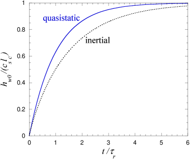
Figure 2: The time dependence of the $y$-averaged hight of the contact line rise $h_{w0}$. The exponential quasi-static law (27) (solid line) is compared to the inertial behavior (4.1) (dotted line) calculated for $r=0.5$.

4.2 Solution for $h_{w1}$

The statement of the problem for $h_{1}$ is given by (15) with an additional condition of zero $y$-averaged value of $h_{1}$. For a single defect, this condition reduces to $h_{1}(y\rightarrow\pm\infty)=0$, which allows the Fourier transform

$$\tilde{h}_{1}(t,x)=\int_{-\infty}^{\infty}h_{1}(t,x,y)\exp(-iky)\,\textrm{d}y$$ (28)

to be applied. The Laplace transform (18) can further be applied to $\tilde{h}_{1}(t,x)$ and results in $\bar{h}_{1}(x)$.

The further procedure is fully analogous to that developed in the previous section. It leads to the following equation for $\bar{h}_{w1}$

$$s\bar{h}_{w1}=\frac{\sigma}{\xi}\left(\left.\frac{d\bar{h}_{1}}{dx}\right|_{x=0}+\frac{\tilde{c}_{1}}{s}\right),$$ (29)

where $\tilde{c}_{1}$ is the Fourier transform of $c(y)-c_{s}$,

$$\tilde{c}_{1}=2\delta c\frac{\sin kw}{k},$$ (30)

and $\delta c=c_{d}-c_{s}$. The $\bar{h}_{1}$ derivative is related to $\bar{h}_{w1}$ through

$$\left.\frac{d\bar{h}_{1}}{dx}\right|_{x=0}=-\bar{h}_{w1}\frac{p_{1}p_{2}(p_{1}+p_{2})}{k^{2}+p_{1}p_{2}},$$ (31)

where $p_{1,2}$ are defined by (21), in which

$$\alpha=\frac{\rho g}{2\sigma}+k^{2},\quad\beta=\frac{\rho}{\sigma d}s^{2}+\frac{\rho g}{\sigma}k^{2}+k^{4}$$ (32)

should now be used. The substitution of (31) into (29) leads to an expression, for which the inverse Laplace transform is difficult to find. To overcome this difficulty, one can make use of the smallness of the parameter $r$, i.e. assume the smallness of the contribution of the inertial effects. In this limit, (31) reduces to

$$\left.\frac{d\bar{h}_{1}}{dx}\right|_{x=0}=-\bar{h}_{w1}\left[\sqrt{k^{2}+l_{c}^{-2}}+B(r\tau_{r}s)^{2}\right],$$ (33)

where the coefficient $B$ is

$$B=\frac{k^{2}+l_{c}^{-2}}{|k|}-\frac{k^{2}+1.5l_{c}^{-2}}{\sqrt{k^{2}+l_{c}^{-2}}}.$$ (34)

Note that $B$ is positive and diverges at small $k$ like $B\sim|k|^{-1}$. The equation for $\bar{h}_{w1}$ becomes

$$\bar{h}_{w1}=\tilde{c}_{1}\left[s\left(\sqrt{k^{2}+l_{c}^{-2}}+l_{c}^{-1}\tau_{r}s+B(r\tau_{r}s)^{2}\right)\right]^{-1}.$$ (35)

This expression is rational in $s$ and its inverse Laplace transform can be found using conventional methods:

$$\tilde{h}_{w1}(t)=\tilde{c}_{1}\left\{\frac{1}{\sqrt{k^{2}+l_{c}^{-2}}}+\frac{1}{B(r\tau_{r})^{2}(s_{1}-s_{2})}\left[\frac{\exp(s_{1}t)}{s_{1}}-\frac{\exp(s_{2}t)}{s_{2}}\right]\right\}.$$ (36)

Here

$$s_{1,2}=\frac{1\pm\sqrt{1-4Bl_{c}r^{2}\sqrt{k^{2}l_{c}^{2}+1}}}{2Bl_{c}r^{2}\tau_{r}}.$$ (37)

To obtain the time-varying contact line shape $h_{w1}(t,y)$, one needs to apply the inverse Fourier transform to (36). It can be done numerically. The result is shown in Fig. 3.

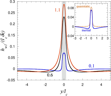
Figure 3: The contact line distortion $h_{w1}$ calculated for $r=0.5$. The defect area (half-width of which is $w=0.2l_{c}$) with $\cos\theta_{eq}=c_{d}$ is shadowed. The rest of the plane has $\cos\theta_{eq}=c_{s}$. The parameter of the curves is the time $t$ in the $\tau_{r}$ units. In the insert, the result of the inertial theory for $r=0.5$ (solid curve) is compared to the quasi-static ($r\rightarrow 0$) result (dotted curve). Both curves are calculated for $t=0.1\tau_{r}$.

At $r\rightarrow 0$, one recovers the quasi-static result [3]

$$\tilde{h}_{w1}(t)|_{r\rightarrow 0}=\frac{\tilde{c}_{1}}{\sqrt{k^{2}+l_{c}^{-2}}}\left[1-\exp\left(-\frac{t}{\tau_{r}}\sqrt{k^{2}l_{c}^{2}+1}\right)\right],$$ (38)

which corresponds to a non-zero value at $k\rightarrow 0$. However, by considering the small $k$ limit of (36), one arrives to the result

$$\tilde{h}_{w1}(t)|_{k\rightarrow 0}=\frac{\tilde{c}_{1}t^{2}}{2B\tau_{i}^{2}}\rightarrow 0.$$ (39)

This small $k$ ambiguity leads to a small but regular numerical error in $h_{w1}(t,y)$ when the inverse Fourier transform of (36) is found at very small $r$. In practice, the expression (38) should be used instead for $r\leq 0.05$.

Similarly to the case of ${h}_{w0}$, the inertial slowing down manifests itself in the case of ${h}_{w1}$. The insert in Fig. 3 shows that the topmost point of the contact line rises slower when the hydrodynamic motion is taken into account. However, the hydrodynamic effects are not limited to the simple slowing down, they change the shape of the contact line deformation. In the beginning of the capillary rise, the joint effect of the inertia and fluid mass conservation creates two wells in the ${h}_{1}$ shape (Fig. 3) from which the fluid flows off to form a bump in the middle. Later on, these cavities become more and more shallow and wide until they disappear in the equilibrium static contact line shape [3].

5 Results and discussion

The main result of the present paper is a model that allowed to describe the inertial regimes of the contact line motion whenever the impact of surface defects is important in the partial wetting regime, e.g. the pinning-depinning of the contact line during its oscillation. The equations of motion were derived for the plane vertical wall geometry and can be applied for the arbitrary defect pattern and both for the spontaneous and forced contact line motion. The hydrodynamic shallow water approximation was used to obtain the solution in the closed analytical form. However, this approach can be easily generalized to any geometry and fluid depth.

Indeed, let us have a closer look to the equation (11). Its most interesting feature is its invariance. In the hydrodynamic theory, it has exactly the same form as in the quasi-static theory [13]. Since $c(y,z)=\cos[\theta_{eq}(y,z)]$ and $\partial h/\partial x|_{x=0}\simeq-\cos\theta$ under the assumption (3), one notices that (11) is nothing else than the equation (2). It was derived under the assumption of the small deformation of the straight contact line. By analogy with the quasistatic result [4], it is however reasonable to assume that (2) is valid for any contact line deformation. Any contact line inertial problem can thus be solved by applying the Euler set of equations for the inviscid fluid with the boundary condition (2) where $\theta_{eq}(y,z)$ models the surface heterogeneity.

The asymptotics of the capillary rise at small times which follows from the present model can be compared to the available experimental data. It stems from the equation (2) that $v_{n}$ is constant at $t=0$ because $\theta(t=0)$ is fixed by the initial condition for $h$. Since $h(t=0)=0$ has been chosen, $\theta(t=0)=\pi/2$ and $h(t)\sim t$ at small times independently of the geometry of the problem. This asymptotics agrees with the results [21] on the capillary rise between flat walls. The asymptotics $h(t)\sim t^{3/2}$ obtained for the complete wetting case [36, 20] cannot be compared to our model restricted to the partial wetting. As a matter of fact, due to existence of the prewetting film [1], the contact line dissipation anomaly is much weaker for the complete wetting. The kinetics of the capillary rise is thus defined by the balance of the surface tension and inertia [20] which results in $h(t)\sim t^{3/2}$.

The effect of inertia on the contact line relaxation is two-fold. First, it is the slowing down of the average contact line motion. When the contact line speed is inhomogeneous, the inertia amplifies its variation along the contact line.

The impact of the inertia on the contact line relaxation can be measured by the value $r=\tau_{i}/\tau_{r}$ of the ratio of two characteristic times. The first of them is the inertial time and the second is the quasi-static relaxation time. The quasi-static result is recovered in the limit $r\rightarrow 0$. Note that the Weber number (the ratio of the inertial and surface tension terms) is related to $r$: $We=r^{2}$.

The simplicity of the developed approach is its main advantage. It uses a single phenomenological parameter (the contact line dissipation coefficient $\xi$) and allows complicated three dimensional problems to be treated. In this article we analyzed the contact line motion in presence of a stripe defect. This model can be directly verified against experiments [37, 38, 39]. However, the information presented in these papers is insufficient for a direct comparison and additional measurements are necessary.

Appendix A Derivation of the governing equation (8)

Assumption (3) permits us to rewrite (5) in a simpler form

$$\mathcal{L}=\frac{1}{2L}\int_{0}^{\infty}\textrm{d}x\int_{-L}^{L}\left(\frac{\rho h\left|\vec{u}\right|^{2}}{2}-\frac{\rho gh^{2}}{2}\right)\textrm{d}y-$$

$$\frac{\sigma}{2L}\int_{0}^{\infty}\textrm{d}x\int_{-L}^{L}\frac{\left|\nabla h\right|^{2}}{2}\,\textrm{d}y+\frac{\sigma}{2L}\int_{-L}^{L}\textrm{d}y\int_{0}^{h_{w}(t,y)}c(y,z)\,\textrm{d}z$$ (40)

The variation of the Lagrangian (40) submitted to the constraint (6) is taken in several steps. First, we introduce a smooth one-parameter family of virtual motions

$$\vec{x}=\vec{\Phi}(t,\vec{X},\varepsilon),\quad\vec{x}=(x,y)$$

($\vec{X}$ stands for the Lagrangian coordinates, $\varepsilon$ is a small parameter in the vicinity of zero and $\vec{x}={\mbox{\boldmath$\varphi$}}(t,\vec{X})=\vec{\Phi}(t,\vec{X},0)$ is the real motion). Then, we define the virtual displacements as functions of $(t,\vec{X})$:

$$\delta\vec{x}(t,\vec{X})=\left.\frac{\partial\vec{\Phi}(t,\vec{X},\varepsilon)}{\partial\varepsilon}\right|_{\varepsilon=0}.$$

Later, we consider the virtual displacements as functions of ($t,\vec{x}$) due to the possibility to invert $\vec{X}$ through $\vec{X}={\mbox{\boldmath$\varphi$}}^{-1}(t,\vec{x})$. The variations of the free surface $h(t,\vec{x})$ and the velocity field $\vec{u}(t,\vec{x})$ compatible with the mass conservation law (6) are given in the motion space ($t,\vec{x}$) by (see, for example, [34] or [40])

$$\delta h(t,\vec{x})=-\nabla\cdot(h\delta\vec{x}),\quad\delta\vec{u}(t,\vec{x})=\frac{d\delta\vec{x}}{dt}-\frac{\partial\vec{u}}{\partial\vec{x}}\delta\vec{x}.$$ (41)

Here

$$\frac{d}{dt}=\frac{\partial}{\partial t}+\vec{u}\cdot\nabla$$

is the material time derivative. Finally, the expression of the variation of $a$ in terms of the virtual displacements reads

$$2L\delta a=\int_{t_{1}}^{t_{2}}\textrm{d}t\int_{0}^{\infty}\textrm{d}x\int_{-L}^{L}\bigg{[}-\nabla\cdot(h\delta\vec{x})\frac{\rho\left|\vec{u}\right|^{2}}{2}+\rho h\vec{u}\cdot\left(\frac{d\delta\vec{x}}{dt}-\frac{\partial\vec{u}}{\partial\vec{x}}\delta\vec{x}\right)+$$

$$\rho gh\nabla\cdot(h\delta\vec{x})\bigg{]}\textrm{d}y+\sigma\int_{t_{1}}^{t_{2}}dt\int_{0}^{\infty}\textrm{d}x\int_{-L}^{L}\nabla h\cdot\nabla\left[\nabla\cdot(h\delta\vec{x})\right]\textrm{d}y+$$

$$\sigma\int_{t_{1}}^{t_{2}}\textrm{d}t\int_{-L}^{L}c(y,h_{w})\delta h_{w}\,\textrm{d}y.$$

By integrating by parts, accounting for the periodicity in $y$-direction, and the boundary condition (7) in the form

$$\left.\delta\vec{x}\cdot\vec{n}\right|_{x=0}=0,$$

where $\vec{n}=(1,0)$ is the unit normal vector to the plane $x=0$, we obtain

$$2L\delta a=\int_{t_{1}}^{t_{2}}\textrm{d}t\int_{0}^{\infty}\textrm{d}x\int_{-L}^{L}\left[-\frac{\partial\left(\rho h\vec{u}\right)}{\partial t}-\nabla\cdot(\rho h\vec{u}\otimes\vec{u})-h\nabla(\rho gh)+\sigma h\nabla(\Delta h)\right]\cdot\delta\vec{x}\textrm{d}y+$$

$$\sigma\int_{t_{1}}^{t_{2}}\textrm{d}t\int_{0}^{\infty}\textrm{d}x\int_{-L}^{L}\nabla\cdot\left[\nabla\cdot(h\delta\vec{x})\nabla h\right]\textrm{d}y+\sigma\int_{t_{1}}^{t_{2}}\textrm{d}t\int_{-L}^{L}c(t,y,h_{w})\delta h_{w}\textrm{d}y,$$

where $\otimes$ denotes the direct product of the vectors. The definition of $\delta h_{w}$

$$\delta h_{w}=-\left.\nabla\cdot(h\delta\vec{x})\right|_{x=0}$$

gives us the final expression for the variation of the Hamilton action:

$$2L\delta a=\int_{t_{1}}^{t_{2}}\textrm{d}t\int_{0}^{\infty}\textrm{d}x\int_{-L}^{L}\bigg{[}-\frac{\partial\left(\rho h\vec{u}\right)}{\partial t}-\nabla\cdot(\rho h\vec{u}\otimes\vec{u})-h\nabla(\rho gh)$$

$$+\sigma h\nabla(\Delta h)\bigg{]}\cdot\delta\vec{x}\,\textrm{d}y+\sigma\int_{t_{1}}^{t_{2}}\textrm{d}t\int_{-L}^{L}[\nabla h\cdot\vec{n}+c(y,h_{w})]\delta h_{w}\,\textrm{d}y.$$ (42)

The variations $\delta\vec{x}$ and $\delta h_{w}$ are independent and the term containing $\delta\vec{x}$ is absent in the dissipation function because of neglect of the viscosity in the bulk of the fluid. Therefore, the integral containing $\delta\vec{x}$ in (42) has to be equal to zero, which results in the governing equation (8).

Appendix B Laplace-inversion of (25)

The expression (25) has a form

$$\bar{f}(s)=[s(s+2b\sqrt{s+m^{2}})]^{-1},$$ (43)

for which the inverse Laplace transform is sought. The inverse of

$$\bar{f}(s-m^{2})=\frac{1}{2m^{2}b}\left[\frac{1/2}{\sqrt{s}-m}+\frac{1/2}{\sqrt{s}+m}-\frac{u_{2}(u_{2}-u_{1})^{-1}}{\sqrt{s}-u_{1}}-\frac{u_{1}(u_{1}-u_{2})^{-1}}{\sqrt{s}-u_{2}}\right],$$ (44)

where

$$u_{1,2}=-b\pm\sqrt{b^{2}+m^{2}},$$ (45)

is found using the inverse of $(\sqrt{s}+m)^{-1}$ listed in the tables [35]. To find the inverse of $\bar{f}(s)$, the original of $\bar{f}(s-m^{2})$ should be multiplied by $\exp(-m^{2}t)$ according to the rules of the Laplace transform.

References

- [1] P.-G. de Gennes, Wetting: statics and dynamics, Rev. Mod. Phys. 57 (1985) 827 – 863.
- [2] C. Huh, L. E. Scriven, Hydrodynamic model of steady movement of a solid/liquid/fluid contact line, J. Colloid Interf. Sci. 35 (1971) 85 – 101.
- [3] V. S. Nikolayev, D. A. Beysens, Equation of motion of the triple contact line along an inhomogeneous surface, Europhysics Lett. 64 (6) (2003) 763 – 768.
- [4] S. Iliev, N. Pesheva, V. S. Nikolayev, Quasi-static relaxation of arbitrarily shaped sessile drops, Phys. Rev. E 72 (2005) 011606.
- [5] L. W. Schwartz, S. Garoff, Contact angle hysteresis on heterogeneous surfaces, Langmuir 1 (1985) 219 – 230.
- [6] H. Gouin, The wetting problem of fluids on solid surfaces. Part 1: the dynamics of contact lines and Part 2 : the contact angle hysteresis, Continuum Mech. Thermodyn. 15 (2003) 581 – 611.
- [7] S. Moulinet, C. Guthmann, E. Rolley, Dissipation in the dynamics of a moving contact line: effect of the substrate disorder, European Phys. J. B 37 (2004) 127 – 136.
- [8] J. F. Joanny, M. O. Robbins, Motion of a contact line on a heterogeneous surface, J. Chem. Phys. 92 (1990) 3206 – 3212.
- [9] R. Golestanian, E. Raphaël, Roughening transition in a moving contact line, Phys. Rev. E 67 (2003) 031603.
- [10] V. S. Nikolayev, D. A. Beysens, Relaxation of non-spherical sessile drops towards equilibrium, Phys. Rev. E 65 (4) (2002) 046135.
- [11] M. J. de Ruijter, J. de Coninck, G. Oshanin, Droplet spreading: Partial wetting regime revisited, Langmuir 15 (1999) 2209 – 2216.
- [12] T. D. Blake, J. M. Haynes, Kinetics of liquid/liquid displacement, J. Colloid Interface Sci. 30 (1969) 421 – 423.
- [13] V. S. Nikolayev, Dynamics and depinning of the triple contact line in the presence of periodic surface defects, J. Phys. Cond. Matt. 17 (13) (2005) 2111 – 2119.
- [14] T. D. Blake, Dynamic contact angles and wetting kinetics, in: J. C. Berg (Ed.), Wettability, Vol. 49 of Surfactant science, Marcel Dekker, New York, 1993, pp. 251 – 309.
- [15] C. Andrieu, D. A. Beysens, V. S. Nikolayev, Y. Pomeau, Coalescence of sessile drops, J. Fluid Mech. 453 (2002) 427 – 438.
- [16] J. P. Stokes, M. J. Higgins, A. P. Kushnick, S. Bhattacharya, M. O. Robbins, Harmonic generation as a probe of dissipation at a moving contact line, Phys. Rev. Lett. 65 (1990) 1885 – 1888.
- [17] A. Hamraoui, K. Thuresson, T. Nylander, V. Yaminsky, Can a dynamic contact angle be understood in terms of a friction coefficient?, J. Colloid Interf. Sci. 226 (2000) 199 – 204.
- [18] A.-L. Biance, C. Clanet, D. Quéré, First steps in the spreading of a liquid droplet, Phys. Rev. E 69 (2004) 016301.
- [19] I. V. Roisman, R. Rioboo, C. Tropea, Normal impact of a liquid drop on a dry surface: model for spreading and receding, Proc. R. Soc. London A 458 (2002) 1411 – 1430.
- [20] C. Clanet, D. Quéré, Onset of menisci, J. Fluid Mech. 460 (2002) 131 – 149.
- [21] M. Dreyer, A. Delgado, H.-J. Path, Capillary rise of liquid between parallel plates under microgravity, J. Colloid Interface Sci. 163 (1) (1994) 158 – 168.
- [22] M. Stange, M. E. Dreyer, H.-J. Path, Capillary driven flow in circular cylindrical tubes, Phys. Fluids 15 (9) (2003) 2587 – 2601.
- [23] R. Narhe, D. Beysens, V. Nikolayev, Contact line dynamics in drop coalescence and spreading, Langmuir 20 (2004) 1213 – 1221.
- [24] X. Noblin, A. Buguin, F. Brochard-Wyart, Vibrated sessile drops: Transition between pinned and mobile contact line oscillations, European Phys. J. E 14 (2004) 395 – 404.
- [25] M. von Bahr, F. Tilberg, B. Zhmud, Oscillations of sessile drops of surfractant solutions on solid substrates with differing hydrophobicity, Langmuir 19 (2003) 10109 – 10115.
- [26] E. D. Wilkes, O. A. Basaran, Forced oscillations of pendant (sessile) drops, Phys. Fluids 9 (1997) 1512 – 1528.
- [27] D. V. Lyubimov, T. P. Lyubimova, S. V. Shlyaev, Behavior of a drop on an oscillating solid plate, Phys. Fluids 18 (9) (2006) 012101.
- [28] L. M. Hocking, The damping of capillary-gravity waves at a rigid boundary, J. Fluid Mech. 179 (1987) 253 – 266.
- [29] C.-L. Ting, M. Perlin, Boundary conditions in the vicinity of the contact line at a vertically oscillating plate: an experimental investigation, J. Fluid Mech. 179 (1987) 253 – 266.
- [30] L. Jiang, M. Perlin, W. W. Schultz, Contact line dynamics and damping for oscillating free surface flows, Phys. Fluids 16 (2004) 748 – 758.
- [31] J. A. Nicolás, Effects of static contact angles on inviscid gravity-capillary waves, Phys. Fluids 17 (2005) 022101.
- [32] A. Borkar, J. Tsamopoulos, Boundary layer analysis of the dynamics of axisymmetric capillary bridges, Phys. Fluids A 12 (1991) 2866 – 2874.
- [33] L. I. Sedov, Mechanics of Continuous Media, World Scientific, Singapore, 1997.
- [34] V. L. Berdichevsky, Variational principles of continuum mechanics, Nauka, Moscow, 1983.
- [35] H. Bateman, A. Erdélyi, Tables of Integral transforms, Vol. 1, Mc Graw Hill, New York, 1954.
- [36] D. Quéré, Inertial capillarity, Europhysics Lett. 39 (5) (1997) 533 – 538.
- [37] G. D. Nadkarni, S. Garoff, An investigation of microscopic aspects of contact angle hysteresis: Pinning of the contact line on a single defect, Europhysics Lett. 20 (1992) 523 – 528.
- [38] J. M. Marsh, A.-M. Cazabat, Dynamics of contact line depinning from a single defect, Phys. Rev. Lett. 71 (1993) 2433 – 2436.
- [39] A. Paterson, M. Fermigier, P. Jenffer, L. Limat, Wetting on heterogeneous surfaces: Experiments in an imperfect Hele-Shaw cell, Phys. Rev. E 51 (1995) 1291– 1298.
- [40] S. L. Gavrilyuk, H. Gouin, Y. V. Perepechko, Hyperbolic models of homogeneous two-fluid mixtures, Meccanica 33 (1998) 161 – 175.