Scattering of electrons from an interacting region

Abstract

We address the problem of transmission of electrons between two noninteracting leads through a region where they interact (quantum dot). We use a model of spinless electrons hopping on a one-dimensional lattice and with an interaction on a single bond. We show that all the two-particle scattering states can be found exactly. Comparisons are made with numerical results on the time evolution of a two-particle wave packet and several interesting features are found. For $N$ particles the scattering state is obtained within a two-particle scattering approximation. For a dot connected to Fermi seas at different chemical potentials, we find an expression for the change in the Landauer current resulting from the interactions on the dot. We end with some comments on the case of spin-1/2 electrons.

An understanding of the behavior of electrons interacting with each other in a localized region has been a challenging problem in theoretical physics. Recently it has attracted much attention in view of the experimental interest in transport across quantum dots and the Kondo effect in a quantum dot kondo1 . As a prototypical model, let us consider two ideal leads, where all electronic interactions can be neglected, connected to a region (a quantum dot) where the electrons interact. One is interested in the current through the dot in response to an applied voltage difference between the leads.

As has been discussed in Ref. mehta06 , there are several different but equivalent theoretical approaches. In the nonequilibrium Green’s function (NEGF) approach the initial density matrix, of the two reservoirs (taken as ideal Fermi liquids in equilibrium at different chemical potentials) and the dot (in an arbitrary initial state), is evolved in time. The coupling between the reservoirs and the dot is switched on adiabatically and one looks at steady state properties of the resulting density matrix. A related approach is the quantum Langevin method where the reservoirs are treated as sources of noise and dissipation. A second approach is to view this as a time-independent scattering problem and to look for many-particle scattering states which have the correct asymptotic form in the leads. This is in the spirit of the Landauer formalism. In the case where there are no interactions in the dot region, exact results for the current and other steady state properties can be obtained, and all three approaches give identical answers caroli71 ; todorov93 ; wingreen ; dharsen06 .

The interacting case however is much more difficult to study. For a single dot connected to noninteracting leads, some results using the NEGF method have been obtained using the so-called non-crossing approximation wingreen . For an integrable model, namely the interacting resonance level model, Mehta and Andrei used the scattering approach to solve the problem exactly mehta06 . Using the Bethe ansatz, they were able to express all $N$-particle scattering states in terms of the two-particle $S$-matrix which is known exactly. They considered a continuum model with a linear spectrum which makes it integrable. The $N$-particle scattering matrix for electrons interacting in a quantum dot has also been studied in Ref. lebedev ; goorden08 .

In this Letter, we study a lattice version of the model considered in Ref. mehta06 . We show here that using the Lippman-Schwinger method all two-particle eigenstates of this model can be found exactly. The form of the $S$-matrix indicates that the model is not solvable by the Bethe ansatz. We examine the $S$-matrix and compare it with numerical experiments on scattering of a two-particle wave packet. We also study many-body transport in this system by considering $N$-particle states corresponding to left and right leads with different chemical potentials. We obtain an expression for the change in the Landauer current arising from the interactions.

We note that the study of two-particle scattering states is in itself of interest aharony1 ; aharony2 , apart from being the starting point for the study of many-particle states necessary to understand transport. Recently, Goorden and Büttiker goorden07 have studied a set-up with two disconnected conducting wires and with electrons in the two wires interacting weakly in a localized region. Using first order perturbation theory, the two-particle $S$-matrix was evaluated and used to extract information on transmission and correlations in a two-particle scattering experiment. In our single channel case, we will show that the antisymmetry of the wave functions leads to striking asymmetries in the $S$-matrix. In another interesting recent work, the $S$-matrix in a model of two photons interacting with a localized atom was studied shen .

We consider a tight-binding one-dimensional lattice with spinless electrons. The model considered describes an interacting dot on the sites $x=0,1$ which is connected to two noninteracting one-dimensional leads on either side. The Hamiltonian is given by

$$H~{} = ~{}H_{L}~{}+~{}H_{D}~{}+~{}V_{C},~{}~{}~{}{\rm where}$$ (1)

$$H_{L} = -\sum_{x=-\infty}^{\infty}{}^{\prime}~{}~{}(c_{x}^{\dagger}c_{x+1}+c_{x+1}^{\dagger}c_{x}),$$

$$H_{D} = -\gamma(c_{0}^{\dagger}c_{1}+c_{1}^{\dagger}c_{0})+e(n_{0}+n_{1})+Un_{0}n_{1},$$

$${\rm and}~{}~{}V_{C} = -\gamma^{\prime}(c^{\dagger}_{-1}c_{0}+c_{0}^{\dagger}c_{-1}+c^{\dagger}_{1}c_{2}+c_{2}^{\dagger}c_{1}),$$

where $n_{x}=c_{x}^{\dagger}c_{x}$ is the number operator at site $x$, and $\sum^{\prime}$ implies omission of $x=-1,0,1$ from the summation. We set the lattice spacing and $\hbar$ to $1$. In this paper we only consider the case $\gamma=\gamma^{\prime}=1$ and $e=0$ corresponding (for $U=0$) to the case of a perfectly transmitting dot but the general case can be treated similarly sen .

Scattering states:  We first show how one can obtain all the two-particle energy eigenstates exactly for this problem. Consider the noninteracting Hamiltonian $H_{0}=H$ with $U=0$. For this case, the one-particle eigenstates have the form $\phi_{k}(x)=e^{ikx}$ with energy $E_{k}=-2\cos k$, where $-\pi<k\leq\pi$. Now consider a two-particle incoming state given by $\phi_{{\bf k}}({\bf x})=e^{i(k_{1}x_{1}+k_{2}x_{2})}-e^{i(k_{2}x_{1}+k_{1}x_{2})}$, with ${\bf k}=(k_{1},k_{2})$ and ${\bf x}=(x_{1},x_{2})$. The energy of this state is $E_{{\bf k}}=E_{k_{1}}+E_{k_{2}}$. A scattering eigenstate $|\psi\rangle$ of $H=H_{0}+V$ (where $V=Un_{0}n_{1}$) with energy $E$ is related to a state $|\phi\rangle$ of $H_{0}$ by the Lippman-Schwinger equation

$$|\psi\rangle = |\phi\rangle~{}+~{}G_{0}^{+}(E)V|\psi\rangle,$$ (2)

where $G_{0}^{+}(E)={1}/{(E-H_{0}+i\epsilon)}$. In the two-particle sector, in the position basis $|{\bf x}\rangle$ and with an incident state $<{\bf x}|\phi\rangle=\phi_{\bf k}({\bf x})$, Eq. (2) gives

$$\psi_{\bf k}({\bf x}) = \phi_{\bf k}({\bf x})~{}+~{}UK_{E_{\bf k}}({\bf x})~{}\psi_{\bf k}({\bf 0}),$$ (3)

where $K_{E_{\bf k}}({\bf x})=\langle{\bf x}|G_{0}^{+}(E_{\bf k})|{\bf 0}\rangle$ and ${\bf 0}\equiv(1,0)$. We can determine $\psi_{\bf k}({\bf 0})$ using Eq. (3), $\psi_{\bf k}({\bf 0})$$={\phi_{\bf k}({\bf 0})}/[{1-UK_{E_{\bf k}}({\bf 0})}]$. The matrix element $K_{E_{\bf k}}({\bf x})$ is explicitly given by

$$K_{E_{\bf k}}({\bf x})=g^{+}_{E_{\bf k}}(x_{1}-1,x_{2})~{}-~{}g^{+}_{E_{\bf k}}(x_{1},x_{2}-1),$$ (4)

where $g^{+}_{E_{\bf k}}({\bf x})=[1/(2\pi)^{2}]\int_{-\pi}^{\pi}\int_{-\pi}^{\pi}{dq_{1}dq_{2}}{e^{i{\bf q}\cdot{\bf x}}}/(~{}E_{\bf k}-E_{\bf q}+i\epsilon)$ is the usual two-dimensional lattice Green’s function. It is instructive to look at the asymptotic form of the scattered wave function economou ; this can be obtained by the saddle point method, the contribution to the integral in Eq. (4) coming from the region near $E_{\bf q}=E_{\bf k}$. Apart from a factor $U\psi_{\bf k}({\bf 0})$, we find asymptotically that

$$K^{as}_{E_{\bf k}}({\bf x}) = \frac{(\pm 1-i)}{4\pi^{1/2}}\frac{e^{i(k^{\prime}_{1}x_{1}+k^{\prime}_{2}x_{2})}}{(r/r_{0})^{1/2}}(e^{-ik^{\prime}_{1}}-e^{-ik^{\prime}_{2}}),$$

$${\rm with}~{}~{}\frac{x_{1}}{\sin(k^{\prime}_{1})} = \frac{x_{2}}{\sin(k^{\prime}_{2})},~{}~{}{\rm where}~{}~{}x_{i}/\sin(k^{\prime}_{i})>0,$$ (6)

$$E_{\bf k} = -~{}2\cos(k^{\prime}_{1})~{}-~{}2\cos(k^{\prime}_{2}),$$ (7)

$$r = (x_{1}^{2}+x_{2}^{2})^{1/2},$$ (8)

$${\rm and}~{}~{}r_{0} = \frac{[\sin^{2}(k^{\prime}_{1})+\sin^{2}(k^{\prime}_{2})]^{1/2}}{|\sin^{2}(k^{\prime}_{1})\cos(k^{\prime}_{2})+\sin^{2}(k^{\prime}_{2})\cos(k^{\prime}_{1})|},$$

where the $\pm$ sign in Eq. (LABEL:asymwf1) corresponds to $E_{\bf k}\gtrless 0$. The antisymmetry of the wave function is implicitly hidden in the ${\bf x}$-dependence of ${\bf k}^{\prime}$. [The expression in Eq. (LABEL:asymwf1) is clearly more complicated than the Bethe ansatz would have given which is a superposition of only four pairs of momenta, namely, $(\pm k_{1},\pm k_{2})$.] The physical interpretation of the above solution is as follows. Two electrons with initial momenta $(k_{1},k_{2})$ emerge, after scattering, with momenta $(k^{\prime}_{1},k^{\prime}_{2})$. Energy is conserved as implied by Eq. (7). (Momentum is not conserved because the interaction term $Un_{0}n_{1}$ breaks translation invariance). The velocities of the electrons are given by $v_{1}=2\sin(k^{\prime}_{1})$ and $v_{2}=2\sin(k^{\prime}_{2})$; Eq. (6) expresses the fact that the electrons observed at $(x_{1},x_{2})$ must reach there at the same time after collision. Note that we can equivalently think of this problem as that of a single electron in a two-dimensional ($2D$) lattice moving in the half-space $x_{1}>x_{2}$, with a hard wall along the diagonal $x_{1}=x_{2}$ and a single impurity at the site ${\bf 0}$. The particle flux ${\vec{J}}\cdot d{\vec{S}}$ in a given direction $tan(\theta)=x_{2}/x_{1}$ in the $2D$ problem corresponds, in the $1D$ problem, to the rate at which two particles are scattered with velocity ratio $v_{2}/v_{1}=tan(\theta)$. Instead of the usual scattering cross-section, it is useful here to calculate the scattering rate for unit two-particle density at the site ${\bf 0}$. This is given by

$$|f(\theta)|^{2}~{}d\theta~{}=~{}\frac{{\vec{J}}\cdot d{\vec{S}}}{|\phi_{\bf k}({\bf 0})|^{2}}~{}=~{}\frac{1}{|1/U-K_{E_{\bf k}}({\bf 0})|^{2}}$$

$$~{}~{}\times\frac{[1-\cos(k^{\prime}_{1}-k^{\prime}_{2})]~{}[\sin^{2}(k^{\prime}_{1})+\sin^{2}(k^{\prime}_{2})]}{2\pi|\sin^{2}(k^{\prime}_{1})\cos(k^{\prime}_{2})+\sin^{2}(k^{\prime}_{2})\cos(k^{\prime}_{1})|}~{}d\theta,$$

(9)

where $k^{\prime}_{1},k^{\prime}_{2}$ are known in terms of $\theta$. Experimentally it may be simpler to find the number of particles scattering within an energy interval $dE_{k^{\prime}_{2}}$ (energy conservation implies that $dE_{k^{\prime}_{1}}+dE_{k^{\prime}_{2}}=0$). Defining $P(E_{k_{1}},E_{k_{2}}\to E_{k^{\prime}_{1}},E_{k^{\prime}_{2}})dE_{k^{\prime}_{2}}=|\phi_{\bf k}({\bf 0})|^{2}|f(\theta)|^{2}d\theta$, we find that $P={[1-\cos(k_{1}-k_{2})]}{[1-\cos(k^{\prime}_{1}-k^{\prime}_{2})]}/\{|1/U-K_{E_{\bf k}}({\bf 0})|^{2}~{}2\pi|\sin(k^{\prime}_{1})\sin(k^{\prime}_{2})|\}$.

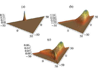
Figure 1: Plot of the evolution of an incident wave packet (a) after passing through the origin with $U=0$ in (b) and $U=2$ in (c). Note the strong scattering at an angle $\theta=-\pi/4$.

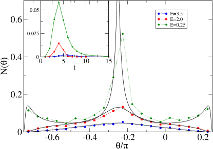
Figure 2: Plot of the number of particles scattered into a given direction for incident wave packets with different energies and $U=2$. The bold lines show the results from scattering theory estimated using $|f(\theta)|^{2}$ and the incident particle density at the origin (inset). Inset shows $|\Psi_{inc}({\bf 0},t)|^{2}$.

For the two-particle case it is more useful to study wave packets. We now consider the time evolution of wave packets and see how well the predictions of the scattering theory hold. The scattering states given by Eq. (3) are the full set of allowed two-particle energy eigenstates (for $U>\pi$ one gets an additional bound state sen ). These can be generated by a unitary time evolution of the unperturbed states which form a complete set. Hence these states also form a complete set, and any two-particle wave function can be expanded using this basis. Thus the time evolution of an initial wave packet $\Psi({\bf x},t=0)$ is given by

$$\Psi({\bf x},t)=\frac{1}{(2\pi)^{2}}\int_{-\pi}^{\pi}dq_{1}\int_{-\pi}^{q_{1}}dq_{2}~{}a({\bf q})\psi_{\bf q}({\bf x})~{}e^{-iE_{\bf q}t},$$

$${\rm where}~{}~{}a({\bf q})=\sum_{x_{1}>x_{2}}\Psi({\bf x},t=0)~{}\psi^{*}_{\bf q}({\bf x}).$$ (10)

The time evolution can be studied quite accurately because of our knowledge of the exact basis states. In evaluating the basis states, for small $(x_{1},x_{2})\lesssim 15$, we evaluate the Green’s functions $g^{+}_{E_{\bf k}}({\bf x})$ exactly using recursion relations morita71 relating these to $g_{E_{\bf k}}^{+}(0,0)$ and $g_{E_{\bf k}}^{+}(1,1)$. For larger $(x_{1},x_{2})$ we use the asymptotic forms which are quite accurate. We find that in our computations the normalization of the wave function is preserved to within $0.5\%$. In Fig. 1 we show the typical time-evolution of a wave packet with initial position and momentum localized at ${\bf x}=(-3.922,-5.0)$ and ${\bf q}=(2.554,0.785)$ respectively and with widths $\delta x\approx\delta q\approx 1$  and $E\approx 0.25$. These initial conditions have been chosen so that the two particles reach the site ${\bf 0}$ at roughly the same time; this maximizes their interaction. The initial wave packet shown in Fig. 1 ($a$) evolves at time $t=20$ to ($b$) for $U=0$ and to ($c$) for $U=2$. For the scattered wave function in Fig. 1 (c) we can count the number of particles scattered into a given direction. This is plotted in Fig. 2 for incident wave packets with different energies. We also compare this with the scattering theory prediction by plotting $|f(\theta)|^{2}$ multiplied by the time-integrated incident two-particle density at the origin. The comparison can be seen to be very good.

Transport calculation: We will now turn our attention to quantities of interest in transport calculations. The current density is given by the expectation value of the operator $j_{x}=-i(c_{x}^{\dagger}c_{x+1}-h.c.)$ in the scattering state $|\psi_{\bf k}\rangle=|\phi_{\bf k}\rangle+|S_{\bf k}\rangle$. The current in the incident state is given by $\langle\phi_{\bf k}|j_{x}|\phi_{\bf k}\rangle=2[\sin(k_{1})+\sin(k_{2})]{\cal N}$, where ${\cal{N}}$ is the total number of sites in the entire system. The change in current due to scattering, $\delta j(k_{1},k_{2})=\langle\psi_{\bf k}|j_{x}|\psi_{\bf k}\rangle-\langle\phi_{\bf k}|j_{x}|\phi_{\bf k}\rangle$, gets contributions from two parts, namely, $j_{S}=\langle S_{\bf k}|j_{x}|S_{\bf k}\rangle$ and $j_{C}=\langle S_{\bf k}|j_{x}|\phi_{\bf k}\rangle+\langle\phi_{\bf k}|j_{x}|S_{\bf k}\rangle$, and is of order $1$, i.e., it is a factor of $\cal N$ smaller than the current in the incident state aharony2 . We find that

$$\delta j(k_{1},k_{2})~{}=~{}\frac{2|\phi_{\bf k}({\bf 0})|^{2}Im[K_{E_{\bf k}}({\bf 0})]}{|1/U-K_{E_{\bf k}}({\bf 0})|^{2}}~{}[sgn(k_{1})+sgn(k_{2})],$$ (11)

where $sgn(k)\equiv|k|/k$.

$N$-particle scattering state and change in the Landauer current: We now consider the problem of calculating the current in a situation where the interacting region is connected to left and right leads which are at zero temperature and chemical potentials $\mu_{L}$ and $\mu_{R}$ respectively. In that case we have to consider an initial state with $N_{L}$ electrons in positive momentum states filling $1$-particle energy levels up to $\mu_{L}$ and $N_{R}$ electrons in negative momentum states filling levels up to $\mu_{R}$. Let $N=N_{L}+N_{R}$ and let us denote this $N$-particle incident wave by $|\phi^{(N)}\rangle=|{\bf k}^{(N)}\rangle$, where ${\bf k}^{(N)}=\{k_{1}k_{2}...k_{N}\}$. One then needs to find the corresponding scattering state and compute the particle current. An exact solution for the $N$-particle scattering state looks difficult. We will therefore restrict ourselves to an approximation in which only two-particle scattering is taken into account. Within this approximation, the scattered wave is given by $|\psi_{{\bf k}_{N}}\rangle=|\phi_{{\bf k}_{N}}\rangle+|S_{{\bf k}_{N}}\rangle$, where the transition amplitude to a wave vector ${\bf q}_{N}=\{q_{1}q_{2}...q_{N}\}$ is given by

$$\langle{\bf q}_{N}|S_{{\bf k}_{N}}\rangle = \sum_{{\bf q}_{2}{\bf k}_{2}}(-1)^{P+P^{\prime}}\langle{\bf q}_{2}|S_{{\bf k}_{2}}\rangle\langle{\bf q}^{\prime}_{N-2}{|{\bf k}^{\prime}_{N-2}}\rangle,$$

$${\rm with}~{}\langle{\bf q}_{2}|S_{{\bf k}_{2}}\rangle = \frac{\phi_{{\bf q}_{2}}^{*}({\bf 0})\phi_{{\bf k}_{2}}({\bf 0})}{(1/U-K_{E_{{\bf k}_{2}}}({{\bf 0}}))(E_{{\bf k}_{2}}-E_{{\bf q}_{2}}+i\epsilon)}.$$ (12)

Here ${\bf q}_{2}$ (${\bf k}_{2}$) denotes a pair of momenta chosen from the set ${\bf q}_{N}$ (${\bf k}_{N}$), and ${\bf q}^{\prime}$ (${\bf k}^{\prime}$) denotes the remaining $N-2$ momenta. $P$ ($P^{\prime}$) are the appropriate number of permutations. Using Eq. (12), we can calculate the current expectation value for the state $|\psi_{{\bf k}_{N}}\rangle$ to order $U^{2}$. (At order $U^{2}$, there are also contributions to the current from three- and four-particle scattering, but we will ignore those here). The current in the incident state $|\phi_{{\bf k}_{N}}\rangle$ is given by $\langle\phi|j_{x}|\phi\rangle=2[\sum_{j=1}^{N}\sin(k_{j})]{\cal N}^{N-1}$. The correct normalization is obtained by dividing by a factor ${\cal{N}}^{N}$ which then gives in the continuum limit: $j_{inc}=[\int_{0}^{k_{L}}dk~{}2\sin(k)-\int_{0}^{k_{R}}dk~{}2\sin(k)]/(2\pi)=(\mu_{L}-\mu_{R})/(2\pi)$, where $k_{L,R}=\cos^{-1}(-\mu_{L,R}/2)$, and we have used $dk=dE/|dE/dk|=dE/|2\sin(k)|$. Inserting factors of $\hbar$ and $e$, this gives the expected Landauer current $I=(e/h)(\mu_{L}-\mu_{R})$ and Landauer conductance $G=e^{2}/h$. The change in the Landauer current due to two-particle scattering is given by a sum of two-particle currents from all possible momentum pairs: $\delta j_{N}=(1/2)\sum_{r,s}\delta j(k_{r},k_{s})~{}{\cal{N}}^{N-2}$ which, with the same normalization as used earlier, gives

$$\delta j_{N}~{}=~{}\frac{1}{2(2\pi)^{2}}\int\int dk_{1}dk_{2}~{}\delta j(k_{1},k_{2}),$$ (13)

where the integrations are over the full range of allowed momenta $[-\pi,\pi]$, and $\delta j(k_{1},k_{2})$ is given by Eq. (11) [expanded to order $U^{2}$]. Using the fact that $\delta j(k_{1},k_{2})$ vanishes whenever $k_{1},k_{2}$ have opposite signs and converting Eq. (13) to energy integrals, we find the following correction to the Landauer current,

$$\delta j_{N} = [\int_{-2}^{\mu_{R}}dE_{k_{1}}\int_{\mu_{R}}^{\mu_{L}}dE_{k_{2}}+\frac{1}{2}\int_{\mu_{R}}^{\mu_{L}}dE_{k_{1}}\int_{\mu_{R}}^{\mu_{L}}dE_{k_{2}}]$$

$$\times \rho(E_{k_{1}})\rho(E_{k_{2}})~{}U^{2}4|\phi_{k_{1},k_{2}}({\bf 0})|^{2}~{}Im[K_{E_{k_{1},k_{2}}}({\bf 0})],$$

where $\rho(E)=1/(2\pi\sqrt{4-E^{2}})$ is the density of states. The quantity in Eq. (LABEL:curr) is negative because $Im[K_{E_{{\bf k}}}({\bf 0})]<0$ for all values of ${\bf k}$. In the zero bias limit $\mu_{L}\to\mu_{R}$, Eq. (LABEL:curr) vanishes as $U^{2}(\mu_{L}-\mu_{R})$ due to the contribution coming from the first set of integrals; thus $G$ is less than $e^{2}/h$ by a term of order $U^{2}$.

Finally, let us briefly discuss the case of spin-1/2 electrons. We consider the Hamiltonian $H=-\sum_{x=-\infty}^{\infty}\sum_{\sigma=\uparrow,\downarrow}~{}(c_{x,\sigma}^{\dagger}c_{x+1,\sigma}+h.c.)+Un_{0\uparrow}n_{0\downarrow}$. The interaction at the site 0 can cause scattering between two electrons in the singlet channel but not in the triplet channel. The scattering of two electrons in the singlet channel can be studied exactly using the Lippman-Schwinger formalism just as in Eqs. (2-3), except that the wave function for the state $|\phi_{{\bf k}}\rangle\equiv|k_{1},\uparrow;k_{2},\downarrow\rangle=-|k_{2},\downarrow;k_{1},\uparrow\rangle$ is now given by $\phi_{{\bf k}}({\bf x})=e^{i(k_{1}x_{1}+k_{2}x_{2})}$, and the Green’s function is given by $K_{E_{\bf k}}({\bf x})=[1/(2\pi)^{2}]\int_{-\pi}^{\pi}\int_{-\pi}^{\pi}{dq_{1}dq_{2}}{e^{i{\bf q}\cdot{\bf x}}}/(~{}E_{\bf k}-E_{\bf q}+i\epsilon)$. Finally, we can argue as in the spinless case, that in the presence of a Fermi sea, the scattering reduces the Landauer conductance by a term of order $U^{2}$.

Discussion: We have shown how the Lippman-Schwinger formalism can be used to obtain exact results for two particles scattering from an interacting region. This method can be applied to other cases, such as the two-wire system studied in Refs. goorden07 , the case of spin-$1/2$ electrons as mentioned above and the case with interactions on more than one bond. We have demonstrated how scattering theory can be used to understand numerical results for a two-particle wave packet moving through the interacting region. Finally, we have considered the problem of many-particle transport across the interacting region; we find that two-particle scattering reduces the zero-temperature Landauer conductance by a term of order $U^{2}$. This calculation is nontrivial since it considers many-particle states and is a fully nonequilibrium treatment. We expect the two-particle scattering approximation to be valid at low densities $k_{L,R}/\pi<<1$ rech since the $3$-particle correction given by $\int\int\int dk_{1}dk_{2}dk_{3}\delta j(k_{1},k_{2},k_{3})$ would be smaller by a factor of order $k_{L,R}/\pi$. In this paper we have considered the simplest case with interactions on a single bond and no impurities. For interactions on more than one bond, the form of the two-particle $S$-matrix would change but the qualitative conclusions remain the same sen . In the presence of impurities however, a term of $O(U)$ appears in the correction to $G$ and this could lead to an enhancement of $G$, depending on the sign of $U$. More generally, interactions can lead to dephasing and suppression of weak localization thereby increasing $G$ whitney .

We thank Natan Andrei, Markus Büttiker, Leonid Levitov, and Sumathi Rao for stimulating discussions.

References

(1)
(2) D. C. Ralph and R. A. Buhrman, Phys. Rev. Lett. 72, 3401
(1994); D. Goldhaber-Gordon et al., Nature 391, 156 (1998); W. G.
van der Wiel et al., Science 289, 2105 (2000); R. M. Potok et al., Nature 446, 167 (2007); R. Leturcq et al., Phys. Rev.
Lett. 95, 126603 (2005).
(3) P. Mehta and N. Andrei, Phys. Rev. Lett. 96, 216802 (2006).
(4) C. Caroli et al., J. Phys. C 4, 916 (1971).
(5) A. Dhar and D. Sen, Phys. Rev. B 73, 085119 (2006).
(6) T. N. Todorov, G. A. D. Briggs, and A. P. Sutton, J. Phys.:
Condens. Matter 5, 2389 (1993).
(7) N. S. Wingreen and Y. Meir, Phys. Rev. B 49, 11040
(1994); Y. Meir, N. S. Wingreen, and P. A. Lee, Phys. Rev. Lett. 70,
2601 (1993).
(8) A. V. Lebedev, G. B. Lesovik, and G. Blatter, Phys. Rev. Lett.
100, 226805 (2008).
(9) M. C. Goorden and M. Büttiker, Phys. Rev. B 77,
205323 (2008).
(10) A. Aharony, O. Entin-Wohlman, and Y. Imry, Phys. Rev. B
61, 5452 (2000).
(11) O. Entin-Wohlman et al., Europhys. Lett. 50, 354
(2000).
(12) M. C. Goorden and M. Büttiker, Phys. Rev. Lett. 99,
146801 (2007).
(13) J.-T. Shen and S. Fan, Phys. Rev. Lett. 98, 153003 (2007).
(14) D. Sen and A. Dhar, in preparation.
(15) E. N. Economou, Green’s Functions in Quantum Physics
(3rd edition, Springer, New York, 2006).
(16) T. Morita, J. Math. Phys. 12, 1744 (1971).
(17) J. Rech and K. A. Matveev, Phys. Rev. Lett. 100, 066407
(2008).
(18) R. S. Whitney, P. Jacquod, and C. Petitjean, Phys. Rev. B 77, 045315 (2008).