Java Application that Outputs
Quantum Circuit for Some
NAND Formula Evaluators

Abstract

This paper introduces QuanFruit v1.1, a Java application available for free. (Source code included in the distribution.) Recently, Farhi-Goldstone-Gutmann (FGG) wrote a paper arXiv:quant-ph/0702144 that proposes a quantum algorithm for evaluating NAND formulas. QuanFruit outputs a quantum circuit for the FFG algorithm.

1 Introduction

This paper introduces QuanFruit v1.1, a Java application available[1] for free. (Source code included in the distribution.) Recently, Farhi-Goldstone-Gutmann (FGG) wrote a paper[2] that proposes a quantum algorithm for evaluating NAND formulas. QuanFruit outputs a quantum circuit for the FFG algorithm.

We say a unitary operator acting on a set of qubits has been compiled if it has been expressed as a SEO (sequence of elementary operations, like CNOTs and single-qubit operations). SEO’s are often represented as quantum circuits.

There exist software (quantum compilers) like Qubiter[3] for compiling arbitrary unitary operators (operators that have no a priori known structure). QuanFruit is a special purpose quantum compiler. It is special purpose in the sense that it can only compile unitary operators that have a very definite, special structure.

The QuanFruit application is part of a suite of Java applications called QuanSuite. QuanSuite applications are all based on a common class library called QWalk. Each QuanSuite application compiles a different kind of quantum evolution operator. The applications output a quantum circuit that equals the input evolution operator. We have introduced 6 other QuanSuite applications in 2 earlier papers. Ref.[4] introduced QuanTree and QuanLin. Ref.[5] introduced QuanFou, QuanGlue, QuanOracle, and QuanShi. QuanFruit calls methods from these 6 previous applications, so it may be viewed as a composite of them.

Before reading this paper, the reader should read Refs.[4] and [5]. Many explanations in Refs.[4] and [5] still apply to this paper. Rather than repeating such explanations in this paper, the reader will be frequently referred to Refs.[4] and [5].

The goal of all QuanSuite applications, including QuanFruit, is to compile an input evolution operator $U$. $U$ can be specified either directly (e.g. in QuanFou, QuanShi), or by giving a Hamiltonian $H$ such that $U=e^{iH}$ (e.g. in QuanGlue and QuanOracle).

The standard definition of the evolution operator in Quantum Mechanics is $U=e^{-itH}$, where $t$ is time and $H$ is a Hamiltonian. Throughout this paper, we will set $t=-1$ so $U=e^{iH}$. If $H$ is proportional to a coupling constant $g$, reference to time can be restored easily by replacing the symbol $g$ by $-tg$, and the symbol $H$ by $-tH$.

2 Input Evolution Operator

The input evolution operator for QuanFruit is $U_{fruit}=e^{iH_{fruit}}$, where

$$H_{fruit}=\left[\begin{array}[]{c|c|c|c|c|c|c}\lx@intercol\hfil\hfil\lx@intercol\vrule\lx@intercol&h^{\dagger}_{glue}&&\\ \cline{5-7}\cr\lx@intercol\hfil\hfil\lx@intercol\vrule\lx@intercol&&&\\ \cline{5-7}\cr\lx@intercol\hfil\hfil\lx@intercol\vrule\lx@intercol&&&\\ \cline{5-7}\cr\lx@intercol\hfil{\raisebox{17.22217pt}[0.0pt]{$H_{line}$}}\hfil\lx@intercol\vrule\lx@intercol&&&\\ \hline\cr h_{glue}&&&&\lx@intercol\hfil\hfil\lx@intercol\vrule\lx@intercol&\\ \cline{1-4}\cr\cline{7-7}\cr&&&&\lx@intercol\hfil{\raisebox{4.30554pt}[0.0pt]{$H_{tree}$}}\hfil\lx@intercol\vrule\lx@intercol&h_{ora}^{\dagger}\\ \hline\cr&&&&&h_{ora}&\end{array}\right]\;.$$ (1)

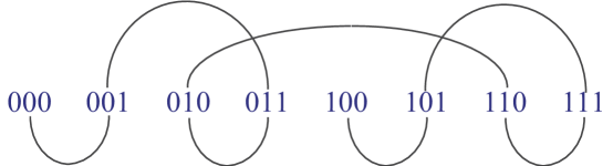
Figure 1: Line (open string) with 8 nodes

$H_{line}\in{\mathbb{R}}^{N_{S,line}\times N_{S,line}}$ where $N_{S,line}=2^{N_{B,line}}$ for some positive integer $N_{B,line}$. $H_{line}$ is proportional to the incidence matrix for a line graph, where the edges of the graph connect states that are consecutive in a Gray order. For example, for $N_{B,line}=3$, the graph of Fig.1 yields:

$$H_{line}=g\begin{array}[]{c|c|c|c|c|c|c|c|c|}&{\scriptscriptstyle 000}&{\scriptscriptstyle 001}&{\scriptscriptstyle 010}&{\scriptscriptstyle 011}&{\scriptscriptstyle 100}&{\scriptscriptstyle 101}&{\scriptscriptstyle 110}&{\scriptscriptstyle 111}\\ \hline\cr{\scriptscriptstyle 000}&0&1&&&&&&\\ \hline\cr{\scriptscriptstyle 001}&1&0&&1&&&&\\ \hline\cr{\scriptscriptstyle 010}&&&0&1&&&1&\\ \hline\cr{\scriptscriptstyle 011}&&1&1&0&&&&\\ \hline\cr{\scriptscriptstyle 100}&&&&&0&1&&\\ \hline\cr{\scriptscriptstyle 101}&&&&&1&0&&1\\ \hline\cr{\scriptscriptstyle 110}&&&1&&&&0&1\\ \hline\cr{\scriptscriptstyle 111}&&&&&&1&1&0\\ \hline\cr\end{array}\;,$$ (2)

where $g$ is a real number that we will call the coupling constant.

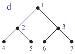
Figure 2: Binary tree with 8 nodes

$H_{tree}\in{\mathbb{R}}^{N_{S,tree}\times N_{S,tree}}$ where $N_{S,tree}=2^{N_{B,tree}}$ for some positive integer $N_{B,tree}$. $H_{tree}$ is proportional to the incidence matrix for a balanced-binary tree graph. For example, for $N_{B,tree}=3$, the graph of Fig.2 yields:

$$H_{tree}=g\begin{array}[]{c|c|c|c|c|c|c|c|c|}&{\scriptscriptstyle d}&{\scriptscriptstyle 1}&{\scriptscriptstyle 2}&{\scriptscriptstyle 3}&{\scriptscriptstyle 4}&{\scriptscriptstyle 5}&{\scriptscriptstyle 6}&{\scriptscriptstyle 7}\\ \hline\cr{\scriptscriptstyle d}&&&&&&&&\\ \hline\cr{\scriptscriptstyle 1}&&&1&1&&&&\\ \hline\cr{\scriptscriptstyle 2}&&1&&&1&1&&\\ \hline\cr{\scriptscriptstyle 3}&&1&&&&&1&1\\ \hline\cr{\scriptscriptstyle 4}&&&1&&&&&\\ \hline\cr{\scriptscriptstyle 5}&&&1&&&&&\\ \hline\cr{\scriptscriptstyle 6}&&&&1&&&&\\ \hline\cr{\scriptscriptstyle 7}&&&&1&&&&\\ \hline\cr\end{array}\;,$$ (3)

where $g$ is the same coupling constant as before.

$h_{glue}\in{\mathbb{R}}^{1\times 1}$. In fact,

$$h_{glue}=g|N_{S,line}+1\rangle\langle d|\;.$$ (4)

Here $|N_{S,line}+1\rangle$ labels the god state of the tree, the one with children but no parents.( $N_{S,line}$ labels the dud node) We will call $d\in Z_{0,N_{S,line}-1}$ the line door. If $d=0$, then the tree is connected to a tail of states. For $N_{B,line}=3$, from Fig.1, if $d=2$, then the tree is connected to the midpoint of the line of states (“runway”).

The number of leaves in the tree is half the number of nodes in the tree: $N_{S,lvs}=\frac{N_{S,tree}}{2}$. Also, $N_{S,lvs}=2^{N_{B,lvs}}$ for some positive integer $N_{B,lvs}$. $h_{oracle}\in{\mathbb{R}}^{N_{S,lvs}\times N_{S,lvs}}$. In fact,

$$h_{oracle}=g\left[\begin{array}[]{cccc}x_{0}&&&\\ &x_{1}&&\\ &&\ddots&\\ &&&x_{{N_{lvs}}-1}\end{array}\right]\;,$$ (5)

where $x_{k}\in Bool$ are the inputs to the NAND formula.

The dimension of the matrix $H_{fruit}$ is not generally a power of two. To represent it as a quantum circuit, we need to extend it to $diag(H_{fruit},0)\in{\mathbb{R}}^{{N_{S}}\times{N_{S}}}$, where

$${N_{S}}=2^{N_{B}}\;,\;\;{N_{B}}=\min\{N:N_{S,line}+\frac{3}{2}N_{S,tree}\leq 2^{N}\}\;.$$ (6)

Define

$$H_{glue}=h_{glue}+h_{glue}^{\dagger}\;,\;\;H_{ora}=h_{ora}+h_{ora}^{\dagger}\;.$$ (7)

(This last equation is fine as an operator statement, but as a matrix statement, $h_{glue}$ and $h_{glue}^{\dagger}$ must be “padded” with zeros to make the equation true. By “padding a matrix with zeros”, we mean embedding it in a larger matrix, the new entries being zeros.)

One can split $H_{fruit}$ into two parts, which we call the bulk Hamiltonian $H_{bulk}$ and the boundary corrections Hamiltonian $H_{corr}$:

$$H_{fruit}=H_{bulk}+H_{corr}\;,$$ (8)

where

$$H_{bulk}=H_{line}+H_{tree}\;\;\;,\;\;\;H_{corr}=H_{glue}+H_{ora}\;.$$ (9)

(Again, this last equation requires zero padding if considered a matrix equation.) Note that $[H_{line},H_{tree}]=0$ and $[H_{glue},H_{ora}]=0$.

For $r=1,2,3,\ldots$, if $U=L_{r}(g)+{\cal O}(g^{r+1})$, we say $L_{r}(g)$ approximates (or is an approximant) of order $r$ for $U$.

Given an approximant $L_{r}(g)+{\cal O}(g^{r+1})$ of $U$, and some ${N_{T}}=1,2,3\,\ldots$, one can approximate $U$ by $\left(L_{r}(\frac{g}{{N_{T}}})\right)^{N_{T}}+{\cal O}(\frac{g^{r+1}}{{N_{T}}^{r}})$. We will refer to this as Trotter’s trick, and to ${N_{T}}$ as the number of trots.

For $N_{T,line}=1$, QuanFruit approximates $e^{iH_{line}}$ with a Suzuki approximant of order $r_{line}=2,4,6,\ldots$ that is derived in Ref.[6]. QuanFruit also applies the Trotter trick with $N_{T,line}>1$ trots to the $N_{T,line}=1$ approximant of $e^{iH_{line}}$.

For $N_{T,tree}=1$, QuanFruit always approximates $e^{iH_{tree}}$ with an approximant of order 3, that is derived in Ref.[6]. QuanFruit also applies the Trotter trick with $N_{T,tree}>1$ trots to the $N_{T,tree}=1$ approximant of $e^{iH_{tree}}$.

Ref.[6] gives exact (to numerical precision) compilations of the glue and oracle parts of $U_{fruit}$. QuanFruit uses these compilations, so the Order of the Suzuki (or other) Approximant and the Number of Trots do not arise in QuanFruit, for either the glue or the oracle.

For $N_{T,meta}=1$, QuanFruit also approximates $e^{iH_{fruit}}$ with a Suzuki approximant of order $r_{meta}=2,4,6,\ldots$. Recall that $S_{2}(t)=e^{A\frac{t}{2}}e^{Bt}e^{A\frac{t}{2}}$ for $t\in{\mathbb{R}}$ is the second order Suzuki approximant, and higher order ones are defined recursively from this one. Thus, all Suzuki approximants are specified by giving two functions of $t$, $e^{At}$ and $e^{Bt}$. To get a “meta” Suzuki approximant, we set $e^{At}=e^{i(H_{bulk})_{g\rightarrow t}}$ and $e^{Bt}=e^{i(H_{corr})_{g\rightarrow t}}$. QuanFruit also applies the Trotter trick with $N_{T,meta}>1$ trots to the $N_{T,meta}=1$ approximant of $e^{iH_{fruit}}$.

3 The Control Panel

Fig.3 shows the Control Panel for QuanFruit. This is the main and only window of the application. This window is open if and only if the application is running.

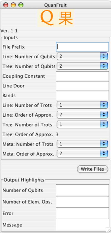
Figure 3: Control Panel of QuanFruit

The Control Panel allows you to enter the following inputs:

File Prefix:

Prefix to the 3 output files that are written when you press the Write Files button. For example, if you insert test in this text field, the following 3 files will be written:

• test_qfru_log.txt

• test_qfru_eng.txt

• test_qfru_pic.txt

Line: Number of Qubits:

The parameter $N_{B,line}$ defined above.

Tree: Number of Qubits:

The parameter $N_{B,tree}$ defined above.

Coupling Constant:

The parameter $g\in{\mathbb{R}}$ defined above.

Line Door:

The parameter $d\in Z_{0,N_{S,line}-1}$ defined above.

Bands:

You must enter here an even number of integers separated by any non-integer, non-white space symbols. Say you enter $a_{1},b_{1},a_{2},b_{2},\ldots,a_{n},b_{n}$. If $x_{k}\in Bool$ for $k\in Z_{0,{N_{lvs}}-1}$ are as defined above, then $x_{k}=1$ iff $k\in Z_{a_{1},b_{1}}\cup Z_{a_{2},b_{2}}\ldots\cup Z_{a_{n},b_{n}}$. Each set $Z_{a_{k},b_{k}}$ is a “band”. If $a_{k}=b_{k}$, the band has a single element. QuanFruit checks that $0\leq a_{0}$, $b_{n}\leq({N_{lvs}}-1)$, and $b_{k}-a_{k}\geq 0$ for all $k$. It also checks that $a_{k+1}-b_{k}\geq 2$. (If $a_{k+1}-b_{k}=1$, bands $k+1$ and $k$ can be merged. If $a_{k+1}-b_{k}=0,-1,-2,\ldots$, bands $k+1$ and $k$ overlap.)

Line: Number of Trots:

The parameter $N_{T,line}$ defined above.

Line: Order of Approximant:

The parameter $r_{line}$ defined above.

Tree: Number of Trots:

The parameter $N_{T,tree}$ defined above.

Tree: Order of Approximant:

This parameter is always 3.

Meta: Number of Trots:

The parameter $N_{T,meta}$ defined above.

Meta: Order of Approximant:

The parameter $r_{meta}$ defined above.

The Control Panel displays the following outputs:

Number of Qubits:

The parameter ${N_{B}}$ defined by Eq.(6).

Number of Elementary Operations:

The number of elementary operations in the output quantum circuit. If there are no LOOPs, this is the number of lines in the English File, which equals the number of lines in the Picture File. When there are LOOPs, the “LOOP k REPS:${N_{T}}$” and “NEXT k” lines are not counted, whereas the lines between “LOOP k REPS:${N_{T}}$” and “NEXT k” are counted ${N_{T}}$ times.

Error:

The distance in the Frobenius norm between the input evolution operator and the output quantum circuit (i.e., the SEO given in the English File). For a nice review of matrix norms, see Ref.[7]. For any matrix $A\in{\mathbb{C}}^{n\times n}$, its Frobenius norm is defined as $\|A\|_{F}=\sqrt{\sum_{j,k}A_{j,k}A^{*}_{j,k}}$. Another common matrix norm is the 2-norm. The 2-norm $\|A\|_{2}$ of $A$ equals the largest singular value of $A$. The Frobenius and 2-norm of $A$ are related by[7]: $\|A\|_{2}\leq\|A\|_{F}\leq\sqrt{2}\|A\|_{2}$.

Message:

A message appears in this text field if you press Write Files with a bad input. The message tries to explain the mistake in the input.

4 Output Files

Pressing the Write Files button of the Control Panel of QuanFruit generates 3 files (Log, English, Picture). These files are analogous to their namesakes for QuanTree, QuanLin and other QuanSuite applications. Ref.[4] explains how to interpret them.

5 Behind the Scenes:
Code Innovations in QuanSuite, QWalk

The QuanSuite applications, based on the QWalk class library, exhibit some code innovations that you will find very helpful. Hopefully, these innovations will become commonplace in future quantum computer software.

• QWalk class library does most of the work in all QuanSuite applications: Look in the source folder for any of the QuanSuite applications. You’ll find that it contains only 3 or 4 classes. Most of the classes are in the source folder for QWalk. That’s because most of the work is done by the QWalk class library, which is independent of the QuanSuite application.

• Reusability of SEO writers: Look at the class FruitSEO_writer in the source folder for QuanFruit. You’ll find that FruitSEO_writer utilizes the methods GlueSEO_writer(), OracleSEO_writer(), TreeSEO_writer(), LineSEO_writer(), and ShiftSEO_writer(). Thus, FruitSEO_writer delegates its SEO writing to methods from the QuanSuite applications: QuanGlue, QuanOracle, QuanTree, QuanLin and QuanShi. In fact, QuanFruit can be viewed as a composite of these simpler QuanSuite applications. This reusability of SEO writers is made possible by the novel technique described in Appendix A.

• Nested Loops: The English and Picture files of QuanSuite applications can have LOOPs within LOOPs. This makes the English and Picture files shorter, without loss of information. However, if you want to multiply out all the operations in an English file (this is what the class SEO_reader in QWalk does), then having nested loops makes this task more difficult. SEO_reader of QWalk is sophisticated enough to understand nested loops.

• Painless object oriented implementation of Suzuki approximants and Trotter’s trick: Higher order Suzuki approximants can be implemented painlessly by using the classes: QWalk/src/SuzFunctions and QWalk/src/SuzWriter. See the class QuanLin/src/LineSEO_writer for an example of how it’s done. Essentially, all you have to do is to override the two abstract methods in QWalk/src/SuzFunctions.

  Trotter’s trick can also be easily implemented in a QuanSuite application, by using LOOP and NEXT lines in the English file. See the write() method of QuanLin/src/LineSEO_writer for an example.

Appendix A Appendix: $P_{0}$ Padding and State Shifting

Suppose we know how to compile $e^{iH}$. Is it possible to use this compilation to compile $e^{i\;\;diag(Z,H,Z^{\prime})}$, where $Z$ and $Z^{\prime}$ are square matrices of zeros? The answer is yes, as we show next.

Suppose $\hat{N}_{S}>{N_{S}}$ where ${N_{S}}=2^{N_{B}}$ and $\hat{N}_{S}=2^{\hat{N}_{B}}$, for some positive integers ${N_{B}}$ and $\hat{N}_{B}$. Given a Hamiltonian $H$, define a zero padded version of it called $\hat{H}$:

$$\hat{H}_{\hat{N}_{S}\times\hat{N}_{S}} = \left[\begin{array}[]{c|c}H_{{N_{S}}\times{N_{S}}}&\\ \hline\cr&0_{(\hat{N}_{S}-{N_{S}})\times(\hat{N}_{S}-{N_{S}})}\end{array}\right]$$ (10c)

$$= {\overline{n}}(\hat{N}_{B}-1)\otimes{\overline{n}}(\hat{N}_{B}-2)\otimes\cdots\otimes{\overline{n}}({N_{B}}+1)\otimes{\overline{n}}({N_{B}})\otimes H_{{N_{S}}\times{N_{S}}}\;.$$ (10d)

As usual, ${\overline{n}}()=P_{0}()$. We will say that $H$ has been padded with $P_{0}$’s to obtain $\hat{H}$. Now let $U_{shift}^{(k)}$ be the unitary operation that shifts state $|x\rangle$ to $|(x+k)\mod\hat{N}_{S}\rangle$, with $x,k\in Z_{0,\hat{N}_{S}-1}$. The application QuanShi gives a compilation of $U_{shift}^{(k)}$. Using $U_{shift}^{(k)}$, one can define a matrix $\hat{H}^{(k)}$ from $\hat{H}$ as follows:

$$(\hat{H}^{(k)})_{\hat{N}_{S}\times\hat{N}_{S}} = \left[\begin{array}[]{c|c|c}0_{k\times k}&&\\ \hline\cr&H_{{N_{S}}\times{N_{S}}}&\\ \hline\cr&&0_{(\hat{N}_{S}-{N_{S}}-k)\times(\hat{N}_{S}-{N_{S}}-k)}\end{array}\right]$$ (11d)

$$= (U_{shift}^{(k)})^{\dagger}\hat{H}_{\hat{N}_{S}\times\hat{N}_{S}}U_{shift}^{(k)}\;.$$ (11e)

It is now readily apparent that a SEO for $e^{i\;\;diag(Z,H,Z^{\prime})}$ can be obtained from a SEO for $e^{iH}$ by $P_{0}$ padding $H$ and then state shifting it with $U_{shift}^{(k)}$.

The compilations of $e^{iH_{line}}$ (given in QuanLin), $e^{iH_{tree}}$ (given in QuanTree) and $e^{iH_{ora}}$ (given in QuanOracle), are all utilized by QuanFruit via this $P_{0}$ padding/state-shifting method.

References

- [1] QuanFruit software available at www.ar-tiste.com/QuanSuite.html
- [2] E. Farhi, J. Goldstone, S. Gutmann, “A Quantum Algorithm for the Hamiltonian NAND Tree”, arXiv:quant-ph/0702144
- [3] R.R. Tucci, “A Rudimentary Quantum Compiler(2cnd Ed.)”, arXiv:quant-ph/9902062 . Qubiter software available at www.ar-tiste.com/qubiter.html
- [4] R.R. Tucci, “QuanTree and QuanLin, Two Special Purpose Quantum Compilers”, arXiv:0712.3887
- [5] R.R. Tucci, “QuanFou, QuanGlue, QuanOracle and QuanShi, Four Special Purpose Quantum Compilers”, arXiv:0802.2367
- [6] R.R.Tucci, “How to Compile Some NAND Formula Evaluators”, arXiv:0706.0479
- [7] G.H. Golub and C.F. Van Loan, Matrix Computations, Third Edition (John Hopkins Univ. Press, 1996).