QuanFou, QuanGlue, QuanOracle and QuanShi,
Four Special Purpose Quantum Compilers

Abstract

This paper introduces QuanFou v1.1, QuanGlue v1.1, QuanOracle v1.1, QuanShi v1.1, four Java applications available for free. (Source code included in the distribution.) Each application compiles a different kind of input quantum evolution operator. The applications output a quantum circuit that equals the input evolution operator.

1 Introduction

This paper introduces QuanFou v1.1, QuanGlue v1.1, QuanOracle v1.1, QuanShi v1.1, four Java applications available[1] for free. (Source code included in the distribution.)

In a previous paper[2], we introduced the Java applications QuanTree and QuanLin. These two applications plus the four applications introduced in this paper, are part of a suite of Java applications called QuanSuite. QuanSuite applications all depend heavily on a common class library called QWalk. Each QuanSuite application compiles a different kind of input quantum evolution operator. The applications output a quantum circuit that equals the input evolution operator.

Before reading this paper, the reader should read Ref.[2]. Many explanations in Ref.[2] still apply to this paper. Rather than repeating such explanations in this paper, the reader will be frequently referred to Ref.[2].

The input evolution operator $U$ for a QuanSuite application can be specified either directly (e.g. in QuanFou, QuanShi), or by giving a Hamiltonian $H$ such that $U=e^{iH}$ (e.g. in QuanGlue and QuanOracle).

The standard definition of the evolution operator in Quantum Mechanics is $U=e^{-itH}$, where $t$ is time and $H$ is a Hamiltonian. Throughout this paper, we will set $t=-1$ so $U=e^{iH}$. If $H$ is proportional to a coupling constant $g$, reference to time can be restored easily by replacing the symbol $g$ by $-tg$, and the symbol $H$ by $-tH$.

2 QuanFou

The input evolution operator for QuanFou is $U_{DFT}$, the Discrete Fourier Transform matrix, defined by:

$$(U_{DFT})_{p,q}=\frac{1}{\sqrt{{N_{S}}}}\omega^{pq}\;\;{\rm where}\;\;\omega=e^{i\frac{2\pi}{{N_{S}}}}\;,$$ (1)

with $p,q\in Z_{0,{N_{S}}-1}$.

See Ref.[3] for a review of how to compile $U_{DFT}$ exactly.

Since we use an exact (to numerical precision) compilation of $U_{DFT}$, the Order of the Suzuki(or other) Approximant and the Number of Trots are two parameters which do not arise in QuanFou (unlike QuanTree and QuanLin).

Fig.1 shows the Control Panel for QuanFou. This is the main and only window of the application.

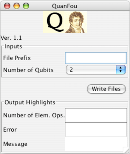
Figure 1: Control Panel of QuanFou

As to the input and output fields in the Control Panel for QuanFou, we’ve seen and explained these before in Ref.[2].

As to the output files (Log, English, Picture) generated when we press the Write Files button, we’ve seen and explained these before in Ref.[2]. For example, Figs.2, 3, 4 show an instance of these output files that was generated by QuanFou.

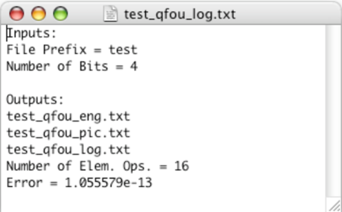
Figure 2: Log File generated by QuanFou

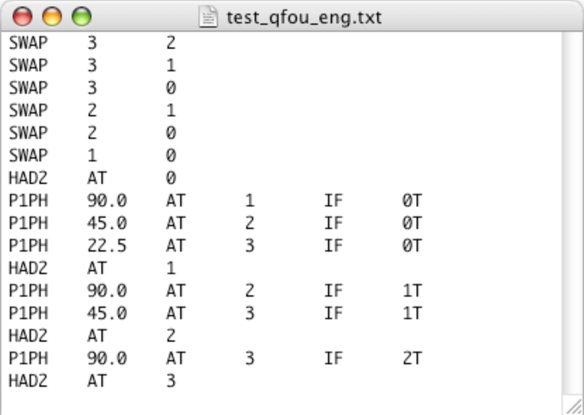
Figure 3: English File generated by QuanFou

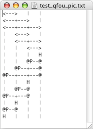
Figure 4: Picture File generated by QuanFou

3 QuanGlue

The input evolution operator for QuanGlue is $U_{glue}=e^{iH_{glue}}$, where:

$$H_{glue}=g(|r_{1}\rangle\langle r_{2}|+h.c.)\;,$$ (2)

for some $r_{1},r_{2}\in Z_{0,{N_{S}}-1}$.

Ref.[4] explains our method for compiling $U_{glue}$ exactly.

Since we use an exact (to numerical precision) compilation of $U_{glue}$, the Order of the Suzuki(or other) Approximant and the Number of Trots are two parameters which do not arise in QuanGlue (unlike QuanTree and QuanLin).

Fig.5 shows the Control Panel for QuanGlue. This is the main and only window of the application.

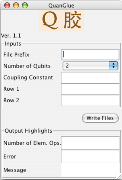
Figure 5: Control Panel of QuanGlue

As to the input and output fields in the Control Panel for QuanGlue, we’ve seen and explained these before in Ref.[2], except for the input fields Row 1 and Row 2.

Row 1, Row 2:

Row 1 = $r_{1}$ and Row 2 = $r_{2}$ or vice versa, where $r_{1},r_{2}$ are the parameters defined above, the two states being glued.

As to the output files (Log, English, Picture) generated when we press the Write Files button, we’ve seen and explained these before in Ref.[2].

4 QuanOracle

Consider a tree with $N_{S,tree}$ states, and ${N_{lvs}}=\frac{N_{S,tree}}{2}$ leaves, with leaf inputs $x_{k}\in Bool$ for $k\in Z_{0,{N_{lvs}}-1}$. The input evolution operator for QuanOracle is $U_{oracle}=e^{iH_{oracle}}$, where

$$H_{oracle} = g\left[\begin{array}[]{cccc|cccc}&&&&x_{0}&&&\\ &&&&&x_{1}&&\\ &&&&&&\ddots&\\ &&&&&&&x_{{N_{lvs}}-1}\\ \hline\cr x_{0}&&&&&&&\\ &x_{1}&&&&&&\\ &&\ddots&&&&&\\ &&&x_{{N_{lvs}}-1}&&&&\end{array}\right]\;.$$ (3i)

Ref.[4], in the appendix for “banded oracles”, explains our method for compiling $U_{oracle}$ exactly.

Since we use an exact (to numerical precision) compilation of $U_{oracle}$, the Order of the Suzuki(or other) Approximant and the Number of Trots are two parameters which do not arise in QuanOracle (unlike QuanTree and QuanLin).

Fig.6 shows the Control Panel for QuanOracle. This is the main and only window of the application.

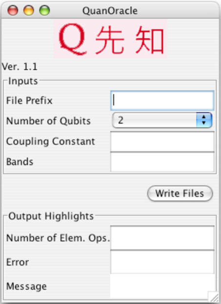
Figure 6: Control Panel of QuanOracle

As to the input and output fields in the Control Panel for QuanOracle, we’ve seen and explained these before in Ref.[2], except for the input field Bands.

Bands:

You must enter here an even number of integers separated by any non-integer, non-white space symbols. Say you enter $a_{1},b_{1},a_{2},b_{2},\ldots,a_{n},b_{n}$. If $x_{k}\in Bool$ for $k\in Z_{0,{N_{lvs}}-1}$ are as defined above, then $x_{k}=1$ iff $k\in Z_{a_{1},b_{1}}\cup Z_{a_{2},b_{2}}\ldots\cup Z_{a_{n},b_{n}}$. Each set $Z_{a_{k},b_{k}}$ is a “band”. If $a_{k}=b_{k}$, the band has a single element. QuanOracle checks that $0\leq a_{0}$, $b_{n}\leq({N_{lvs}}-1)$, and $b_{k}-a_{k}\geq 0$ for all $k$. It also checks that $a_{k+1}-b_{k}\geq 2$. (If $a_{k+1}-b_{k}=1$, bands $k+1$ and $k$ can be merged. If $a_{k+1}-b_{k}=0,-1,-2,\ldots$, bands $k+1$ and $k$ overlap.)

As to the output files (Log, English, Picture) generated when we press the Write Files button, we’ve seen and explained these before in Ref.[2].

5 QuanShi

The input evolution operator for QuanShi is the unitary operation $U_{shift}$ that takes:

$$|x\rangle\rightarrow|(x+t)\mod{N_{S}}\rangle\;,$$ (4)

where $x,t\in Z_{0,{N_{S}}-1}$, with ${N_{S}}=2^{N_{B}}$ for some positive integer ${N_{B}}$. We call $t$ the state shift.

$U_{shift}$ can be easily expressed in matrix form. For example, for ${N_{S}}=8$ and $t=3$,

$$U_{shift}=\begin{array}[]{c||c|c|c|c|c|c|c|c|}&{\scriptscriptstyle 0}&{\scriptscriptstyle 1}&{\scriptscriptstyle 2}&{\scriptscriptstyle t}&&&&\\ \hline\cr\hline\cr{\scriptscriptstyle 0}&&&&1&&&&\\ \hline\cr{\scriptscriptstyle 1}&&&&&1&&&\\ \hline\cr{\scriptscriptstyle 2}&&&&&&1&&\\ \hline\cr{\scriptscriptstyle\vdots}&&&&&&&1&\\ \hline\cr&&&&&&&&1\\ \hline\cr{\scriptscriptstyle{N_{S}}-t}&1&&&&&&&\\ \hline\cr&&1&&&&&&\\ \hline\cr{\scriptscriptstyle{N_{S}}-1}&&&1&&&&&\\ \hline\cr\end{array}\;.$$ (5)

Appendix A explains our method for compiling $U_{shift}$ exactly.

Since we use an exact (to numerical precision) compilation of $U_{shift}$, the Order of the Suzuki(or other) Approximant and the Number of Trots are two parameters which do not arise in QuanShi (unlike QuanTree and QuanLin).

Fig.7 shows the Control Panel for QuanShi. This is the main and only window of the application.

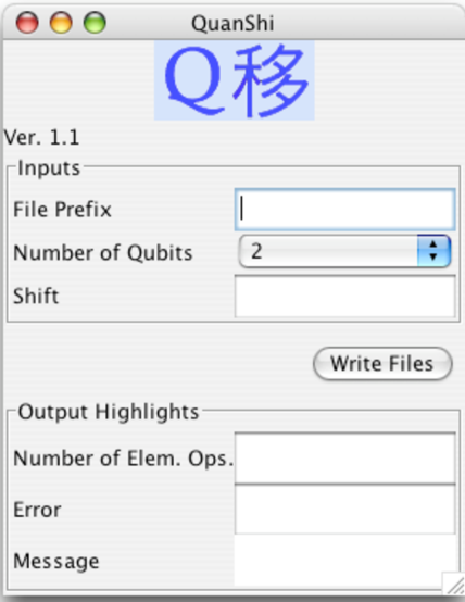
Figure 7: Control Panel of QuanShi

As to the input and output fields in the Control Panel for QuanShi, we’ve seen and explained these before in Ref.[2], except for the input field Shift.

Shift:

The parameter $t$ defined above. QuanShi allows $-{N_{S}}<t<{N_{S}}$ and interprets a shift by $-t$ as the inverse of a shift by $t$.

As to the output files (Log, English, Picture) generated when we press the Write Files button, we’ve seen and explained these before in Ref.[2].

Appendix A Appendix: How to Compile a State Shift

In this appendix, we will show how to compile the unitary operation $U_{shift}$ that takes

$$|x\rangle\rightarrow|(x+t)\mod{N_{S}}\rangle\;,$$ (6)

where $x,t\in Z_{0,{N_{S}}-1}$, with ${N_{S}}=2^{N_{B}}$ for some positive integer ${N_{B}}$. We call $t$ the state shift.

$U_{shift}$ can be easily expressed in matrix form. For example, for ${N_{S}}=8$ and $t=3$,

$$U_{shift}=\begin{array}[]{c||c|c|c|c|c|c|c|c|}&{\scriptscriptstyle 0}&{\scriptscriptstyle 1}&{\scriptscriptstyle 2}&{\scriptscriptstyle t}&&&&\\ \hline\cr\hline\cr{\scriptscriptstyle 0}&&&&1&&&&\\ \hline\cr{\scriptscriptstyle 1}&&&&&1&&&\\ \hline\cr{\scriptscriptstyle 2}&&&&&&1&&\\ \hline\cr{\scriptscriptstyle\vdots}&&&&&&&1&\\ \hline\cr&&&&&&&&1\\ \hline\cr{\scriptscriptstyle{N_{S}}-t}&1&&&&&&&\\ \hline\cr&&1&&&&&&\\ \hline\cr{\scriptscriptstyle{N_{S}}-1}&&&1&&&&&\\ \hline\cr\end{array}\;.$$ (7)

$U_{shift}$ is an example of a circulant matrix. Ref.[4] reviews the well known properties of circulant matrices. Circulant matrices have a particularly simple eigenvalue decomposition. Define

$$\omega=e^{-i\frac{2\pi}{{N_{S}}}}\;.$$ (8)

Then, according to Ref.[4],

$$U_{shift}=VDV^{\dagger}\;,$$ (9)

where

$$V_{p,q}=\frac{1}{\sqrt{{N_{S}}}}\omega^{pq}\;,$$ (10)

and

$$D=diag({\lambda}_{0},{\lambda}_{1},\ldots,{\lambda}_{{N_{S}}-1})\;\;{\rm with}\;\;{\lambda}_{m}=\omega^{mt}\;.$$ (11)

Note that $V^{\dagger}$ is the DFT matrix.

It follows that

$$D=\exp(-i\frac{2\pi}{{N_{S}}}tA)\;,$$ (12)

where

$$A=\left[\begin{array}[]{ccccc}0&&&&\\ &1&&&\\ &&2&&\\ &&&\ddots&\\ &&&&{N_{S}}-1\end{array}\right]=\sum_{\vec{m}\in Bool^{N_{B}}}mP_{\vec{m}}\;.$$ (13)

We are using $\vec{m}=(m_{{N_{B}}-1},\ldots,m_{2},m_{1},m_{0})$, and $m=dec(\vec{m})=2^{{N_{B}}-1}m_{{N_{B}}-1}+\cdots+2^{2}m_{2}+2m_{1}+m_{0}$.

Consider $A$ for ${N_{B}}=2$:

$$0P_{00}+1P_{01}+2P_{10}+3P_{11} = P_{01}+2P_{1.}+P_{11}$$ (14a)

$$= P_{.1}+2P_{1.}$$ (14b)

$$= n(0)+2n(1)\;.$$ (14c)

Now consider $A$ for ${N_{B}}=3$:

$$\sum_{\vec{m}\in Bool^{3}}(2^{2}m_{2}+2m_{1}+m_{0})P_{\vec{m}} = \sum_{\vec{m}\in Bool^{3}}(2^{2}m_{2}P_{\vec{m}})+2n(1)+n(0)$$ (15a)

$$= 2^{2}P_{1..}+2n(1)+n(0)$$ (15b)

$$= 2^{2}n(2)+2n(1)+n(0)\;.$$ (15c)

This result can be easily generalized using induction to an arbitrary number of qubits.

An exact compilation of $U_{shift}$ is now readily apparent from Eq.(9). The matrices $V$ and $V^{\dagger}$ are DFTs matrices so we know how to compile them. The diagonal matrix $D$ is also easy to compile. For example, for ${N_{B}}=3$,

$${{{{{{{{D=\exp\left(-i\frac{2\pi}{{N_{S}}}t[2^{2}n(2)+2n(1)+n(0)]\right)=\begin{array}[]{c}\lx@xy@svg{\hbox{&*+[F]{e^{i\phi n}} \ignorespaces\ignorespaces\ignorespaces\ignorespaces\ignorespaces{}\ignorespaces{\hbox{\lx@xy@droprule}}\ignorespaces{\hbox{\kern 0.0pt\raise 0.0pt\hbox{\hbox{\kern 0.0pt\raise 0.0pt\hbox{\lx@xy@tip{1}\lx@xy@tip{-1}}}}}}\ignorespaces{\hbox{\lx@xy@droprule}}{\hbox{\lx@xy@droprule}}\ignorespaces @{-} [0,-1]}&\ignorespaces\ignorespaces\ignorespaces\ignorespaces\ignorespaces{}\ignorespaces{\hbox{\lx@xy@droprule}}\ignorespaces{\hbox{\kern 0.0pt\raise 0.0pt\hbox{\hbox{\kern 0.0pt\raise 0.0pt\hbox{\lx@xy@tip{1}\lx@xy@tip{-1}}}}}}\ignorespaces{\hbox{\lx@xy@droprule}}{\hbox{\lx@xy@droprule}}\ignorespaces @{-} [0,-1]\\ &*+[F]{e^{i2\phi n}} \xy@@ix@{{\hbox{}}}}{-}}\ignorespaces\PATHlabelsextra@@@{-} [0,-1]&\xy@@ix@{{\hbox{}}}}{-}}\ignorespaces\PATHlabelsextra@@@{-} [0,-1]\\ &*+[F]{e^{i4\phi n}}\xy@@ix@{{\hbox{}}}}{-}}\ignorespaces\PATHlabelsextra@@@{-}[0,-1]&\xy@@ix@{{\hbox{}}}}{-}}\ignorespaces\PATHlabelsextra@@@{-}[0,-1]}\end{array}\;,$$ (16)

where $\phi=-\frac{2\pi}{{N_{S}}}t$.

References

- [1] QuanFou, QuanGlue, QuanOracle and QuanShi software available at www.ar-tiste.com/QuanSuite.html
- [2] R.R. Tucci, “QuanTree and QuanLin, Two Special Purpose Quantum Compilers”, arXiv:0712.3887
- [3] R.R.Tucci, “QC Paulinesia”, quant-ph/0407215
- [4] R.R.Tucci, “How to Compile Some NAND Formula Evaluators”, arXiv:0706.0479