Quantum Stirring in low dimensional devices

Abstract

A circulating current can be induced in the Fermi sea by displacing a scatterer, or more generally by integrating a quantum pump into a closed circuit. The induced current may have either the same or the opposite sense with respect to the “pushing” direction of the pump. We work out explicit expressions for the associated geometric conductance using the Kubo-Dirac monopoles picture, and illuminate the connection with the theory of adiabatic passage in multiple path geometry.

I Introduction

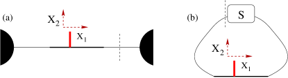
Figure 1: In the case of an open geometry the pumping device is connected between two unbiased reservoirs (panel (a)), while in the present study it is integrated into a ring (panel (b)). The induced current is measured through a section indicated by a dashed line. See the text for further details.

The question “how much charge is transported due to an adiabatic translation of a scatterer” has been raised in the context of an open geometry in Ref.avron . The scatterer is a potential barrier whose location ${x=X_{1}}$ and transmission ${g_{X}=g(X_{2})}$ at the Fermi energy are determined by gate controlled parameters $X_{1}$ and $X_{2}$. For the single mode “wire” of Fig. 1a, using the Buttiker-Thomas-Pretre (BPT) formalism bpt ; BPT2 , one obtains the following result:

$$Q=\left(1-g_{\mbox{\tiny X}}\right)\frac{e}{\pi}k_{\mbox{\tiny F}}\ \Delta X_{1}$$ (1)

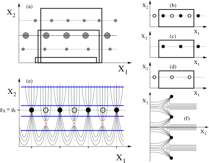
Figure 2: (a) Three representative pumping cycles. Several sets of Dirac monopoles may have non-zero weight depending on the occupation. Panel (b) is for single level occupation where two sets have non zero weight, while either (c) or (d) are for zero temperature Fermi occupation. Filled (hollow) circles indicate in(off)-plane monopoles. Panels (e-f) give a detailed illustration of the associated $\mathbf{B}$ field, as implied by the numerical findings of Figs.3-4. The $X_{1}$ tick marks in (e) are half De-Broglie spaced, while the horizontal blue lines are paths for which numerical results are presented in Figs. 3-4.

where $k_{\mbox{\tiny F}}=(2\mathsf{m}E_{\mbox{\tiny F}})^{1/2}$ is the Fermi momentum, and $\Delta X_{1}$ is the translation distance of the scatterer. Ref.avron has referred to this transport mechanism as “snow plow” and pointed out that it should be regarded as the prototype example for quantum pumping: a full pumping cycle (Fig. 2a) would consist of translating the scatterer to the right, shrinking its “size”, pulling it back to the left, and restoring its original size.

Quantum stirring pml ; pmt is the operation of inducing a DC circulating current by means of AC periodic driving. This is naturally achieved by integrating a quantum pump in a closed circuit pms ; pMB ; JJ . In particular Refs.pml ; pmt have considered the same adiabatic “snow plow” mechanism as described above and obtained for the model system of Fig. 1b the following result:

$$Q=\left[\frac{(1-g_{\mbox{\tiny X}})g_{\mbox{\tiny V}}}{g_{\mbox{\tiny X}}+g_{\mbox{\tiny V}}-2g_{\mbox{\tiny X}}g_{\mbox{\tiny V}}}\right]\frac{e}{\pi}k_{\mbox{\tiny F}}\ \Delta X_{1}$$ (2)

where $g_{\mbox{\tiny V}}$ is the transmission of the ring segment that does not include the moving scatterer, as defined by its Landauer conductance if it were connected to reservoirs.

Eq.(2) is “classical” in the Boltzmann sense because in its derivation the interference within the ring is ignored. The purpose of the present study is to derive quantum results for the stirring in a low dimensional device, where quantum mechanics has the most dramatic consequences. In particular we would like to illuminate the possibility of having a counter-stirring effect: by “pushing” the particles (say) anticlockwise, one can induce a circulating current in the counter-intuitive (clockwise) direction.

II Outline

As a preliminary stage we provide a simple pedagogical explanation of the counter-stirring effect by regarding the “pushing stage” of the pumping cycle as an adiabatic passage in multiple path geometry cnb .

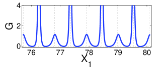
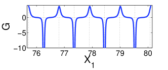
Figure 4: Additional plots of the conductance $G$ as calculated in the previous figure. The upper (lower) panel is for translation of a scatterer with ${g_{\mbox{\tiny X}}{=}0.20}$ (${g_{\mbox{\tiny X}}{=}0.03}$) corresponding to the horizontal blue paths in Fig. 2e that go below (above) the ${g_{\mbox{\tiny X}}{=}g_{\mbox{\tiny V}}}$ axis. Note that the large peaks are positive (negative) while the small positive peaks switch sign only when the scatterer is lowered further. This indicates that the field lines bend in the $X_{3}$ direction as illustrated in Fig.2f.

For the actual analysis in the general case we use the Kubo-Dirac monopoles picture of pmc . Within this framework the pumped charge $Q$ is determined by the flux of a $\bm{B}(X)$ field which is identified as the Berry-Kubo curvature berry1 ; avron2 ; berry2 . We study both analytically and numerically how this field looks like. The results are illustrated in Figs. 2-4. Summing the contributions of all the occupied levels we get expressions for the geometric conductance $G$. Integrating over a full pumping cycle we get results for $Q$.

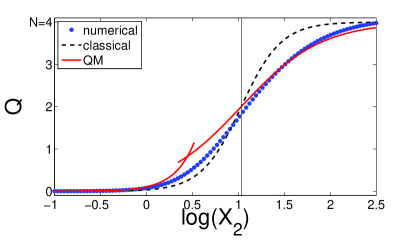
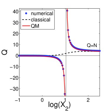
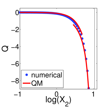
Figure 5: Numerical calculation of $Q$ for zero temperature Fermi occupation: all the levels are occupied up to $n{=}137$ (upper panel), and up to $n{=}138$ (lower regular and zoomed panels). The model parameters are the same as in Fig. 3. The integration was carried out along segments similar to the paths shown in Fig. 2e where $g_{\mbox{\tiny X}}$ varies between $g_{\mbox{\tiny X}}{=}8.30\cdot 10^{-5}$ and $g_{\mbox{\tiny X}}{=}0.45$. For sake of comparison we display both the analytical classical (Eq.2) and quantum results (Eqs.22&27). The value of $X_{2}$ for which $g_{\mbox{\tiny X}}{=}g_{\mbox{\tiny V}}$ is indicated by a vertical line.

We derive practical estimates for the stirring which is induced due to the translation of either small ($g_{\mbox{\tiny X}}\sim 1$) or a large ($g_{\mbox{\tiny X}}\ll 1$) scatterer, including the possibility of having $g_{\mbox{\tiny X}}\sim g_{\mbox{\tiny V}}$. The dependence of $Q$ on the size of the scatterer is plotted in Fig. 5, where it is contrasted with the classical expectation, and compared with the analytical approximations. In the Summary we refer to the experimental measurement aspect.

III The counter-stirring effect

The essence of the counter-stirring effect can be understood without the Kubo-Dirac monopoles picture by adopting the “splitting ratio” concept of Ref.cnb . Referring to Fig. 1b the translation of the scatterer to the right is effectively like lowering the potential floor in the left bond, and raising the potential floor in the right bond. This induces an adiabatic passage of a particle from the right to the left. The particle has two possible ways to make the passage: either via the “V” barrier (coupling $W_{12}^{\mbox{\tiny V}}$) or via the “X” barrier (coupling $W_{12}^{\mbox{\tiny X}}$). The splitting ratio determines the fraction of the current that goes via the “V” barrier:

$$\lambda(X_{2})=\frac{W_{12}^{V}}{W_{12}^{V}+W_{12}^{X}}={\frac{\sqrt{g_{\mbox{\tiny V}}}}{\sqrt{g_{\mbox{\tiny V}}}\pm\sqrt{g_{\mbox{\tiny X}}}}}$$ (3)

where the last equality is based on the analysis in Ref.pms . If $W_{12}$ were the classical rate of the transition, we would have ${0<\lambda<1}$ and the current would flow in accordance with our classical intuition. But $W_{12}^{\mbox{\tiny V}}$ and $W_{12}^{\mbox{\tiny X}}$ are real amplitudes that might have opposite signs if an odd level crosses an even level. Consequently if $|W_{12}^{\mbox{\tiny X}}|>|W_{12}^{\mbox{\tiny V}}|$ we get ${\lambda<0}$ which implies that a circulating current is induced in the counter-intuitive (clockwise) direction. This does not come in any contradiction with the observation that the net transport (summing over both barriers) is still from right to left.

IV The model Hamiltonian

Our model is a 1D coherent ring with a fixed scatterer and a controlled scatterer. The fixed scatterer is some potential barrier $V(x)$, and the controlled scatterer is modeled as a delta function whose position and transmission are determined by the control parameters $X_{1}$ and $X_{2}$ respectively. The one particle Hamiltonian is:

$${\cal H}=\frac{1}{2\mathsf{m}}\hat{p}^{2}+V(\hat{x})+X_{2}(t)\delta(\hat{x}-X_{1}(t))$$ (4)

with periodic boundary conditions over $x\in[-L/2,L/2]$ so as to have a ring geometry. Below we further assume that both bonds are of similar length (${L{-}X_{1}\sim X_{1}\sim L/2}$). The current is measured through a section $x{=}x_{0}{=}+0$ at the fixed barrier, and accordingly:

$${\cal I}=\frac{e}{2\mathsf{m}}\left(\hat{p}\delta(\hat{x}-x_{0})+\delta(\hat{x}-x_{0})\hat{p}\right)$$ (5)

We also define generalized forces which are associated with the control parameters:

$${\cal F}^{1}= -(\partial{\cal H}/\partial X_{1}) =X_{2}\delta^{\prime}(\hat{x}-X_{1})$$ (6)

$${\cal F}^{2}= -(\partial{\cal H}/\partial X_{2}) =-\delta(\hat{x}-X_{1})$$ (7)

For practical use it is more convenient to describe the fixed scatterer by its scattering matrix, which can be written as:

$${\bm{S}_{\mbox{\tiny V}}} = \mbox{e}^{i\gamma_{\mbox{\tiny V}}}\left(\begin{array}[]{cc}-i\sqrt{1-g_{\mbox{\tiny V}}}\mbox{e}^{i\alpha_{\mbox{\tiny V}}}&\sqrt{g_{\mbox{\tiny V}}}\\ \sqrt{g_{\mbox{\tiny V}}}&-i\sqrt{1-g_{\mbox{\tiny V}}}\mbox{e}^{-i\alpha_{\mbox{\tiny V}}}\end{array}\right)$$ (10)

We study the case when the model parameters are such that the transmission of the fixed scatterer is small ${(g_{\mbox{\tiny V}}\ll 1)}$, the Fermi momentum is large (${k_{\mbox{\tiny F}}L\gg 1}$), and the controlled scatterer is translated a distance $\Delta X_{1}$ that equals several Fermi wavelengths.

V The Kubo-Dirac picture

If we were changing the flux $X_{3}\equiv\Phi$ through the ring, the induced current would be given by Ohm law ${I=\langle\mathcal{I}\rangle=-G^{33}\dot{X_{3}}}$, where $G^{33}$ is the Ohmic conductance and $-\dot{X_{3}}$ is the electro-motive-force. Similarly for a variation of the parameter $X_{1}$, the current is $I=-G^{31}\dot{X}_{1}$, where $G^{31}$ is called the geometric conductance. For two parameters driving one can write:

$$Q=\int I\mbox{d}t=-\oint_{\mbox{cycle}}\bm{G}\cdot\mbox{d}\bm{X}=\oint\bm{B}\cdot\mbox{d}\bm{s}$$ (11)

where $\bm{G}=(G^{31},G^{32})$, and $\bm{X}=(X_{1},X_{2})$ and $\mbox{d}\bm{s}=(\mbox{d}X_{2},-\mbox{d}X_{1})$. For a particle that evolves adiabatically in the level $n$ we have ${G^{31}=B_{2}}$ and ${G^{32}=-B_{1}}$ where:

$$B_{j}^{(n)}=\sum_{m(\neq n)}\frac{2\ \mbox{Im}[{\cal I}_{nm}]{\cal F}^{j}_{mn}}{(E_{m}-E_{n})^{2}}$$ (12)

In fact $(B_{1},B_{2})$ are elements of the Kubo-Berry curvature berry1 ; avron2 ; berry2 which one can regard as a fictitious magnetic field $\vec{B}=(B_{1},B_{2},B_{3})$ in an embedding space ${X}=(X_{1},X_{2},X_{3})$. From the requirement of having well defined Berry phase it follows that the sources of $\vec{B}(X)$, which are located at points of degeneracy, are quantized, so called “Dirac monopoles”.

VI The $X$ space

Due to the gauge symmetry ${\Phi\mapsto\Phi+2\pi\hbar/e}$ the Dirac monopoles are arranged as vertical chains (see Fig. 2(f)) [${\hbar{=}e{=}1}$]. Due to the time reversal invariance of our $\mathcal{H}(X_{1},X_{2})$ it follows that a Dirac chain is either a duplication of in-plane monopole at ${X_{3}=0}$ or off-plane monopole at ${X_{3}=\pi}$. Let us find an explicit formula for the $(X_{1},X_{2})$ locations of these vertical chains. The equation for the adiabatic energies $E_{n}(X)$ is of the form $\cos(kL+\gamma)=\sqrt{g}\cos(\Phi)$ where $g$ is the total transmission of the ring and $\gamma$ is the total phase shifts of the scatterers (the fixed scatterers plus the moving scatterer). If $X_{2}$ is such that $g_{\mbox{\tiny X}}(E;X_{2})=g_{\mbox{\tiny V}}(E)$ we can always find $X_{1}$ such that the total transmission would be ${g=1}$, which is the necessary condition for having a degeneracy. Together with the equation ${k_{\mbox{\tiny E}}L+\gamma(E)=r\pi}$ with $r{=}\mbox{\small integer}$ this defines a set of energies ${E^{r}=(k^{r})^{2}/2\mathsf{m}}$ and associated values $X_{2}^{r}$ for which the $n{=}r$ level has degeneracy with the $n{=}r{+}1$ level provided $X_{1}$ is adjusted. To be more precise ${r{=}\mbox{\small even}}$ are in-plane ($\Phi{=}0$) degeneracies, while ${r{=}\mbox{\small odd}}$ are off-plane ($\Phi{=}\pi$) degeneracies. The $X_{1}$ locations of these degeneracies are half De-Broglie wavelength apart (see Fig.3):

$$X_{1}^{r}=\frac{\alpha_{\mbox{\tiny V}}}{2k^{r}}+\frac{L}{2}+\left(\left[\frac{1}{2}\right]+\mbox{\small integer}\right)\ \frac{\pi}{k^{r}}$$ (13)

where the $[1/2]$ shift applies to in-plane degeneracies. The arrangement of the degeneracies in $X$ space is illustrated in Fig.2. For each $(X_{1}^{r},X_{2}^{r})$ we have a vertical Dirac chain whose monopoles are formally like sources for the $\bm{B}$ field.

VII Fermi occupation

If we have many body system of $N=\sum_{n}f_{n}$ particles, then $\bm{B}=\sum_{n}f_{n}\bm{B}^{(n)}$. At finite temperature each occupied level (except $n{=}1$) contributes two sets of $(X_{1}^{r},X_{2}^{r})$ chains, namely $r{=}n$ and $r{=}n{-}1$, which are associated with the $E_{n}=E_{n{\pm}1}$ degeneracies. By inspection of Eq.(12), taking into account that $\mathcal{I}_{nm}$ is antisymmetric, one observes that the net contribution of the $r$th set of Dirac chains is ${f_{r}-f_{r{+}1}}$. In particular for zero temperature Fermi occupation, the net contributions comes from only one set of chains which is associated with the degeneracies of the last occupied level with the first non-occupied level (Fig. 2bcd).

VIII Classical limit

At finite temperatures we can define the smeared probability distribution of the Dirac monopoles with respect to $X_{2}$ as follows:

$$f(X_{2})\ =\ \overline{\sum_{r}[f_{r}-f_{r{+}1}]\,\delta(X_{2}-X_{2}^{r})}$$ (14)

Disregarding fluctuations Eq.(11) implies a monotonic dependence of $Q$ on $X_{2}$ in qualitative agreement with Eq.(2). If the expression in the square brackets of Eq.(2) were equal ${\int_{0}^{X_{2}}f(X^{\prime})dX^{\prime}}$, it would imply a quantitative agreement as well. In order to have this quantitative agreement we have to further assume that the distribution $f(X_{2})$ is determined by some chaotic dynamics in the scattering region which would imply erratic dependence of the $S$ matrix on the energy $E$. See pml for further discussion.

IX Quantum limit

Our interest below is in the opposite limit of zero temperature where $f(X_{2})$ becomes a step function. Obviously in this limit a step like behavior of $Q$ versus $X_{2}$ would be a crude approximation. By inspection of Eq.(12) it follows that the result for ${G\equiv G^{31}=B_{2}}$ is very well approximated by

$$G(X_{1},X_{2})=\frac{2\ \mbox{Im}[{\cal I}_{n,n{+}1}]{\cal F}^{1}_{n{+}1,n}}{(E_{n{+}1}-E_{n})^{2}}$$ (15)

where $n$ is the last occupied level. This observation, as well as the associated analytical results which are based on it, have been verified against the exact numerical results of Figs. 3-4. Below we derive explicit expressions for $G$ vs $X_{1}$ for both small and large values of $X_{2}$. Our results for $Q$ are plotted in Fig. 5. Note that the dependence on $X_{1}$ has $\pi/k_{\mbox{\tiny F}}$ periodicity due to the $X$ space arrangement of the monopoles, and accordingly the integration gives $Q\propto ek_{\mbox{\tiny F}}\Delta X_{1}/\pi$, with a prefactor that we would like to estimate.

X Matrix elements

The matrix elements of the current operator ${\cal I}$ and of the generalized force ${\cal F}^{1}$ are

$${\cal I}_{nm} = i\frac{e}{2\mathsf{m}}\left(\partial\psi^{(n)}\ \psi^{(m)}-\psi^{(n)}\ \partial\psi^{(m)}\right)$$ (16)

$${\cal F}^{1}_{mn} = -X_{2}\left(\overline{\partial\psi^{(m)}}\ \psi^{(n)}+\overline{\partial\psi^{(n)}}\ \psi^{(m)}\right)$$ (17)

$$= -\frac{1}{2\mathsf{m}}\left[\partial\psi_{R}^{(m)}\partial\psi_{R}^{(n)}-\partial\psi_{L}^{(m)}\partial\psi_{L}^{(n)}\right]$$

where $\overline{\partial\psi}=1/2(\partial\psi_{L}+\partial\psi_{R})$ is the average derivative on the left and right sides of the delta barrier, and the second expression for ${\cal F}^{1}_{nm}$ was obtained by using the matching conditions across the delta barrier. The wave function is written as ${\psi(x)=C\sin(\varphi+kx)}$. We found that a very good approximation for ${\cal I}_{nm}$ with $m{=}n{+}1$ is

$${\cal I}_{nm} = \pm ie\frac{v_{\mbox{\tiny F}}}{L}\sqrt{g_{\mbox{\tiny V}}}$$ (18)

where the $+$ $(-)$ sign is for $n=$even (odd), and $v_{\mbox{\tiny F}}=k_{\mbox{\tiny F}}/\mathsf{m}$ is the velocity in the energy range of interest. For the calculation of ${\cal F}^{1}_{mn}$ and $E_{m}-E_{n}$ we have to distinguish between the two cases of small/large scatter. This means the small/large $X_{2}$ regimes where $g_{\mbox{\tiny X}}\sim 1$ or $\ll 1$.

XI Translating a small scatterer

If the controlled scatterer is small, we treat it as a perturbation. For the energy splitting we get

$$E_{m}{-}E_{n}\approx\frac{\pi}{L}v_{\mbox{\tiny F}}\mp\frac{2}{L}X_{2}\cos(2k_{\mbox{\tiny F}}X_{1})$$ (19)

where for notational convenience we take $X_{1}^{r}$ as the new origin. After some further algebra we get

$${\cal F}^{1}_{mn}=\pm X_{2}\frac{2k_{\mbox{\tiny F}}}{L}\cos\left(2k_{\mbox{\tiny F}}X_{1}\right){+}X_{2}\frac{\pi}{L^{2}}$$ (20)

where the $\pm$ sign is as in Eq.(18). The conductance can be written as

$$G=\frac{e}{\pi}k_{\mbox{\tiny F}}\sum_{\nu=0}^{\infty}{\cal G}_{\nu}\cos\left(\nu\ 2k_{\mbox{\tiny F}}X_{1}\right)$$ (21)

where the coefficients of the leading non-negligible terms [the small parameter being $(1{-}g_{\mbox{\tiny X}})/g_{\mbox{\tiny X}}$] are

$${\cal G}_{0} = {\pm}2\sqrt{g_{\mbox{\tiny V}}}\left(\frac{1}{k_{\mbox{\tiny F}}L}\sqrt{\frac{1-g_{\mbox{\tiny X}}}{g_{\mbox{\tiny X}}}}{+}\frac{4}{\pi^{2}}\ {\frac{1-g_{\mbox{\tiny X}}}{g_{\mbox{\tiny X}}}}\right)$$ (22)

$${\cal G}_{1} = \frac{2}{\pi}\sqrt{g_{\mbox{\tiny V}}}\ \left(\frac{4}{k_{\mbox{\tiny F}}L}{\frac{1-g_{\mbox{\tiny X}}}{g_{\mbox{\tiny X}}}}{+}2\sqrt{\frac{1-g_{\mbox{\tiny X}}}{g_{\mbox{\tiny X}}}}\right)$$ (23)

Upon integration we get $Q=-e\,{\cal G}_{0}$ per half Fermi wavelength displacement of the scatterer.

XII Translating a large scatterer

If the controlled scatterer is large, most of the charge transfer is induced during the avoided crossings (sharp peaks in Fig. 3 lower panel). Consequently we use the two level approximation scheme of pms with $m=n{+}1$ leading to the results:

$$E_{m}-E_{n} = \frac{2}{L}v_{\mbox{\tiny F}}\ |{\bm{R}}|$$ (24)

$${\cal F}^{1}_{mn} = \pm\frac{2}{L}\mathsf{m}{v_{\mbox{\tiny F}}^{2}}\ \frac{R_{2}}{|{\bm{R}}|}$$ (25)

where the $\pm$ sign is as in Eq.(18) and the dimensionless distance in ${\bm{X}}$ space from the degeneracy point is:

$${\bm{R}} = \left(2k_{\mbox{\tiny F}}(X_{1}-X_{1}^{r}),\ \frac{\sqrt{g_{\mbox{\tiny V}}}}{\lambda(X_{2})}\right)$$ (26)

Accordingly the conductance is

$$G=e\frac{k_{\mbox{\tiny F}}}{\sqrt{g_{\mbox{\tiny V}}}}\ \frac{R_{2}}{|{\bm{R}}|^{3}}$$ (27)

Integrating over $X_{1}$ we get $Q=e\lambda(X_{2})$ per half Fermi wavelength displacement of the scatterer, as expected from the “splitting ratio” argument.

XIII Summary

The integration of a two-terminal quantum pump in a closed circuit is not a straightforward procedure. Due to interference the pumped charge $Q$ would not be the same as in the Landauer/BPT setup, and even the sense of the induced current might be reversed. The most dramatic consequences would be observed in low dimensional devices. For this reason we have analyzed in this paper the prototype problem of “pushing” a current by translating a scatterer in a single mode wire. We have obtained explicit results for the $\bm{B}$ field, which determines the geometric conductance $G$, and consequently the $Q$ of a closed pumping cycle. We also illuminated the counter-stirring effect using the splitting ratio concept of adiabatic passage in multiple path geometry.

A few words are in order regarding the measurement procedure and the experimental relevance. It should be clear that to measure current in a closed circuit requires special techniques orsay ; expr1 ; expr2 . These techniques are typically used in order to measure persistent currents, which are zero order (conservative) effect, while in the present paper we were discussing driven currents, which are a first-order (geometric) effect. It is of course also possible to measure the dissipative conductance (as in orsay ). During the measurement the coupling to the system should be small. These are so called weak measurement conditions. More ambitious would be to measure the counting statistics, i.e. also the second moment of $Q$ as discussed in cnb ; cnz which is completely analogous to the discussion of noise measurements in open systems levitov ; nazarov . Finally it should be pointed out that the formalism above, and hence the results, might apply to experiments with superconducting circuits (see JJ ).

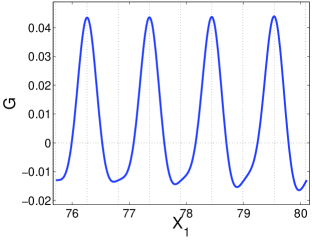
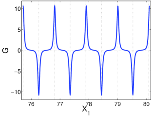
Figure 3: The conductance $G{=}G^{31}$ of Eq.12 is numerically calculated for a ring of length $L{=}151.43$ with $V(x){=}U\delta(x)$ where $U{\sim}10$. We consider single level occupation $n{=}138$. At this energy ${g_{\mbox{\tiny V}}{=}0.06}$. The upper (lower) panel is for translation of a very small (large) scatterer with ${g_{\mbox{\tiny X}}{=}0.98}$ (${g_{\mbox{\tiny X}}{=}8\cdot 10^{-8}}$) corresponding to the lower (upper) horizontal blue paths that are indicated in Fig. 2e (same $X_{1}$ axis).

- (1) J. E. Avron, A. Elgart, G. M. Graf and L. Sadun, Phys. Rev. B 62 (2000) 10618
- (2) M. Buttiker, H. Thomas and A. Pretre, Z. Phys. B 94 (1994) 133
- (3) P. W. Brouwer, Phys. Rev. B 58 (1998) 10135
- (4) G. Rosenberg and D. Cohen, J. Phys. A 39 (2006) 2287
- (5) D. Cohen, T. Kottos and H. Schanz, Phys. Rev. E 71 (2005) 035202(R)
- (6) I. Sela and D. Cohen, J. Phys. A 39 (2006) 3575
- (7) M. Moskalets and M. Büttiker, Phys. Rev. B 68 (2003) 161311
- (8) M. Mottonen, J. P. Pekola, J. J. Vartiainen, V. Brosco and F. W. J. Hekking, Phys. Rev. B 73 (2006) 214523
- (9) M. Chuchem and D. Cohen, J. Phys. A 41, 075302 (2008).
- (10) D. Cohen, Phys. Rev. B 68 (2003) 155303
- (11) M.V. Berry, Proc. R. Soc. Lond. A 392 (1984) 45
- (12) J. E. Avron, A. Raveh and B. Zur, Rev. Mod. Phys. 60 (1988) 873
- (13) M.V. Berry and J.M. Robbins, Proc. R. Soc. Lond. A 442 (1993) 659
- (14) Measurements of currents in arrays of closed rings are described by: B. Reulet M. Ramin, H. Bouchiat and D. Mailly, Phys. Rev. Lett. 75, 124 (1995).
- (15) Measurements of currents in individual closed rings using SQUID is described in: N.C. Koshnick, H. Bluhm, M.E. Huber, K.A. Moler, Science 318, 1440 (2007).
- (16) A new micromechanical cantilevers technique for measuring currents in closed rings is described in: A.C. Bleszynski-Jayich, W.E. Shanks, R. Ilic, J.G.E. Harris, arXiv:0710.5259.
- (17) M. Chuchem and D. Cohen, Phys. Rev. A 77, 012109 (2008).
- (18) L.S. Levitov and G.B. Lesovik, JETP Letters 58, 230 (1993).
- (19) Y.V. Nazarov and M. Kindermann, European Physical Journal B 35, 413 (2003).