3D Computer Simulations of Pulsatile Human Blood Flows in Vessels and in the Aortic Arch: Investigation of Non-Newtonian Characteristics of Human Blood

Abstract

Methods of Computational Fluid Dynamics are applied to simulate pulsatile blood flow in human vessels and in the aortic arch. The non-Newtonian behaviour of the human blood is investigated in simple vessels of actual size. A detailed time-dependent mathematical convergence test has been carried out. The realistic pulsatile flow is used in all simulations. Results of computer simulations of the blood flow in vessels of two different geometries are presented. For pressure, strain rate and velocity component distributions we found significant disagreements between our results obtained with realistic non-Newtonian treatment of human blood and widely used method in literature: a simple Newtonian approximation. A significant increase of the strain rate and, as a result, wall sear stress distribution, is found in the region of the aortic arch. We consider this result as theoretical evidence that supports existing clinical observations and those models not using non-Newtonian treatment underestimate the risk of disruption to the human vascular system.

Keywords: Fluid dynamics, Navier-Stokes equation, human blood flow, non-Newtonian viscosity, human vessels, aortic arch, pressure and wall shear stress distributions.

1 . Introduction

Human blood is a liquid with variable density and viscosity. The movement of the blood inside vessels and arteries can be described by fundamental laws of physics, i.e. equations of fluid dynamics. The scientific literature now contains many citations where researchers have used computer simulations of blood flows in various size vessels and arteries at different spatial geometries, see for example [1-10]. Whereas experimental investigations of vascular dynamics and flow are complicated or simply impossible to carry out due to small sizes of vessels in living systems. Therefore, theoretical-mathematical models and computer simulations are very useful for studying blood flows.

Atherosclerosis occurs at specific arterial sites. This phenomenon is related to hemodynamics and to wall shear stress (WSS) distributions. WSS is the tangential drag force produced by moving blood. It is a mathematical function of the velocity gradient of blood near the endothelial surface: $\tau_{w}=\mu\left[\partial U(t,y,R_{v})/\partial y\right]_{y\approx 0,}$ here $\mu$ is the dynamic viscosity, $t$ is current time, $U(t,y,R_{v})$ is the flow velocity parallel to the wall, $y$ is the distance to the wall of the vessel, and $R_{v}$ is its radius. It was shown, that the magnitude of WSS is directly proportional to blood flow and blood viscosity and inversely proportional to the cube of the radius of vessels, in other words a small change of the radius of a vessel will have a large effect on WSS.

Arterial wall remodeling is regulated by WSS. In response to high shear stress arteries enlarge. Consequently, the atherosclerotic plaques localize preferentially in regions of low shear stresses, but not in regions of higher shear stresses. Furthermore, decreased shear stress induces intimal thickening in vessels which have adapted to high flow. Also, final vascular events that induce fatal outcomes, such as acute coronary syndrome, are triggered by the sudden mechanical disruption of an arterial wall. Thus, we can conclude, that the final consequences of tragic fatal vascular diseases are strongly connected to mechanical events that occur on the vascular wall, and these, in turn, which are likely to be heavily influenced by alterations in blood flow and the characteristics of the blood itself.

In order to predict, diagnose, and prevent fatal outcomes in these vascular diseases, fluid + solid mechanical interactions between the human blood and the vascular wall are attractive and necessary targets for analysis. However, it is very difficult to make measurements of detailed mechanical properties in living systems. In turn, theoretical bio-mathematics provides a series of logic tools that can overcome limitations of direct measurements in highly labile living systems and provide a framework for testing variables, and is more rapid, efficient, and possibly more predictive than repeated experimentation in animal modeling systems

In this work we carry out real-time full-dimensional computer simulations of pulsatile blood flows in actual size vessels and in the aortic arch. We take into account different physical effects on blood flow and examine the non-Newtonian nature of human blood as a fluid.

Computer simulation is well-suited to those cases in which it is difficult to carry out reliable experiments due to the very small size of some vessels, such as, for example, coronary arteries. Also, bio-mathematical computer simulations may be especially useful in situations when an intravascular stent is implanted inside a vessel, aortic arch, aortas etcetera. Stents may have complicated shapes and they are very small micro-devices (typically only several millimeters in diameter, when fully deployed). It is useful to know pressure, strain rate distributions and the profile of blood flow after coming through a stented vessel.

The next section presents the mathematical and numerical methods used in this work. Section 3 presents our results. The CGS unit system is used in all simulations as well as for presentation of our results.

2 . Method

In this work we consider the human blood as an incompressible fluid, and flows in vessels and in the aortic arch are assumed to be laminar. One of the goals of this work is to investigate the non-Newtonian behaviour of the human blood. To attain these ends we carry out simulations for same systems, but with different models of the blood. Then we compare the results.

For many years, investigation of hemorheology has been of great interest in the field of biomedical engineering. Researchers have investigated correlations for example, of stroke, arterial diseases, hypertension, and whole blood viscosity. Blood consists of plasma and particles, including red blood cells, leukocytes, platelets and macromolecular protein aggregates. The viscosity of blood depends on the viscosity of plasma, in combination with the hematocrit (a measure of the particulate component of blood). The normal hematocrit of human blood ranges between 35% - 45%. Higher hematocrit implies higher viscosity. The relation between hematocrit and viscosity is very complex and in the scientific literature, many mathematical fitting formulas are available for assessing this relationship.

Next, the viscosity of blood determines its velocity. That is, when velocity or shear rate increases viscosity decreases. Also, the viscosity/velocity depends on the size of the blood vessel. This is called the Fahraeus-Lindqvist effect, that is in small diameter blood vessels, and at higher velocities, blood viscosity decreases. Viscosity of human blood strongly depends on its temperature.

To carry out our simulations we used a commercial program FLOW3D from Flow Science Inc., Santa Fe, New Mexico, USA. FLOW3D is a general purpose CFD package. It applies specially developed numerical techniques to solve the equations of motion of fluid. The methods implemented in the program allow us to obtain transient, 3D solutions for multi-scale and multi-physics flow problems. One of the most attarctive sides of FLOW3D is very well developed numerical techniques to solve non-linear fluid dynamic equations. To our best knowledge our work is the first time application of the FLOW3D program to blood flows in human vessels.

When the turbulence option is used, the viscosity is a sum of the molecular and turbulent values. For non-Newtonian fluids the viscosity can be a function of the strain rate and/or temperature. A general expression based on the Carreau model is used in FLOW-3D for the strain rate dependent viscosity:

$$\mu=\mu_{\infty}+\frac{\mu_{0}E_{T}-\mu_{\infty}}{\lambda_{00}+[\lambda_{0}+(\lambda_{1}E_{T})^{2}e_{ij}e_{ij}]^{(1-n)/2}}$$

$$+\frac{\lambda_{2}}{\surd(e_{ij}e_{ij})},$$ (1)

where $e_{ij}=1/2(\partial u_{i}/\partial x_{j}+\partial u_{j}/\partial x_{i})$ is the fluid strain rate in Cartesian tensor notations, $\mu_{\infty},\mu_{0},\lambda_{0},\lambda_{1},\lambda_{2}$ and $n$ are constants. Also, $E_{T}=exp[a(T^{*}/(T-b)-C)],$ where $T^{*},a,b,$ and $c$ are also parameters of the temperature dependence, and $T$ is fluid temperature. This basic formula is used in our simulations for blood flow in vessels and in the aortic arch.

Next, fluid dynamics is described with 2-nd order non-linear, transient differential equations. The governing equations consist of the continuity equation and the Navier-Stokes equations. The general mass continuity equation, which is solved within the FLOW3D program has the following general form:

$$V_{f}\frac{\partial\rho}{\partial t}+\frac{\partial}{\partial x}(\rho uA_{x})+R\frac{\partial}{\partial y}(\rho vA_{y})+\frac{\partial}{\partial z}(\rho wA_{z})+$$

$$\xi\frac{\rho uA_{x}}{x}=R_{dif}+R_{sor},$$ (2)

where $V_{F}$ is the fractional volume open to flow, $R$ and $xi$ are coefficients which value dependent on the coordinate system: $(x,y,z)$ or $(r,\theta,z)$, $\rho$ is the fluid density, $R_{dif}$ is a turbulent diffusion term, and $R_{sor}$ is a mass source, $(u,v,w)$ are the velocity components in coordinate directions $(x,y,z)$ respectively. For example, when Cartesian coordinates are used, $R=1$ and $\xi=0$, see FLOW3D manual [9]. Finally, $A_{x}$ is the fractional area open to flow in the $x$ direction, analogously for $A_{y}$ and $A_{z}$.

The turbulent diffusion term is

$$R_{dif}=\frac{\partial}{\partial x}(v_{p}A_{x}\frac{\partial\rho}{\partial x})+R\frac{\partial}{\partial y}(v_{p}A_{y}R\frac{\partial\rho}{\partial y})+$$

$$\frac{\partial}{\partial z}(v_{p}A_{z}\frac{\partial\rho}{\partial z})+\xi\frac{\rho v_{p}A_{x}}{x},$$ (3)

where the coefficient $v_{p}=C_{p}\mu/\rho$, $\mu$ is dynamic viscosity and $C_{p}$ is a constant. The $R_{sor}$ term is a density source term that can be used to model mass injections through porous obstacle surfaces.

It is well known, that compressible flow problems require solution of the full density transport equation. In this work we treat blood as an incompressible fluid. For incompressible fluids $\rho=constant$ and the Eqn. (2) becomes the following:

$$\frac{\partial}{\partial x}(uA_{x})+\frac{\partial}{\partial y}(vA_{y})+\frac{\partial}{\partial z}(wA_{z})+\xi\frac{uA_{x}}{x}=\frac{R_{sor}}{\rho}.$$ (4)

The equations of motion for the fluid velocity components $(u,v,w)$ in the 3-coordinate system are the Navier-Stokes equations with specific additional terms included in the FLOW3D program:

$$\frac{\partial u}{\partial t}+\frac{1}{V_{F}}{uA_{x}\frac{\partial u}{\partial x}}+{vA_{y}\frac{\partial u}{\partial x}}+{wA_{z}\frac{\partial u}{\partial x}}-\xi\frac{A_{y}v^{2}}{xV_{f}}=$$

$$-\frac{1}{\rho}\frac{\partial p}{\partial x}+G_{x}+f_{x}-b_{x}-\frac{R_{sor}}{\rho V_{f}}(u-u_{w}-\delta\cdot u_{s})$$ (5)

$$\frac{\partial u}{\partial t}+\frac{1}{V_{F}}{uA_{x}\frac{\partial u}{\partial x}}+{vA_{y}\frac{\partial u}{\partial x}}+{wA_{z}\frac{\partial u}{\partial x}}+\xi\frac{A_{y}uv}{xV_{f}}=$$

$$-\frac{1}{\rho}R\frac{\partial p}{\partial y}+G_{y}+f_{y}-b_{y}-\frac{R_{sor}}{\rho V_{f}}(v-v_{w}-\delta\cdot v_{s})$$ (6)

$$\frac{\partial u}{\partial t}+\frac{1}{V_{F}}{uA_{x}\frac{\partial u}{\partial x}}+{vA_{y}\frac{\partial u}{\partial x}}+{wA_{z}\frac{\partial u}{\partial x}}=-\frac{1}{\rho}\frac{\partial p}{\partial z}+$$

$$G_{z}+f_{z}-b_{z}-\frac{R_{sor}}{\rho V_{f}}(w-w_{w}-\delta\cdot w_{s}),$$ (7)

where, $(G_{x},G_{y},G_{z})$ are so called body accelerations [9], $(f_{x},f_{y},f_{z})$ are viscous accelerations, $(b_{x},b_{y},b_{z})$ are flow losses in porous media or across porous baffle plates, and the final term accounts for the injection of mass at a source represented by a geometry component. As we mentioned above, FLOW3D is a general purpose fluid dynamics program, which includes many specific situations. However, in this short description we try to make a valuable impression about FLOW3D and give here the general form of all equations. Next, the term $U_{w}=(u_{w},v_{w},w_{w})$ in Eqn. (5) is the velocity of the source component, which will generally be non-zero for a mass source at a General Moving Object (GMO) [9]. The term $U_{s}=(u_{s},v_{s},w_{s})$ is the velocity of the fluid at the surface of the source relative to the source itself. It is computed in each control volume as

$$\vec{U}_{s}=\frac{1}{\rho_{s}}\frac{d(Q\vec{n})}{dA}$$ (8)

where $dQ$ is the mass flow rate, $\rho_{s}$ fluid source density, $dA$ the area of the source surface in the cell and $\vec{n}$ the outward normal to the surface.

The source is of the stagnation pressure type when in Eqs. (5-7) $\delta=0.0$. Next, $\delta=1.0$ corresponds to the source of the static pressure type.

It is assumed, that at a stagnation pressure source fluid enters the domain at zero velocity. As a result, pressure should be considered at the source to move the fluid away from the source. For example, such sources are designed to model fluid emerging at the end of a rocket or the simple deflating process of a balloon. In general, stagnation pressure sources apply to cases when the momentum of the emerging fluid is created inside the source component, like in a rocket engine. At a static pressure source the fluid velocity is computed from the mass flow rate and the surface area of the source. In this case, no extra pressure is required to propel the fluid away from the source. An example of such a source is fluid emerging from a long straight pipe. Note that in this case the fluid momentum is created far from where the source is located.

For a variable dynamic viscosity $\mu$, the viscous accelerations are

$$\rho V_{F}f_{x}=w^{s}_{x}-(\frac{\partial}{\partial x}(A_{x}\tau_{xx})+R\frac{\partial}{\partial y}(A_{y}\tau_{xy})+$$

$$\frac{\partial}{\partial z}(A_{z}\tau_{xz})+\frac{\mu}{x}(A_{x}\tau_{xx}-A_{y}\tau_{yy}))$$ (9)

$$\rho V_{F}f_{y}=w^{s}_{y}-(\frac{\partial}{\partial x}(A_{x}\tau_{xy})+R\frac{\partial}{\partial y}(A_{y}\tau_{yy})+$$

$$\frac{\partial}{\partial z}(A_{z}\tau_{yz})+\frac{\mu}{x}(A_{x}+A_{y}\tau_{xy}))$$ (10)

$$\rho V_{F}f_{z}=w^{s}_{z}-\left(\frac{\partial}{\partial x}(A_{x}\tau_{xz})+R\frac{\partial}{\partial y}(A_{y}\tau_{yz})\right)+$$

$$\left(\frac{\partial}{\partial z}(A_{z}\tau_{zz})+\frac{\mu}{x}(A_{x}\tau_{xz})\right),$$ (11)

where

$$\tau_{xx}=-2\mu\left(\frac{\partial u}{\partial x}-\frac{1}{3}\left(\frac{\partial u}{\partial x}+R\frac{\partial v}{\partial y}+\frac{\partial w}{\partial z}+\frac{\xi u}{x}\right)\right)$$ (12)

$$\tau_{yy}=-2\mu\left(\frac{\partial v}{\partial x}+\xi\frac{u}{x}\right)$$

$$-\frac{1}{3}\left(\frac{\partial u}{\partial x}+R\frac{\partial v}{\partial y}+\frac{\partial w}{\partial z}+\frac{\xi u}{x}\right)$$ (13)

$$\tau_{zz}=-2\mu\left(\frac{\partial w}{\partial z}-\frac{1}{3}\left(\frac{\partial u}{\partial x}+R\frac{\partial v}{\partial y}+\frac{\partial w}{\partial z}+\frac{\xi u}{x}\right)\right)$$ (14)

$$\tau_{xy}=-\mu\left(\frac{\partial v}{\partial x}+R\frac{\partial u}{\partial y}-\frac{\xi v}{x}\right)$$ (15)

$$\tau_{xz}=-\mu\left(\frac{\partial u}{\partial z}+\frac{\partial w}{\partial x}\right)$$ (16)

$$\tau_{yz}=-\mu\left(\frac{\partial v}{\partial z}+R\frac{\partial w}{\partial y}\right).$$ (17)

In Eqs. (12)-(17) the terms $w^{s}_{x},w^{s}_{y}$ and $w^{s}_{z}$ are wall shear stresses. If these terms are equal to zero, there is no wall shear stress. This is because the remaining terms contain the fractional flow areas $(A_{x},A_{y},A_{z})$ which vanish at the walls. The wall stresses are modeled by assuming a zero tangential velocity on the portion of any area closed to flow. Mesh and moving obstacle boundaries are an exception because they can be assigned non-zero tangential velocities. In this case the allowed boundary motion corresponds to a rigid body translation of the boundary parallel to its surface. For turbulent flows, a law-of-the-wall velocity profile is assumed near the wall, which modifies the wall shear stress magnitude.

As we already mentioned, in all simulations we consider the blood flow as pulsatile flow. The final result for the inflow waveform has been taken from work [6]. The waveform is shown in Fig. 1. These velocity values are used as time-dependent inflow initial boundary conditions. These numbers are included directly in the FLOW3D program.

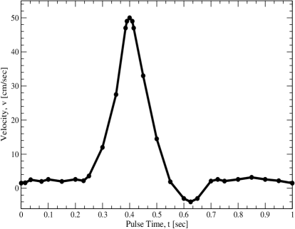
Figure 1: Velocity waveform at the vessel inlet. Results taken from Fig. 2 of work [6].

The equations of fluid dynamics should be solved together with specific boundary conditions. The numerical model starts with a computational mesh, or grid. It consists of a number of interconnected elements, or 3D-cells. These 3D-cells subdivide the physical space into small volumes with several nodes associated with each such volume. The nodes are used to store values of the unknown parameters, such as pressure, strain rate, temperature, velocity components etcetera. This procedure provides values for defining the flow parameters at discrete locations and to set up specific boundary conditions. Finally, one can start developing effective numerical approximations for the solution of the fluid dynamics equations.

New pressure-velocity solvers have been implemented in FLOW-3D. We used the so called GMERS method. GMRES stands for the generalized minimum residual method. In addition to the GMRES solver, a new optional algorithm, the generalized conjugate gradient (GCG) algorithm, has also been implemented for solving viscous terms in the new GMRES solver. This new solver is a highly accurate and efficient method for a wide range of problems. It possesses good convergence, symmetry and speed properties; however, it does use more memory than the SOR or SADI methods. The GMRES solver does not use any over- or under-relaxation [9].

3 . Results

This section represents the results of our simulations for blood flows in a simple vessel and in the human aortic arch. The first geometry was chosen for preliminary test calculations and testing the FLOW3D program. One of the most important preliminary testing tasks is the check numerical convergence. This test has been successful and our results will be shown below in this paper. To our best knowledge the current work is a first attempt to apply FLOW3D to human blood flows in vessels and in aortic arch.

First, we present results for a simpler geometry vessel in the shape of a tube. However, the human blood is treated as real and a non-Newtonian liquid. The necessary data for viscosity of the blood we found from previous laboratory and clinical measurements [1, 3]. We take into account the real pulsatile flow, which is shown in Fig. 1. The data for Fig. 1 have also been obtained in clinical measurements [6].

After such preliminary simulations we switch to a more complicated spatial configuration. In this work it is the aortic arch. It is axiomatic that real people may have different size aortic arches with slightly different shapes. However, we carried out simulations for an average size and shape aortic arch.

The main goal of this work is to treat the above mentioned systems realistically, reveal the physics of the blood flow dynamics, and to obtain reliable results for pressure, dynamic viscosity, velocity profiles and strain rate distributions. Also, we tested, the widely cited in literature, Newtonian and non-Newtonian models of the human blood.

3.1 Blood flow in vessel

As we mentioned above in this work we adopted the shape of a straight vessel as a tube. The sizes of the tube are: $L=8$ cm in length and $R=0.34$ cm in the inner radius. The thickness of the vessel wall is $s=0.03$ cm. We have chosen 5.5 cycles of the blood pulse.

Consider in more detail the expression (1). In these calculations we follow the works [1, 3], where the Carreau model of the human blood has also been used. In consistence with [1, 3] we choose the following coefficients: $\lambda_{2}=\lambda_{00}=0$, $a=0$ and $E_{T}=1$, that is we don’t take into account the temperature dependence of the viscosity. Next: $\lambda_{0}=1$, $\lambda_{1}=3.313$ sec, $\mu_{\infty}=0.0345$ P, $\mu_{0}=0.56$ P, and $n=0.3568$.

In our calculations we applied a cylindrical coordinate system with the axis $OZ$ directed over the tube axis. Different numbers of cells have been used to discretize the empty space inside the tube. In the open space (inner part of the tube) the fluid dynamics equations have been solved together with appropriate mathematical boundary conditions. The convergence was achieved when we used 52,800 cells, that is we used 100 points over $OZ$, 22 points over the radius of the inside space $R=0.34$ cm, and 24 points over azimuthal angle $\Phi$ from 0 to 2$\pi$.

Time-dependent results for pressure, strain rate and velocity component $W$ are presented in Fig. 2. We chose three precise geometrical points to compare results - 1st: in the inlet of the tube, when $Z=0$; 2nd: in the middle point $Z=4.0$ cm, and 3rd: in outlet point $z=8.0$ cm. The data for Fig. 2 was obtained with two different models of human blood. The bold lines are results with the non-Newtonian viscosity (1) and the dashed lines are results with the Newtonian model when the viscosity $\mu$ has a constant value and equals to 0.0345 P. As one can see the results are different for strain rate distributions and very different for pressure distributions. These results clearly indicate that probably in most cases of computer simulations of human blood flows only the non-Newtonian model should be used.

In Fig. 3 we show our time-dependent convergence results. These data are obtained with the realistic non-Newtonian model of the blood. Again, we have chosen three geometrical points to compare results: 1- in the inlet of the tube, when $Z=0$; 2- in the middle point $Z=4.0$ cm, and 3- outlet point $z=8.0$ cm.

Three upper rows represent time-dependent plots for pressure, dynamics viscosity and strain rate distributed over the simulation time, which is 5.5 sec. However, below in three lower rows results for the kinematic characteristics of the blood flow are also shown, which are three components of the blood velocity: $U,V,W$. The results are obtained with three sets of computation cell distributions, where we used 36,000 cubic cells, 47,000 and 52,000 cubic cells. As we see from Fig. 3 it is harder to obtain convergence for the pressure distributions and easier for other shown parameters.

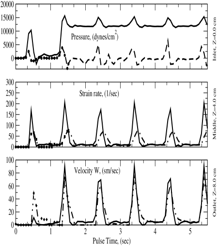
Figure 2: Time-dependent pressure, strain rate and velocity component W - over OZ axis. Results for straight vessel for 3 spatial points: Z=0, 4, 8 cm. Bold lines: calculations with realistic non-Newtonian viscosity of human blood. Dashed lines: simple Newtonian approximation.

3.2 Blood flow in aortic arch

The aortic arch is represented as a curved tube [4]. In our simulations the outer radius of the tube is 2.6 cm. A straight vessel (tube) is also merged to the arch. The length of the straight tube is about 4 cm. Again, the thickness of the wall is 0.03 cm, and the inner radius of the tube is $r=0.34$ cm. The geometry is shown in Figs. 4 and 5. This configuration closely models and represents the real aortic arch. One of the goals of these simulations is to reveal the physics of the blood flow dynamics in the arch.

Now we use the Cartesian coordinate system. Here we also carried out a convergence test. To better represent the shape of the arch we applied five Cartesian sub-coordinate systems in our FLOW3D simulations. After the discretization the total number of all cubic cells reached about 400,000. It is important to mention here, that we again obtained a full numerical convergence.

As we mentioned the goal of these simulations is to compute pressure, velocity and strain rate distributions in the arch, while the human blood is treated as a non-Newtonian liquid and the realistic pulsatile blood flow is used as it is shown in Fig. 1. In Figs. 4 and 5 we show the results for strain rate distributions inside the arch for four specific time moments. At the most left point, which is inlet, we specify the pulsatile velocity source as the initial condition, that is the data from Fig. 1 are used. From the general theory of fluid mechanics [10] it is possible to determine together with viscosity and spatial geometry, the dynamics of the blood according to the Navier-Stokes equation and its boundary conditions. Small vectors indicate the blood velocity. As can be seen blood flows from left to right in direction. However, because of pulsatility blood flows in the opposite direction too. It is seen in Fig. 4 - lower right graph # 43. It is in good agreement with the general physical intuition, and it additionally shows correctness of these simulations.

The values of the strain rate are also shown. These values are strongly oscillating. From the plots one can conclude that in the region of the arch the strain rate values are becoming much larger than in the region of the straight vessel. This result represents clear evidence that in this part of the human vascular system atherosclerotic plaques should localize less than in the straight vessels. However, the higher wall shear stress values in the aortic arch could be the reason for sudden mechanical disruption of the arterial wall in this part of the human vascular system. These results are consistent with laboratory and clinical observations.

In conclusion, we would like to point out here, that the developments in this work can be directly applied to even more interesting and important situation such as, when a stent is implanted inside a vessel [5, 7, 8]. In that case, for example, it is important to determine blood flow disturbance, the pressure distribution, strain rate and etcetera. This work is in progress in our group.

Figure 4. Blood flow in the aortic arch for two consecutive moments of the discretized time. A strong pulsatility of the strain rate values is seen: Upper plot shows results for t = 4.218 sec, where strain rate ranges from e = 1.1 1/sec to e = 24.6 1/sec. Lower plot shows results for t = 4.329 sec, where strain rate ranges from e = 5. 1/sec to e=234. 1/sec. The maximum values of the strain rate are localized in the region inside the arch. Blood flows from right to left in both pictures.

Figure 5. Blood flow in the aortic arch for two consecutive moments of discretized time. Upper plot shows results for t = 4.551 sec, where strain rate ranges from e = 0.4 1/sec to e = 22.6 1/sec. Lower plot shows results for t = 4.662 sec, where strain rate ranges from e = 0.1 1/sec to e = 27.6 1/sec. The maximum values of the strain rate are localized again in the region inside the arch. In the upper plot blood flows from left to right, however in the lower plot: from right to left.

References

- [1] Y.I. Cho, K.R. Kensey, Effects of the non-Newtonian viscosity of blood on flows in a diseased arterial vessel. Part 1: Steady Flows, Biorheology 28, 241-262 (1991).
- [2] Taylor, C.A., Draney, M.T., Experimental and Computational Methods in Cardiovascular Fluid Mechanics, Annual Review of Fluid Mechanics 36, 197-231 (2004).
- [3] Johnson, B.M., Johnson, P.R., Corney, S., and Kilpatrick, D., Non-Newtonian Blood Flow in Human Right Coronary Arteries: Steady State Simulations, J. of Biomech. 37, 709 (2004).
- [4] Morris, L., Delassus, P., Callan, A., Walsh, M., Wallis, F., Grace, P., McGloughlin, T., 3-D Numerical Simulation of Blood Flow Through Models of the Human Aorta, J. Biomechanical Engineering 127, 767-775 (2005).
- [5] Duraiswamy, N., Schoephoerster, R.T., Moreno, M.R., Moore Jr., J.E., Stented Artery Flow Patterns and Their Effects on the Artery Wall, Annual Review of Fluid Mechanics 39, 357-382 (2007).
- [6] Y. Papaharilaou, J.A. Ekaterinaris, E. Manousaki, A.N. Katsamouris, A Decoupled Fluid Structure Approach for Estimating Wall Stress in Abdominal Aortic Aneurysms, J. Biomechanics 40, 367-377 (2007).
- [7] Faik, I., Mongrain, R., Leask, R.L., Rodes-Cabau, J., Larose, E., Bertrand, O., Time-Dependent 3D Simulations of the Hemodynamics in a Stented Coronary Artery, Biomedical Materials 2 (1), art. no. S05, S28-S37 (2007).
- [8] Banerjee, R.K., Devarakonda, S.B., Rajamohan, D., Back, L.H., Developed Pulsatile Flow in a Deployed Coronary Stent, Biorheology 44 (2), 91-102 (2007).
- [9] FLOW-3D Users Manual, Version 9.2, Flow Science, Santa Fe, New Mexico, 2007.
- [10] Landau, L.D., Lifshitz, E.M., Fluid Mechanics, Volume 6, Pergamon Press Ltd., 1959.