Disorder induced transverse delocalisation in ropes of carbon nanotubes.

Abstract

A rope of carbon nanotubes is constituted of an array of parallel single wall nanotubes with nearly identical diameters. In most cases the individual nanotubes within a rope have different helicities and 1/3 of them are metallic. In the absence of disorder within the tubes, the intertube electronic transfer is negligeable because of the longitudinal wave vector mismatch between neighboring tubes of different helicities. The rope can then be considered as a number of parallel independent ballistic nanotubes. On the other hand, the presence of disorder within the tubes favors the intertube electronic transfer. This is first shown using a very simple model where disorder is treated perturbatively inspired by the work in reference maarouf00 . We then present numerical simulations on a tight binding model of a rope. Disorder induced transverse delocalisation shows up as a spectacular increase of the sensitivity to the transverse boundary conditions in the presence of small disorder. This is accompanied by an increase of the longitudinal localisation length. Implications on the nature of electronic transport within a rope of carbon nanotubes are discussed.

I Introduction

A rope of single wall carbon nanotubes (SWNT) is generally made of ordered parallel tubes with different helicities, but with a narrow distribution of diameters dresselhaus96 ; journet97 . The center of the tubes form a triangular lattice so that there is for each metallic tube in a rope on average two neighboring tubes which are also metallic. In the absence of disorder within the tubes, the intertube electronic transfer, defined as the matrix element of the transverse coupling between two neighboring tubes, integrated over spatial coordinates, is negligeable because of the longitudinal wave vector mismatch between tubes of different helicities maarouf00 . The rope can then be considered as made of parallel independent nanotubes. The transport is ballistic and the dimension less conductance (in units of the quantum conductance $G_{Q}=2e^{2}/h$) is two times the number of metallic tubes within the rope. However, it has been shown maarouf00 ; tunney06 that disorder within the tubes favors intertube scattering by relaxing the strict orthogonality between the longitudinal components of the wave functions. Using a very simple model where disorder is treated perturbatively, we show in section II that the intertube scattering time is shorter than the elastic scattering time within a single tube. In tubes longer than the elastic mean free path, this intertube scattering can provide additional conducting paths to electrons which would otherwise be localized in isolated tubes. In the limit of localised transport along the tubes we show that the longitudinal localisation length is not a monotonous function of disorder and increases at moderate disorder. In order to go beyond these analytical results we have performed numerical simulations on a tight binding model of coupled 1D chains with different longitudinal hopping energies. This model described in section III mimics the physics of transport in a rope of carbon nanotubes in the sense that in the absence of disorder the electronic motion is localised within each chain. Transverse delocalisation as a function of disorder is investigated through the sensitivity of eigen-energies to a change of transverse boundary conditions from periodic to antiperiodic.

These results show that disordered ropes of carbon nanotubes can be considered as anisotropic diffusive conductors, which in contrast to individual tubes, exhibit a localization length that can be much greater than the elastic mean free path.

II Electronic structure of ropes of carbon nanotubes

II.1 Band structure of a rope without disorder

We consider a rope constituted from SWNT with diameters ranging between 1.2 and 1.5 nm. It can be shown (see table 1) that the tubes within such a rope can have different kind of helicities. Following the model developed by Maarouf and Kane maarouf00 one can characterize the electron wave functions at the Fermi energy $\epsilon_{F}$ with two wave vectors $k_{\bot}$ and $k_{\parallel}$ respectively perpendicular and parallel to the tube axis : $|\Psi>=|k_{\bot}>|k_{\parallel}>$ such that $\Psi(x,y)\sim e^{ik_{\bot}y}e^{ik_{\parallel}x}$. From this model, it is possible to compute the matrix elements of the transverse coupling hamiltonian $H_{\bot}$ between 2 tubes a and b:

$$\left\langle\Psi_{a}\left|H_{\bot}\right|\Psi_{b}\right\rangle=t_{\bot}(a,b)\delta_{k_{a\parallel},k_{b\parallel}}$$ (1)

with $t_{\bot}(a,b)=t_{T}e^{-(1/4)Ra_{0}(k_{a\bot}-k_{b\bot})^{2}}$ and $t_{T}=t_{G}\sqrt{\frac{a_{0}}{4\pi R}}=7.5\>$meV for an average tube radius $R=0.7\>$nm, $t_{G}=0.1\>$eV is the inter-plane hopping energy in graphite and $a_{0}=0.5\times 10^{-10}m$ is the Bohr radius. The term $\delta_{k_{a\parallel},k_{b\parallel}}$ is due to the othogonality between wave functions of different longitudinal wave vectors and shows that tubes of different helicities are uncoupled to first order in $H_{\bot}$. The exponential part takes into account the mismatch between the $\pi$ orbitals belonging to neighboring tubes of different helicities maarouf00 .

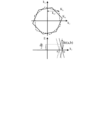
Figure 1: Top, Brillouin zones of two metallic tubes of different helicities. Bottom: Dispersion relation as function of the longitudinal component of the wave vector of the lowest energy bands for these 2 tubes for which $k_{a\parallel}^{0}\neq k_{b\parallel}^{0}$ at the Fermi energy illustrating the second order coupling $\left\langle\Psi_{a}\left|H_{\bot}\right|\Psi_{b}\right\rangle=2t_{\bot}(a,b)^{2}/\delta\epsilon(a,b)$ via the higher energy state at energy $\epsilon_{F}+\delta\epsilon(a,b)/2$ for which $k_{a\parallel}=k_{b\parallel}$.

Going beyond first order perturbation it is possible to show that neighbouring tubes of different helicities are coupled to second order in $H_{\bot}$ with a characteristic energy scale $e_{\bot 2}=2t_{\bot}(a,b)^{2}/\delta\epsilon$ (Fig. 1) involving transitions to higher energy states for which $\epsilon_{b}(k)=\epsilon_{a}(k)=\epsilon_{F}+\delta\epsilon_{(}a,b)/2$. This second order coupling gives rise to an intertube hopping probability which is very small compared to the inverse ballistic time $L/v_{F}$ of a micron long nanotube. It is thus reasonable to assume that, in a rope constituted of tubes of different helicities, electronic transport is confined within each ballistic tube and exhibits a strong 1D character.

II.2 Disordered ropes in the perturbative regime

In the presence of disorder, plane waves localised on individual tubes are perturbed into wave packets and become much more sensitive to the transverse coupling leading to a transport regime which is no longer 1D but can be delocalised on percolating clusters of metallic tubes within the rope.

We consider a very short range (on site) disorder potential, such that its average $<V(x)>=0$ and its variance $\sqrt{<V(x)^{2}>}=W$.

$$V(x)=\sum_{a,x_{a}}W(x_{a})\delta(x-x_{a})$$ (2)

where the index $a$ runs on the chains constituting the rope, each of them being characterized by its atomic sites $x_{a}$ and the the disorder potential $W(x_{a})$ which probability distribution is given by:

$$\begin{array}[]{cccc}P(W(x_{a}))=&1/W&\rm{if}&w(x_{a})\in[-W/2;W/2]\\ &0&\rm{otherwise}&\\ \end{array}$$ (3)

The disorder perturbed wave functions can be written to first order in disorder:

$$|\Psi^{\prime}>=|k_{\bot 0}>\bigg{(}|k_{\parallel 0}>+\sum_{i}\frac{\tilde{V}(k_{\parallel i}-k_{\parallel 0})}{\epsilon(0)-\epsilon(i)}|k_{\parallel i}>\bigg{)}$$ (4)

where i runs over unoccupied states and $\tilde{V}(k)$ is the Fourier component of $V$ at wave vector k. We do not consider transitions involving different values of $k_{\bot}$ and neglect possible perturbation of $t_{\bot}(a,b)$ with disorder.

This perturbed wave function contains plane waves of all values of parallel momentum. As a result electrons can hop from tube to tube and conserve their momentum. The intertube coupling energy between 2 tubes $a$ and $b$ is now $E_{\bot}=<\Psi^{\prime}_{a}|H_{\bot}|\Psi^{\prime}_{b}>$ which reads to first order in the disorder potential:

$$E_{\bot}(a,b)=<k_{a\bot}|H_{\bot}|k_{b\bot}>\frac{2}{L}\sum_{x_{a}}\frac{W(x_{a})\cos((k_{\parallel a}-k_{\parallel b})x_{a})}{\epsilon_{b}(k_{\parallel b})-\epsilon_{b}(k_{\parallel a})}$$ (5)

The disorder average value of this coupling is zero but its typical value $e_{\bot}=\sqrt{\overline{E_{\bot}^{2}}}$ is equal to:

$$e_{\bot}(a,b)=t_{\bot}(a,b)\frac{W}{3\delta\epsilon(a,b)}$$ (6)

with $\delta\epsilon(a,b)=\hbar v_{F}\left|{k_{\parallel a}-k_{\parallel b}}\right|$.

This disorder induced intertube coupling energy is related to the second order coupling term calculated in the previous section through: $e_{\bot}(a,b,W)/e_{\bot 2}(a,b)=W/t_{\bot}(a,b)$ which, as will be shown below, can be much larger than one in a typical rope of SWNT. The coefficients $t_{\bot}(a,b)$ and $\frac{t_{\bot}(a,b)}{\delta\epsilon(a,b)}$ were calculated for all the helicities corresponding to metallic tubes given in table 1 with diameter between 1.2 and 1.5 nm, and are depicted in the histogram fig. (2). From these values we obtain the average value $e_{\bot}=0.03\>W$ .

helicity (n,m)	(9,9)	(10,10)	(11,8)	(12,9)	(12,6)	(13,7)	(15,6)
diameter (nm)	1.24	1.38	1.32	1.45	1.26	1.4	1.5
helicity (n,m)	(14,5)	(13,4)	(16,4)	(15,3)	(17,2)	(16,1)	(18,0)
diameter (nm)	1.36	1.23	1.46	1.33	1.44	1.32	1.43

Table 1: Values of possible helicities and diameters of the 14 metallic tubes with a diameter between 1.5 and 1.2 nm. Diameter and helicity are related through: $D(n,m)=\frac{0.25}{\pi}\sqrt{m^{2}+mn+n^{2}}$. There are also 24 insulating tubes in the same diameter range.

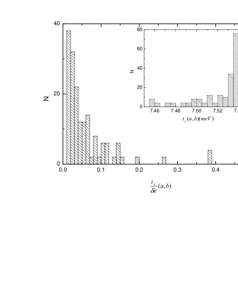
Figure 2: Histogram of possible values of the coefficients $t_{\bot}(a,b)$ and $\frac{t_{\bot}(a,b)}{\Delta\epsilon(a,b)}$ for all couple of helicities $(a,b)$ of metallic tubes with a diameter between 1.2 and 1.5nm. The average yields $3e_{bot}=0.09$.

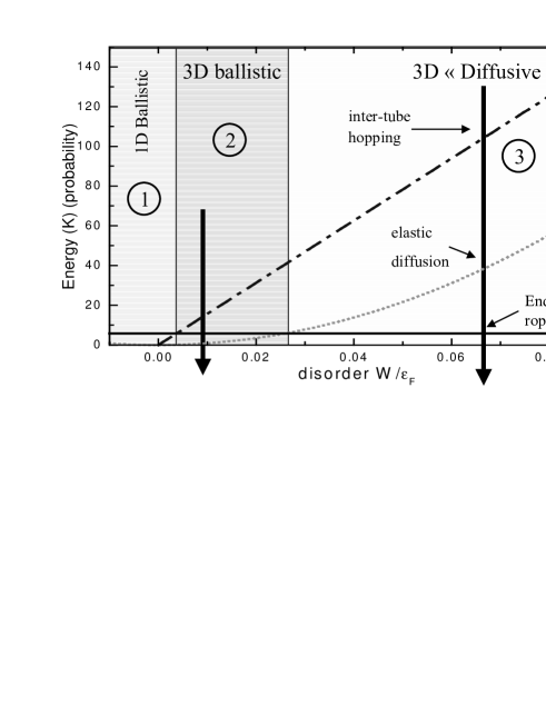
Figure 3: Different transport regimes depending on the amplitude of disorder compared in a rope of length $L=1\mu_{m}$ as discussed in the text. Region 1 $=$ 1D ballistic, region 2 $=$ 3D ballistic and region 3 $=$ 3D diffusive.

To investigate the nature of transport in ropes, it is interesting to compare the typical intertube hopping time $\tau_{h}=\hbar/\left\langle e_{\bot}\right\rangle$ to the intra tube scattering time $\tau_{e}$ induced by the same disorder. The related elastic mean free path $l_{e}=v_{F}\tau_{e}$ was calculated by White et Todorov white98 and found to be given by $l_{e}=\frac{\epsilon^{2}_{F}}{W^{2}}n_{C}$ for a tube of $n_{C}$ carbon atoms along the circumference, where $\epsilon_{F}=2.7\>$eV is the Fermi energy (measured from the bottom of the band) and $W^{2}$ is the variance of the disorder (assumed to be short range). This value of $l_{e}$ is unusually large compared to what is expected in an ordinary conductor, since it is proportional to the number of sites along the circumference of the tube. This is due to the existence of only 2 conduction modes at the Fermi energy regardless of the diameter of the tube. As a result there exists a rather large range of disorder W for which $\tau_{e}$ is greater than $\tau_{h}=\hbar/\left\langle e_{\bot}\right\rangle$, which means that a charge carrier can visit several neighboring tubes between 2 elastic collisions. As shown schematically on fig.3 comparing the relevant time scales for transport in a rope of micron length, four different regimes (1,2,3,4) can be reached as the amplitude of disorder is increased.

1. At very low amplitude of disorder, when both $\tau_{e}$ and $\tau_{h}$ are long compared to the ballistic time $\tau_{b}=L/v_{f}$, transport is ballistic and one dimensional and electronic wave functions are localised within single tubes.

2. When $\tau_{h}<\tau_{b}<\tau_{e}$ transport is still ballistic but wave functions are delocalised over several tubes.

3. When $\tau_{b}<\tau_{h}<\tau_{e}$ transport is diffusive along the percolating clusters of metallic tubes along the rope as long as the rope is shorter than the localisation length which typical value is $\xi=2N_{m}l_{e}$; where $N_{m}$ is the number of metallic tubes in the largest percolating cluster of metallic tubes within the rope. Typical values of $N_{m}$ for commonly investigated SWNT ropes in experiments are given in the appendix.

4. At large disorder $\tau_{b}<\tau_{e}<\tau_{h}$ electronic states are localised within individual tubes at the scale of $l_{e}$ (not shown in fig.3).

From this qualitative model one expects that transverse transport but possibly also longitudinal transport is favored when increasing disorder in the rope. We present in the following section numerical simulations which confirm this statement.

II.3 Analytical results in the localised regime

In the following we consider the case where, in the absence of inter chain coupling, electronic wave functions are localised within each tube aligned along the x axis and can be characterised by the set of parameters $x_{a}$, $k_{a}$ and the localisation length $\xi_{a}$ such that:

$$\begin{array}[]{l}\Psi_{a}(x)=cos(k_{a}(x-x_{a})\exp-(|x-x_{a}|/\xi_{a})/\sqrt{\xi_{a}}=\\ \Sigma_{k=0}^{2n\pi/L}(f_{a}(k-k_{a})+f_{a}(k+k_{a})\exp\left[i((x-x_{a})\right]\end{array}$$ (7)

where $f_{a}$ is a Lorentzian function centered on $k_{a}$ of width $\delta k_{a}=2\pi/\xi_{a}$. In the presence of a small intertube coupling such as described by eq. 12, one can easily compute the typical transverse coupling energy between two nearest neighbor tubes at lowest order in $t_{\perp}$ :

$$\begin{array}[]{l}<\Psi_{a}|H_{\perp}|\Psi_{b}>=\\ \displaystyle\frac{4t_{\perp}(a,b)}{\lambda L}\Sigma_{k}\frac{\exp ik(x_{a}-x_{b})\lambda^{4}}{(\lambda^{2}+(k\pm k_{a})^{2})(\lambda^{2}+(k\pm k_{b})^{2})}\end{array}$$ (8)

In the following we assume that $\delta k_{a}=\delta k_{b}=\lambda=2\pi/\xi$ the summation $\Sigma_{k}$ runs on multiple values of $2\pi/L$ up to $n=L/a_{0}$ the number of sites on the tubes of length $L$. Averaging over the random phase factors $\exp i(k-k^{\prime})(x_{a}-x_{b})$ for $k\neq k^{\prime}$ leads to the average square of this coupling:

$$\begin{array}[]{l}\Gamma_{ab}=|<\Psi_{a}|H_{\perp}|\Psi_{b}>|^{2}=\\ 4t_{\perp}(a,b)^{2}/(\lambda L)^{2}\displaystyle\Sigma_{k}\frac{\lambda^{8}}{\left[\lambda^{2}+((k\pm k_{a})^{2}\right]^{2}\left[\lambda^{2}+((k\pm k_{b})^{2}\right]^{2}}\end{array}$$ (9)

Keeping in the summation over $k$ only the $\lambda/(2\pi/L)$ terms centered around $k_{a}$ and $k_{b}$ within $\delta k=\lambda$, finally yields:

$$\Gamma_{ab}=4(t_{\perp}(a,b))^{2}\lambda L\displaystyle\frac{\lambda^{2}}{\pi L^{2}(\lambda^{2}+(k_{a}-k_{b})^{2})^{2}}$$ (10)

$\lambda$, the inverse typical localisation length for 1D disordered chains can be approximated by $\lambda=Ca_{0}^{-1}W^{2}/E_{F}^{2}$ where the amplitude W of the intra chain on site disorder is assumed to be small compared to the Fermi energy $E_{F}$. One can see from expression (10) that the typical transverse coupling between tubes of different helicities $k_{a}\neq k_{b}$ obtained after averaging on the positions $x_{a}$ and $x_{b}$ increases with disorder like $W^{6}$ at low disorder and decreases like $1/W^{2}$ at large disorder such that $\lambda>|k_{a}-k_{b}|$.

III A simplified anisotropic tight binding model for a rope of SWNT.

We investigate in the following a simplified tight binding model for the transport in a rope containing a percolating cluster of $N_{m}$ metallic SWNT. As shown in the appendix, we expect that in commonly investigated SWNT ropes $N_{m}$ is at most equal to 10. Each SWNT labeled $n$ is described by a simple 1D atomic chain of $N_{s}$ sites with a nearest neighbor coupling energy along the chain $t_{n}$ which can be different from one chain to the other. The variables $t_{n}$ are randomly distributed around their average value $t_{\parallel}$ with a square distribution of width $\delta t_{\parallel}$. For convenience we take the chains on the surface of a cylinder where only sites belonging to nearest neighbor chains are coupled (see Fig.4). This crudely reproduces the situation of a hexagonally packed rope, where each metallic tube has on average 2 metallic tubes as nearest neighbors. The interchain transverse coupling is described by a transverse nearest neighbor coupling $t_{\perp}\ll t_{\parallel}$. The distribution among the $t_{n}$ plays the same role as the helicity distribution among the tubes in a rope i.e. the inter chain coupling becomes zero to first order in $t_{\perp}$ since identical longitudinal Bloch wave vectors correspond to different energies $t_{n}\cos ka_{0}$, except at half filling $ka_{0}=\pi/2$. Note however that this disorder among the $t_{n}$ also implies a distribution of Fermi velocities which does not exist in CNT. This leads to the following hamiltonian $H=H_{\parallel}+H_{\perp}$.

$$H_{\parallel}=\sum_{n=1}^{N_{m}}\sum_{n_{s}=1}^{N_{s}-1}t_{n}\left[|n,n_{s}><n,n_{s}+1|+h.c.\right]$$ (11)

$$\begin{array}[]{l}H_{\perp}=t_{\perp}\sum_{n_{s}=1}^{N_{s}}{\large[}\sum_{n=1}^{N_{m}-1}|n,n_{s}><n+1,n_{s}|+\\ \exp(i\phi)|N_{m},n_{s}><1,n_{s}|+h.c.{\large]}\end{array}$$ (12)

The last term in $H_{\perp}$ corresponds to the periodic boundary conditions around the cylinder modeling the rope. This periodic boundary condition involves a phase factor $\exp(i\phi)$ equivalent to a fictitious flux $\Phi$ through the cylinder which modifies the phase $\phi=2\pi\Phi/\Phi_{0}$ of transverse boundary conditions of the wave functions imry . Due to the different values of $t_{n}$ the wave functions are localised within each chain in the limit of very long chains $N_{s}\gg N_{m}$ and $t_{\perp}\ll t_{\parallel}$. An extra disorder hamiltonian $H_{d}$ is added either as a random distribution of on-site potentials $w_{i}$ of width $W$ or as an extra random contribution $\delta t_{n}(s,s+1)$ to the nearest neighbor coupling $t_{n}$ within the chain $n$ (bond disorder) characterized by a distribution of width $\delta t_{w}$ assumed to be independent of n.

III.1 Numerical results.

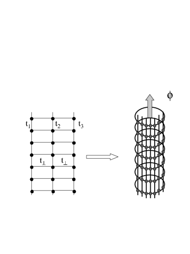
Figure 4: Left: Schematic modelisation of a rope of nanotubes by $N_{m}$ slightly coupled tight binding chains of different longitudinal energies $t_{1}\neq t_{2}\neq t_{3}$ etc…. Right: The chains lye on a cylinder threaded by a fictitious Aharonov Bohm flux which enables to investigate transverse transport.

In order to investigate the interchain localisation and the effect of disorder along the chains, we have calculated the eigenvalues of $H(\phi)=H_{0}(\phi)+H_{d}$. As shown in the seminal work of Thouless thouless72 the sensitivity of these eigenvalues to a change of the phase $\phi$ of the boundary conditions can be considered as a measure of the delocalisation of the wave functions on the various chains constituting the rope. More precisely we have computed the quantity $\delta\epsilon_{perp}=<|\epsilon_{k}(\phi=\pi)-\epsilon_{k}(0)|>_{k}$ where the average $<>_{k}$ is taken on the $N_{m}N_{s}/4$ energy levels of the spectrum between 1/8 and 7/8 filling excluding the region between 3/8 and 5/8 filling. Around half filling the tight binding dispersion relations for all chains are indeed crossing each other whatever the values of $t_{n}$ are and the model is inadequate. For ropes of $N_{m}=10$ chains of $N_{s}=100$ sites the phase dependent eigenvalues were determined using a standard matlab diagonalisation routine. On the other hand for longer ropes ($N_{s}=1000$) a Lancsos algorithm lancsos was used to compute the eigenvalues spectrum. The quantity $\delta\epsilon_{perp}$ calculated for ropes of ten tubes is shown on Fig.5 as a function of disorder strength both for on site and bond disorder.

When the $t_{n}$ are all equal ($\delta t_{\parallel}=0$), $\delta\epsilon_{perp}$ is a monotonously decreasing function of disorder as expected in the physics of standard localisation. On the other hand when the $t_{n}$ are different, $\delta\epsilon_{perp}$ is very small at low values of disorder as expected, with a power law dependence in $t_{\perp}^{10}$ (this exponent corresponds to the hopping probability around a circumference with 10 sites), see Fig.6. More important, at fixed value of $t_{\perp}$, $\delta\epsilon_{perp}$ increases with disorder amplitude, goes through a maximum and decreases at large disorder.

Figure 5: Transverse delocalisation by disorder: Evolution of $\delta\epsilon_{perp}$ with the amplitude of disorder for 10 coupled chains of 100 sites, corresponding to W for on site disorder, and $\delta t_{w}$ for bond disorder. The situation of identical values of $t_{n}$ corresponding to $\delta t_{\parallel}=0$ exhibits expected disorder induced localisation, whereas the situation with different values of $t_{n}$ where $\delta t_{\parallel}/t_{\parallel}=0.2$ shows a regime of disorder induced transverse delocalisation . The transverse hopping energy is chosen to be $t_{\perp}=0.06t_{\parallel}$. $\nu$ is the density of states (inverse nearest level spacing).

As shown in Fig.6 the conditions of observation of this non monotonous dependence of $\delta\epsilon_{perp}$ as a function of disorder amplitude depends drastically on the amplitude of the transverse hopping integral. It is clearly observed for very small values of $t_{\perp}$ with a low disorder increase in $W^{2.5\pm 0.5}$ followed by a decrease in $1/W^{9\pm 1}$. This power law exponent is consistent with the analytical result derived in previous section for the quantity $\Gamma_{ab}^{1/2}\propto 1/W$ describing the large disorder hoping between two adjacent tubes, its extension to hopping processes around a rope containing $N_{m}$ chains yielding a decrease in $1/W^{(}N_{m})$. When increasing $t_{\perp}$ multiple order hopping processes in $t_{\perp}^{10}$ dominate the transverse transport and $\delta\epsilon_{perp}$ becomes independent of disorder at low value of $W$ .

The sensitivity to a phase shift along the chain direction was also investigated from the computation $\delta\epsilon_{par}=<|\epsilon_{k}(\phi_{\parallel}=\pi)-\epsilon_{k}(0)|>_{k}$ where $\phi_{\parallel}$ is the phase factor on periodic boundary conditions parallel to the tube axis. For long ropes (1000 sites along the longitudinal axis) it is possible to observe an increase of $\delta\epsilon_{par}$ with $t_{\perp}$, see Fig. 7. This behavior is associated with an increase of the longitudinal localisation length with $t_{\perp}$ in the range of disorder where the inter tube coupling increases with disorder. One can easily deduce from this figure that for the value of $W=1.3$ the localisation length $\xi(t_{\bot})$ increases by approximatively a factor 4 at $t_{\bot}/t_{\parallel}=0.06$. This is done assuming an $\exp(-L/\xi(t_{\bot}))$ behavior for $\delta\epsilon_{par}$.

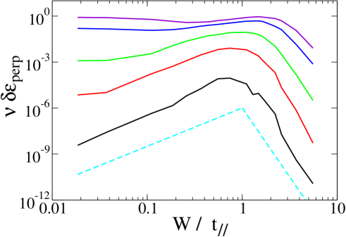
Figure 6: Results obtained by diagonalisation of a system of $N_{m}=10$ chains of $N_{s}=1013$ sites. Continuous curves, average energy difference $\delta\epsilon_{perp}$ as a function of on site disorder amplitude. From top to bottom: $t_{\perp}/t_{\parallel}=0.1,0.07,0.03,0.02,0.01$. Note the dependence in $t_{\perp}^{1}0$ at low disorder. Dashed curve power law fits approximation those curves with $2.5$ and $-9$ exponents (left and right part).

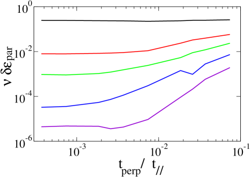
Figure 7: Results obtained by diagonalisation of a system of $N_{m}=10$ chains of $N_{s}=1013$ sites. Average typical energy difference $\delta\epsilon_{par}$ between the symmetric/antisymmetric boundary conditions in the longitudinal direction as a function of $t_{\perp}/t_{\parallel}$. From top to bottom $W/t_{\parallel}=0.55,0.9,1.1,1.3,1.5$

IV Conclusion: implication for the transport in ropes on carbon nanotubes.

We have shown that a rope of single wall carbon nanotubes of different helicities is expected to exhibit very different regimes of electronic transport depending on the amount of disorder. When disorder is very small electronic transport takes place in independent 1D ballistic tubes. The conductance is then expected to be $G=2NG_{Q}$ where N is the number of connected metallic tubes. The experimental observation of a strong shot noise reduction in short low resistive ropes roche02 confirms the ballistic nature of transport in these ropes. On the other hand disordered tubes are expected to behave as 3D diffusive multi channel conductors whose maximum value of conductance is $G=2N_{m}(l_{e}/L)G_{Q}$ when L is smaller than the localization length $\xi=2N_{m}l_{e}$, where $N_{m}$ is the number of metallic tubes in the largest percolating cluster of metallic tubes in the rope. Four probe transport measurements on NT ropes after ion irradiation damage avouris00 have been shown to give information on the intertube hopping processes within the rope which was found to increase with disorder. These findings can also be interpreted taking into account the increase of the intertube scattering rate with disorder. The physics of intertube transfer has also been shown to play an important role in the transport in multiwall nanotubes bourlon04 ; revueNTcharlier07 . The situation is however different than in ropes since each tube is only coupled within first order to two other tubes (nearest inner and outer shells) and moreover only the most external tube is connected to electrodes.

Let us also mention that a similar scenario of disorder induced delocalisation has been predicted to take place in networks of disordered polymers as discussed in prigodin93 ; zambetaki96 ; dupuis97 .

We finally note that these different types of transport are also expected to influence the superconductivity observed at very low temperature on ropes of carbon nanotubes. The superconductivity in weakly disordered ropes has been observed to exhibit a strongly 1D character with a T=0, H=0 transition. On the other hand more resistive ropes exhibit a broad transition at finite temperature characteristic of a multi channel quasi 3D system kociak01 ; kasumov03 .

Acknowledgments: We acknowledge very fruitful discussions with Christophe Texier, Nicolas Dupuis, Michael Feigelmann, Piotr Chudzinski and Alexei Ioselevitch on this problem.

V Appendix: Determination of the typical size of percolating cluster of metallic tubes within a rope.

Carbon nanotubes in a rope are arranged according to a triangular network, with on average 1/3 of metallic tubes and 2/3 of semiconducting ones. Since 1/3 is below the percolating threshold, 1/2, for nearest neighbor couplings in the 2D triangular lattice, the metallic tubes do not percolate over the full rope and constitute disconnected clusters which size distribution depends on the number of tubes within the rope. We have calculated numerically this size distribution for ropes containing a few hundred tubes. This result is shown on Fig.8 for ropes containing 100 and 400 tubes. The size distribution decays exponentially with the number of tubes in a cluster. We find that for a rope containing 400 tubes the average cluster size is 3 but by integrating the number of clusters of size above a given value we find that there is at least one cluster of tubes of size above 15.

Figure 8: Size distribution of the number of tubes n in a percolating cluster of metallic tubes for ropes containing N=100 and N=400 tubes among which 1/3 on average are metallic.

References

- (1) M. Dresselhaus, G. Dresselhaus, and P. Eklund, Science of Fullerenes and Carbon Nanotubes, Academic Press, San Diego, CA, 1996.
- (2) C. Journet, W. Maser, P. Bernier, A. Loiseau, M. L. de la Chapelle, S. Lefrant, P. Deniard, R. Lee, and J. Fisher, Nature 388, 756 (1997).
- (3) A. Maarouf, C. Kane, and E. Mele, Phys. Rev. B 61(16), 11156 (2000).
- (4) M.A. Tunney and N.R.Cooper Phys. Rev. B 74(16), 075406 (2006).
- (5) P. E. Roche, M. Kociak, S. Guéron, A. Kasumov, B. Reulet, and H. Bouchiat, Very Low Shot Noise in Carbon Nanotubes, Eur. Phys. J. B 28, 217 (2002).
- (6)
- (7) J. T. Edwards and D. J. Thouless, Numerical Studies of Localization in Disordered Systems, J. Phys. C: Solid State Phys 5, 807 (1972).
- (8) C. Lanczos, J.Res. Nat. Bur. Standards, Sec. B 45, 225 (1950).
- (9) C. T. White and T. N. Todorov, Carbon Nanotubes as Long Ballistic Conductors, Nature 393, 240 (1998).
- (10) H. Stahl, J. Appenzeller, R. Martel, Ph. Avouris, and B. Lengeler 85,5186(2000).
- (11) J.C. Charlier, X. Blase, and S. Roche Rev. Mod. Phys., 79, 677 (2007).
- (12) B. Bourlon, C. Miko, L. Forr , D. C. Glattli, and A. Bachtold Phys. Rev. Lett. 93, 176806 (2004).
- (13) V. N. Prigodin and K. B. Efetov, Localization Transition in a Random Network of Metallic Wires: A Model for Highly Conducting Polymers, Phys. Rev. Lett 70, 2932 (1993).
- (14) I. Zambetaki, S. N. Evangelou, and E. N. Economou, The Anderson Transition in a Model of Coupled Random Polymer Chains, J. Phys.: Condens. Matter 8, 605 (1996).
- (15) N. Dupuis, Metal-Insulator Transition in Highly Conducting Oriented Polymers, Phys. Rev. B 56, 3086 (1997).
- (16) M. Kociak, A. Kasumov, S. Guéron, B. Reulet, I. I. Khodos, Y. B. Gorbatov, V. T. Volkov, L. Vaccarini, and H. Bouchiat, Phys. Rev. Lett. 86(11), 2416 (2001).
- (17) A. Kasumov, M. Kociak, M. Ferrier, R. Deblock, S. Guéron, B. Reulet, I. Khodos, O. Stéphan, and H. Bouchiat, Quantum Transport Through Carbon Nanotubes: Proximity-Induced and Intrinsic Superconductivity, Phys. Rev. B 68, 214521 (2003).