Statistics of harmonic measure and winding of critical curves from conformal field theory

Abstract

Fractal geometry of random curves appearing in the scaling limit of critical two-dimensional statistical systems is characterized by their harmonic measure and winding angle. The former is the measure of the jaggedness of the curves while the latter quantifies their tendency to form logarithmic spirals. We show how these characteristics are related to local operators of conformal field theory and how they can be computed using conformal invariance of critical systems with central charge $c\leqslant 1$.

1 Introduction

Geometric properties of critical two-dimensional systems of statistical mechanics have attracted considerable interest of both physicists and mathematicians in recent years. On the one hand, methods of quantum gravity have been successfully applied by Duplantier to obtain the multifractal spectrum of harmonic measure on critical cluster boundaries [1, 2]. On the other hand, the invention of the Schramm-Loewner evolution (SLE) by Schramm [3] has made it possible to study conformally-invariant critical curves rigorously (several reviews of SLE are available by now; see, for example, Refs. [4, 5, 6, 7, 8]).

Conformal field theory (CFT ) has been a natural and traditional language for description of critical statistical systems in two dimensions. It is important to understand how fractal properties of critical curves can be obtained from CFT. A part of the emerging picture is that the stochastic geometry of critical curves can be studied by traditional methods of CFT. As any local field theory, CFT focuses on correlation functions of local operators. It turns out that the stochastic geometry of critical curves is related to correlators of certain primary fields in CFT. This connection, first discussed in Ref. [9], has been further developed in our papers [10, 11] where we have identified the curve-creating primary operators and considered their correlators with other primaries serving as “probes” of harmonic measure. Along this way we have reproduced Duplantier’s results for multifractal exponents associated with harmonic measure.

In addition to harmonic measure, complicated planar domains and their boundaries are characterized by winding or rotation. The notion of rotation spectrum for planar domains has been introduced by Binder in Ref. [12]. Then the mixed rotation and harmonic measure spectrum has been found exactly for critical curves by Duplantier and Binder [13]. In that paper the authors combined an earlier Coulomb gas approach to the distribution of winding angles of critical curves [14] with the quantum gravity methods of Refs. [1, 2].

In this paper we extend our previous analysis [10, 11] to include the winding (rotation) of critical curves. As it happens, to account for rotation of critical curves, we need to consider CFT primary fields with complex weights and charges. The procedure involves an analytic continuation of chiral correlation functions and then gluing the chiral sectors to obtain real but angular dependent correlators. The paper is organized as follows. In Section 2 we formulate the problem and give heuristic definitions of various objects of interest including harmonic measure and rotation of critical curves. In Section 3 we consider a special case of a single probe of harmonic measure and rotation near a star configuration of several critical curves. Then we go on to the general case, where several probes can be placed in the vicinity of a critical star configuration. We conclude in Section 5 with a discussion and comparison with other works.

2 Description of the problem

Consider a two-dimensional critical statistical system. Such systems can be formulated as critical points in an ensemble of curves on a lattice, e.g. the loops of the $O(n)$ model or the high-$T$ expansion loops of the $Q$-state Potts model. When the system is critical, these curves are called critical curves. In the continuum limit, statistical systems are invariant under conformal transformations and can be described by a CFT with a certain central charge $c$. In this case the critical curves are fluctuating fractal curves.

Any conformal transformation in two dimensions locally looks like a combination of rotation and a scale transformation (dilatation). For a given composition of dilatation and rotation in the plane there exist curves which remain invariant. They are logarithmic spirals $\phi=\lambda\ln r$. The quantity $\lambda$ characterizes the winding of a spiral and is called the rate of rotation. For a pure dilatation the spirals degenerate into straight lines (no rotation: $\lambda=0$) which may intersect and form corners with arbitrary opening angles.

Since any conformal transformation is locally a composition of dilatation and rotation, a conformally invariant critical curve can be thought of as an assembly of elementary corners and logarithmic spirals at all scales. The so called multifractal analysis aims at determining the fractal dimensions of the subsets of a critical curve with given opening angle and winding. These fractal dimensions form a continuous family of multifractal exponents.

Harmonic measure is another way of characterizing the complicated fractal geometry of a critical curve. In a simple electrostatic analogy we can imagine that a critical cluster is charged with a unit charge that all goes to the boundary of the cluster. Charge density (which is the density of harmonic measure) on the boundary is very uneven and lumpy, and can be characterized by its moments. Therefore, in the ensemble of critical curves it is natural to characterize their fractal geometry by the statistics of local winding and harmonic measure near some point on the curve.

Locally, near a charged corner the scaling of the charge density or, equivalently, of the magnitude of the electric field $E$ is determined by the opening angle $\beta$ at the corner: $rE(r)\sim r^{\pi/\beta}$. What will be important for us in the following is that this power-law behavior is the same along all straight lines that converge at the apex of the corner. All these lines intersect the equipotentials at constant angles $\theta$, and only one of them is an electric field line (corresponding to $\theta=\pi/2$). In mathematics such lines are sometimes called “slanted Green lines”, while the electric field lines are called “Green lines”. In a general situation we will denote the slanted Green line that goes from the origin and forms the angle $\theta$ with equipotentials by $\gamma_{\theta}$.

Similar statements can be made for a logarithmic spiral. The information about the rate of rotation $\lambda$ of a spiral is contained in the winding of any of the slanted Green lines that emanate from the spiral’s origin. It is easy to see that the line $\gamma_{\theta}$ is the rotated logarithmic spiral $\phi=2\theta+\lambda\ln r$ (with $\theta=\pi/2$ again corresponding to the unique electric field line going from the origin), and we can follow any of them to “measure” $\lambda$.

The information on the scaling of the magnitude of the electric field and the winding of a slanted Green line near a certain point on the critical curve is contained in the value of the derivative of a uniformizing conformal map $w(z)$ that maps the exterior of the critical cluster onto a standard simple domain. In these terms, the electrostatic potential of the curve is $-\log|w(z)|$, the magnitude of the field near the curve is $E=|w^{\prime}(z)|$, and the direction of the field is related to $\arg w^{\prime}(z)$. (In terms of the complex potential $\Phi(z)=-\log w(z)$ we have $\Phi^{\prime}(z)=-E_{x}+iE_{y}$.) We will use this idea extensively in what follows. It is convenient for our purposes to restrict the statistical ensemble so that a critical curve always passes through a fixed point, and work in the vicinity of this point.

In this paper we consider only dilute critical systems, which means that critical curves generically do not intersect (see, however, the discussion of exceptional star configurations below). This choice is dictated by the nature of our problem. In the dense phase where critical curves have multiple points, the harmonic measure is only supported on the external perimeters of critical clusters (think of electric charge spreading on the surface of a conductor). The external perimeters are always simple critical curves described by a model in the dilute phase, and it is sufficient to consider dilute systems in our problem. The prime example of this phenomenon is provided by critical percolation: percolation hulls intersect themselves at all scales, while the external perimeters of percolation clusters are simple curves in the universality class of self-avoiding random walks.

In the absence of boundaries in the system critical curves are closed loops. If the system has a boundary and the boundary condition changes at certain boundary points, it gives rise to critical curves which start and end at these points. A hole in the system is a component of the boundary. If the boundary condition changes on it, we will observe critical curves emanating from the hole. On scales much larger than the size of the hole the latter becomes a puncture. In this case there are critical curves coming out of a single point in the bulk of the system. Inserting a puncture at some point in the bulk we can ensure that in each realization of the statistical ensemble there is a “star” — a fixed number $k$ of curves starting from this point.

Generally speaking, a critical system need not contain punctures or be restricted in any way by insertion of curve-creating operators. These are merely artificial devices which we will use in our calculations. The meaning of $k=2$ stars is obvious: any point on a curve is such a star. In fact, stars with $k>2$ can also be meaningful even in the absence of punctures. A star with an even number $k\geqslant 4$ of legs is a point of self-intersection of a critical curve. Since in the dilute phase the latter are simple curves with probability one, stars with $k\geqslant 4$ can only appear as exceptional configurations in rare realizations of the statistical ensemble, all such realizations having the total weight (probability) zero. In fact, we can quantify this discussion by assigning a negative fractal dimension $d_{k}$ (see Eq. (50) below) to the set of stars with $k\geqslant 4$ legs. The meaning of a negative fractal dimension is as follows. If in a system of size $L$ several curves approach each other within a distance $l$, then on the scales much larger than $l$ the configuration of the curves will look like a star. However, in a typical realization of the statistical ensemble, the number of points where such approach happens, scales as $(L/l)^{d_{k}}$, and goes to zero in the thermodynamic limit.

In the rest of the paper we apply methods of CFT to the problem of the mixed multifractal spectrum of harmonic measure and winding of critical curves. In this approach a $k$-legged star of critical curves is created by an insertion of a specific curve-creating operator $\psi_{0,k/2}$ [9, 10, 11]. This operator can be realized as a vertex operator in the Coulomb gas formulation of CFT, and has known holomorphic charge $\alpha_{0,k/2}$ and weight $h_{0,k/2}$, see Eqs. (4, 5, 6) below. Other primary operators inserted close to the curve-creating one can then serve as probes for the harmonic measure. This has been explained and used in our previous works [10, 11]. In the present paper we will see that to account for winding of critical curves, the probes must have complex charges and conformal weights.

We want to point out here that while harmonic measure can behave nontrivially and be probed both in the bulk and on a boundary of a critical system, the mixed spectrum that takes into account winding is only defined in the bulk. Indeed, there is no way a critical curve can rotate around a point on a boundary. Therefore, our present analysis only deals with the bulk curve creating operators.

3 The case of a single point

For simplicity we start with the case of the electric field (both the magnitude and the direction) measured at a single point and then generalize the method to multiple points.

3.1 Definition of multifractal exponents

Consider a $k$-legged star — $k$ critical curves emanating from the origin in the bulk of the system. We are interested in the properties of the star much closer to the origin than the system boundaries. The shape of the legs of the star far from the origin is unimportant, which allows us to trace each leg only up to a certain distance from the origin. Let us describe the shape of such a truncated star by an analytic function $w(z)$ which maps the exterior $\mathbb{S}$ of the star onto the exterior of the unit disk $\mathbb{C}\backslash\mathbb{D}$. The statistical ensemble of the shapes of the star defines the statistical ensemble of $w(z)$.

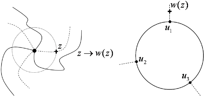
Figure 1: The conformal transformation blows up the star into the shape of a disk, like a puffer fish. The origin of the star is mapped to several points $u_{i}$. The point $z$ is chosen to lie on the dotted circle of a fixed radius and so that $w(z)$ lies on the same radial line as $u_{1}$.

Close to the origin the $k$ curves of the star divide the plane into $k$ sectors. Approached from different sectors, the origin is mapped onto $k$ points $u_{i}$ on the unit circle: $\lim_{z\to 0}w(z)=u_{i}$ for $z$ in the $i$-th sector. To make $w(z)$ unique we specify $w(\infty)=\infty$ and $w^{\prime}(\infty)=\rho^{-1}>0$, where $\rho$ is the conformal radius of the star. Its fluctuations are unimportant. For each realization of the star we can choose the truncation radius so that $\rho=1$.

As we have explained above, the magnitude and the direction of the electric field at a point $z$ are determined by $|w^{\prime}(z)|$ and $\arg w^{\prime}(z)$ respectively. Both these quantities are random. Conformal invariance suggests that locally $|w^{\prime}(z)|$ scales as a power of $|z|$ and $\arg w^{\prime}(z)$ behaves as $\lambda\ln|z|$. Therefore, we can study the joint moments of $|w^{\prime}(z)|$ and $e^{\arg w^{\prime}(z)}$ expecting them to scale as

$$\mathbf{E}\big{[}|w^{\prime}(z)|^{n}e^{p\arg w^{\prime}(z)}\big{]} \sim|z|^{\Delta_{k}(n,p)},$$ (1)

where $\mathbf{E}$ denotes average over the fluctuating geometry of the star. This equation defines the multifractal exponents $\Delta_{k}(n,p)$, and our goal below is to obtain them using methods of CFT.

Let us now discuss a subtle point about Eq. (1). We can treat the average over the star shapes in two ways. The first way is to specify the position of point $z$ in such a way that for any star $\mathbb{S}$ this point is on the slanted Green line $\gamma_{\theta}$ in, say, the first sector (the choice of the sector is arbitrary and immaterial). Let us denote this choice by $z_{\theta}$ (implicitly keeping in mind that the choice depends on the star shape). Then the average in the left hand side of Eq. (1) should be understood as

$$\mathbf{E}\big{[}|w^{\prime}(z_{\theta})|^{n}e^{p\arg w^{\prime}(z_{\theta})}\big{]} \sim|z_{\theta}|^{\Delta_{k}(n,p)},$$ (2)

(only the argument of $z_{\theta}$ fluctuates here, while $|z_{\theta}|$ is fixed). The simplest such choice is to place $z$ on the electric field line $\gamma_{\pi/2}$. Then in the $w$ plane the image $w(z)$ lies on a radial straight line:

$$\arg w(z_{\pi/2})=\arg u_{1},$$ (3)

see Fig. 1 for illustration.

On the other hand, as we have argued in the previous section, the scaling of $|w^{\prime}(z)|$ and $e^{\arg w^{\prime}(z)}$ should be the same along any line $\gamma_{\theta}$. Therefore, we can average (integrate) over $\theta$ (and sum over the different sectors) in Eq. (2) while keeping $|z_{\theta}|$ constant. This procedure produces a manifestly rotationally invariant average. In this average we can distribute the contributions that come from star shapes which differ by a global rotation around the origin into sets, and then sum up all such sets. Due to isotropy of our critical system, all terms in a given set have the same statistical weight. Therefore, to calculate the average, we can choose any single term from each set and sum these up. We can choose these terms so that $\arg z$ is the same for all of them, which gives the left hand side in Eq. (1) with a fixed point $z$. This is the second way to interpret the average over the star shapes. As we see, the two ways are equivalent and produce the same scaling behavior with the multifractal exponents $\Delta_{k}(n,p)$.

3.2 CFT calculation of multifractal exponents

A critical system is characterized by the central charge $c$ which we parametrize, as is usual in CFT, by the so called background charge $\alpha_{0}$:

$$c =1-24\alpha_{0}^{2}.$$ (4)

As we have shown in Ref. [11], in the Coulomb gas description of the dilute phase we have to impose the Dirichlet conditions on the system boundaries. A consistent way of doing it also implies that the background charge $\alpha_{0}$ in Eq. (4) is non-positive: $\alpha_{0}\leqslant 0$.

Within the CFT description (see [11, 16] for introduction to the mathematical apparatus of CFT used below) a $k$-legged star centered at the origin is created by inserting the curve-creating operator $\psi_{0,k/2}(0)$ [10, 11]. This operator has holomorphic charge

$$\alpha_{0,k/2}=\alpha_{0}-\frac{k}{4}\big{(}\alpha_{0}-\textstyle\sqrt{\alpha_{0}^{2}+1}\big{)},$$ (5)

and its antiholomorphic charge is $\bar{\alpha}_{0,k/2}=-\alpha_{0,k/2}$. It is spinless with real conformal weights:

$$h=\bar{h}=h_{0,k/2}=\alpha_{0,k/2}(\alpha_{0,k/2}-2\alpha_{0}).$$ (6)

To calculate the mixed multifractal exponents $\Delta_{k}(n,p)$ by means of CFT we consider a primary operator $\mathcal{O}_{h,\bar{h}}$ whose holomorphic and antiholomorphic weights $h,\bar{h}$ are complex and conjugate to each other:

$$\bar{h}=h^{*}.$$ (7)

(Notice that we use asterisk to denote complex conjugation, while the bar over a weight or charge simply indicates the antiholomorphic sector.) Its holomorphic and antiholomorphic charges are related to the weights by the equations [11]

$$h =\alpha(\alpha-2\alpha_{0}), \bar{h} =\bar{\alpha}(\bar{\alpha}+2\alpha_{0}).$$ (8)

(The introduction of the charges is convenient because they make fusion of primary operators look simple: the charges of the fused fields simply add up.) Note the sign difference in the formula for $\bar{h}$ compared to that in Ref. [16]. The difference is necessitated by our convention ($\alpha_{0}\leqslant 0$) for the dilute phase. The solutions $\alpha(h)$, $\bar{\alpha}(\bar{h})$ are chosen so that $\alpha(0)=\bar{\alpha}(0)=0$:

$$\alpha =\alpha_{0}+\scriptstyle{\sqrt{\textstyle\alpha_{0}^{2}+h}}, \bar{\alpha} =-\alpha_{0}-\scriptstyle{\sqrt{\textstyle\alpha_{0}^{2}+\bar{h}}}.$$ (9)

The two charges are related by $\bar{\alpha}=-\alpha^{*}$. If we denote the real and imaginary parts of the holomorphic charge as $\alpha^{\prime}$ and $\alpha^{\prime\prime}$, the real and imaginary parts of the holomorphic weight $h$ can be written as

$$\text{Re}\,h =\alpha^{\prime 2}-\alpha^{\prime\prime 2}-2\alpha_{0}\alpha^{\prime}, \text{Im}\,h =2\alpha^{\prime\prime}(\alpha^{\prime}-\alpha_{0}).$$ (10)

The operator $\mathcal{O}_{h,\bar{h}}$ plays the role of a “probe” of harmonic measure and rotation of critical curves when we place it at a point $z$ near the origin of a $k$-star. The star is created by inserting the curve-creating operator $\psi_{0,k/2}(0)$. Thus we propose to consider the following correlation function:

$$\Big{\langle}\psi_{0,k/2}(0)\mathcal{O}_{h,\bar{h}}(z)\Psi(\infty)\Big{\rangle}\propto\big{|}z^{2\alpha_{0,k/2}\alpha}\big{|}^{2}=|z|^{4\alpha_{0,k/2}\alpha^{\prime}}e^{-4\alpha_{0,k/2}\alpha^{\prime\prime}\arg z}.$$ (11)

Here and in what follows these angular brackets denote a CFT average and $\Psi$ stands for all operators far from the origin and is necessary to make the correlation function non-zero. The right hand side in Eq. (11) was obtained in a standard way by fusion of primary operators (expressed as vertex operators in the Coulomb gas formulation of CFT). Notice that the presence of complex weights and charges leads to an expression that is explicitly angular dependent and multivalued. Thus, this correlator does not correspond to any physical quantity, and we need to consider

$$C=\Big{\langle}e^{4\alpha_{0,k/2}\alpha^{\prime\prime}\arg z}\psi_{0,k/2}(0)\mathcal{O}_{h,\bar{h}}(z)\Psi(\infty)\Big{\rangle}\propto|z|^{4\alpha_{0,k/2}\alpha^{\prime}}.$$ (12)

In this formulation the position of the point $z$ is fixed, and the extra exponential factor is a constant that can be pulled out of the average $\langle\ldots\rangle$.

The same correlation function $C$, being an average over all degrees of freedom in the system, can be evaluated in another way, using the so-called two-step averaging procedure [7, 10, 11, 15]. We can first fix the shape of the star and sum over the rest of the degrees of freedom. Then we average over all possible shapes of the star:

$$C=\mathbf{E}\Big{[}e^{4\alpha_{0,k/2}\alpha^{\prime\prime}\arg z}\big{\langle}\mathcal{O}_{h,\bar{h}}(z)\Psi(\infty)\big{\rangle}_{\mathbb{S}}\Big{]}.$$ (13)

The subscript of a correlation function refers to the domain in which it is computed, in this case the exterior of the star $\mathbb{S}$.

The point $z$ is still fixed in Eq. (13), therefore, for each shape $\mathbb{S}$ this point lies on a different slanted Green line $\gamma_{\theta}$. However, as in Section 3.1, we can argue that the scaling with $|z|$ is the same (independent of $\theta$) for all the terms with different values of $\theta$. Then to find the exponents $\Delta_{k}(n,p)$ it is sufficient to retain only terms with a fixed (in each star configuration) value of $\theta$ and consider a different quantity

$$C_{\theta}=\mathbf{E}\Big{[}e^{4\alpha_{0,k/2}\alpha^{\prime\prime}\arg z_{\theta}}\big{\langle}\mathcal{O}_{h,\bar{h}}(z_{\theta})\Psi(\infty)\big{\rangle}_{\mathbb{S}}\Big{]}.$$ (14)

There is a parallel between the correlator $C$ and the expression in Eq. (1), and the correlator $C_{\theta}$ and the expression in Eq. (2): though $C$ and $C_{\theta}$ are formally very different objects, they scale with $|z|$ in the same way. The crucial difference between $C$ and $C_{\theta}$ is that in the latter object the argument of $z_{\theta}$ is fluctuating (it depends on the star configuration) and the factor $e^{4\alpha_{0,k/2}\alpha^{\prime\prime}\arg z_{\theta}}$ must be kept under the average $\mathbf{E}[\ldots]$.

The next step in transforming the expression (14) is to map the exterior of the star $\mathbb{S}$ onto the exterior of the unit disk by $w(z)$. Under this map the operator $\mathcal{O}_{h,\bar{h}}$ transforms according to the definition of a CFT primary field, and operators at infinity do not transform due to the normalization of $w(z)$. Then conformal covariance of correlators of CFT implies

$$C_{\theta}=\mathbf{E}\Big{[}e^{4\alpha_{0,k/2}\alpha^{\prime\prime}\arg z_{\theta}}w^{\prime}(z_{\theta})^{h}\bar{w}^{\prime}(\bar{z}_{\theta})^{\bar{h}}\big{\langle}\mathcal{O}_{h,\bar{h}}(w(z_{\theta}))\Psi(\infty)\big{\rangle}_{\mathbb{C}\backslash\mathbb{D}}\Big{]}.$$ (15)

In this correlator the value of the angle $\theta$ is immaterial. For simplicity of notation let us choose it to be $\theta=\pi/2$, which means that the point $z_{\pi/2}$ is chosen according to Eq. (3) and lies on the unique electric field line connected to the origin of the star. We will drop the subscript $\pi/2$ in the subsequent equations.

In the $w$ plane, $\arg w(z)$ is a fixed number no greater than $2\pi$. At the same time, when $w(z)$ approaches $u_{1}$, its pre-image $z$ moves along the electric field line and exhibits a lot of winding. Since $\arg w(z)\sim\arg w^{\prime}(z)+\arg z$, we can write

$$\arg z\sim-\arg w^{\prime}(z),$$ (16)

because both angles here are large. Thus, we can replace $\arg z$ by $-\arg w^{\prime}(z)$ in Eq. (15). Using Eq. (10) we can also rewrite

$$w^{\prime}(z)^{h}\bar{w}^{\prime}(\bar{z})^{\bar{h}} =\big{|}w^{\prime}(z)^{h}\big{|}^{2}=|w^{\prime}(z)|^{2\,\text{Re}\,h}e^{-2\,\text{Im}\,h\arg w^{\prime}(z)}$$

$$=|w^{\prime}(z)|^{2(\alpha^{\prime 2}-\alpha^{\prime\prime 2}-2\alpha_{0}\alpha^{\prime})}e^{-4\alpha^{\prime\prime}(\alpha^{\prime}-\alpha_{0})\arg w^{\prime}(z)}.$$ (17)

The remaining CFT correlation function in the exterior of the disk is computed by fusion of the primary field with the boundary (which means the fusion of the holomorphic part $\mathcal{O}_{h}(w(z))$ with its image across the boundary of the unit disk). According to Eq. (3), both $w(z)$ and its image in the unit circle $1/w^{*}(z)$ have the same (constant) argument $\arg u_{1}$. Then we find the following scaling behavior:

$$\big{\langle}\mathcal{O}_{h,\bar{h}}(w(z))\Psi(\infty)\big{\rangle}_{\mathbb{C}\backslash\mathbb{D}} \propto\Bigl{(}w(z)-\frac{1}{w^{*}(z)}\Bigr{)}^{-2\alpha\bar{\alpha}}\sim|w(z)-u_{1}|^{2|\alpha|^{2}}$$

$$\sim|z|^{2(\alpha^{\prime 2}+\alpha^{\prime\prime 2})}|w^{\prime}(z)|^{2(\alpha^{\prime 2}+\alpha^{\prime\prime 2})}.$$ (18)

At this stage the correlator $C_{\theta}$ evaluated in two steps becomes

$$C_{\theta} \sim|z|^{2(\alpha^{\prime 2}+\alpha^{\prime\prime 2})}\mathbf{E}\Big{[}|w^{\prime}(z)|^{4\alpha^{\prime}(\alpha^{\prime}-\alpha_{0})}e^{-4\alpha^{\prime\prime}(\alpha^{\prime}-\alpha_{0}+\alpha_{0,k/2})\arg w^{\prime}(z)}\Big{]}.$$ (19)

Since, as we have argued, both $C$ and $C_{\theta}$ should scale in the same way with $|z|$, comparison with Eq. (12) gives

$$\mathbf{E}\Big{[}|w^{\prime}(z)|^{4\alpha^{\prime}(\alpha^{\prime}-\alpha_{0})}e^{-4\alpha^{\prime\prime}(\alpha^{\prime}-\alpha_{0}+\alpha_{0,k/2})\arg w^{\prime}(z)}\Big{]}\sim|z|^{-2(\alpha^{\prime 2}+\alpha^{\prime\prime 2})+4\alpha^{\prime}\alpha_{0,k/2}}.$$ (20)

The last equation is identical to the definition (1) provided we denote

$$n=4\alpha^{\prime}(\alpha^{\prime}-\alpha_{0}),\qquad p=-4\alpha^{\prime\prime}(\alpha^{\prime}-\alpha_{0}+\alpha_{0,k/2}),$$ (21)

$$\Delta_{k}(n,p)=-2(\alpha^{\prime 2}+\alpha^{\prime\prime 2})+4\alpha^{\prime}\alpha_{0,k/2}.$$ (22)

As usual, we need to choose the solutions of Eqs. (21) that vanish for $n=0,p=0$:

$$2\alpha^{\prime} =\alpha_{0}+\textstyle\sqrt{\alpha_{0}^{2}+n}, \alpha^{\prime\prime} =-\frac{p}{4(\alpha^{\prime}-\alpha_{0}+\alpha_{0,k/2})}.$$ (23)

Substituting these values into Eq. (22) we find the mixed multifractal exponents $\Delta_{k}(n,p)$. With the shorthand

$$\alpha_{n}=\alpha_{0}+\textstyle\sqrt{\alpha_{0}^{2}+n}$$ (24)

the answer can be written as

$$\Delta_{k}(n,p)=2\alpha_{0,k/2}\alpha_{n}-\frac{1}{2}\alpha_{n}^{2}-\frac{1}{8}\frac{p^{2}}{\left(\frac{1}{2}\alpha_{n}-\alpha_{0}+\alpha_{0,k/2}\right)^{2}}.$$ (25)

We can also rewrite this result as

$$\Delta_{k}(n,p)=\Delta_{k}(n)-\frac{1}{4}\frac{p^{2}}{\Delta_{k}(n)+n+2(\alpha_{0,k/2}-\alpha_{0})^{2}},$$ (26)

where

$$\Delta_{k}(n)=\Delta_{k}(n,0)=2\alpha_{0,k/2}\alpha_{n}-\frac{1}{2}\alpha_{n}^{2}.$$ (27)

4 The general case

To define a multi-point generalization of the mixed spectrum (1) we consider the following average:

$$\mathbf{E}\Bigl{[}e^{p\arg w^{\prime}(z_{1})}\prod_{i=1}^{k}|w^{\prime}(z_{i})|^{n_{i}}\Bigr{]}\sim r^{\Delta_{k}(\{n_{i}\},p)}.$$ (28)

Here all the points $z_{i}$ have the same distance to the star origin: $|z_{i}|=r$, and no two of them lie in the same sector. Because the curves do not intersect, all the winding angles $\arg w^{\prime}(z_{i})$ differ by no more than $2\pi$, and since they are all very large, they must all scale in the same way: $\arg w^{\prime}(z_{i})\sim\arg w^{\prime}(z_{1})$. Thus, the topology of the star leads to only one parameter $p$ describing the rotation, while we have $k$ parameters $n_{i}$ for harmonic measure in each of the sectors between the star’s legs.

Similar to the discussion in Section 3.1 the points $z_{i}$ can be either fixed or can be chosen to lie on specific slanted Green lines. These choices do not affect the scaling with $r$ in Eq. (28). For example, we can choose $\arg z_{i}$ by the requirement

$$\arg w(z_{i})=\arg u_{i}.$$ (29)

Then in all realizations of the star each $z_{i}$ lies on the unique Green line in the $i$-th sector that starts at the star’s origin.

The calculation of $\Delta_{k}(\{n_{i}\},p)$ is a straightforward generalization of the calculation of the previous section. We introduce $k$ primary operators $\mathcal{O}_{h_{i},\bar{h}_{i}}(z_{i})$ each with complex conjugate weights: $\bar{h}_{i}=h^{*}_{i}$ and holomorphic charges $\alpha_{i}=\alpha^{\prime}_{i}+i\alpha^{\prime\prime}_{i}$. In close parallel to Eq. (12) we consider a CFT correlation function:

$$C_{k} =\Bigl{\langle}e^{4\alpha_{0,k/2}\sum_{i}\alpha_{i}^{\prime\prime}\arg z_{i}+4\sum_{i<j}(\alpha^{\prime}_{i}\alpha^{\prime\prime}_{j}+\alpha^{\prime\prime}_{i}\alpha^{\prime}_{j})\arg(z_{i}-z_{j})}$$

$$\quad\times\psi_{0,k/2}(0)\prod^{k}_{i=1}\mathcal{O}_{h_{i},\bar{h}_{i}}(z_{i})\Psi(\infty)\Bigr{\rangle}.$$ (30)

This correlation function can be computed by fusion of primary fields:

$$\Bigl{\langle}\psi_{0,k/2}(0)\prod^{k}_{i=1}\mathcal{O}_{h_{i},\bar{h}_{i}}(z_{i})\Psi(\infty)\Bigr{\rangle}\propto\prod_{i}\big{|}z_{i}^{2\alpha_{0,k/2}\alpha_{i}}\big{|}^{2}\prod_{i<j}\big{|}(z_{i}-z_{j})^{2\alpha_{i}\alpha_{j}}\big{|}^{2}$$

$$=\prod_{i}|z_{i}|^{4\alpha_{0,k/2}\alpha^{\prime}_{i}}e^{-4\alpha_{0,k/2}\alpha^{\prime\prime}_{i}\arg z_{i}}$$

$$\quad\times\prod_{i<j}|z_{i}-z_{j}|^{4(\alpha^{\prime}_{i}\alpha^{\prime}_{j}-\alpha^{\prime\prime}_{i}\alpha^{\prime\prime}_{j})}e^{-4(\alpha^{\prime}_{i}\alpha^{\prime\prime}_{j}+\alpha^{\prime\prime}_{i}\alpha^{\prime}_{j})\arg(z_{i}-z_{j})}.$$ (31)

The exponential factors in the definition of $C_{k}$ are chosen to cancel the angular dependence in the last equation. Since in our setup $|z_{i}|=r$ and $|z_{i}-z_{j}|\sim r$ for all $i$ and $j$, the correlation function $C_{k}$ scales as

$$C_{k}\sim r^{4\alpha_{0,k/2}\sum_{i}\alpha_{i}^{\prime}+4\sum_{i<j}(\alpha^{\prime}_{i}\alpha^{\prime}_{j}-\alpha^{\prime\prime}_{i}\alpha^{\prime\prime}_{j})}.$$ (32)

On the other hand, we can consider the similar correlator $C_{k,\theta}$ where the points $z_{i}$ are chosen according to Eq. (29) and, therefore, fluctuate form configuration to configuration. The correlators $C_{k}$ and $C_{k,\theta}$ should scale as the same powers of $r$. We can evaluate the correlation function $C_{k,\theta}$ in two steps: first we fix the shape of the star and sum over the rest of the degrees of freedom. Near a fixed star all the arguments $\arg z_{i}$ and $\arg(z_{i}-z_{j})$ are large and differ by no more than $2\pi$. Therefore we can replace them all by one of them, say $\arg z_{1}$. Then we average over all possible shapes of the star:

$$C_{k,\theta}\sim\mathbf{E}\Big{[}e^{4\left(\alpha_{0,k/2}\sum_{i}\alpha_{i}^{\prime\prime}+\sum_{i\neq j}\alpha^{\prime}_{i}\alpha^{\prime\prime}_{j}\right)\arg z_{1}}\Big{\langle}\prod_{i}\mathcal{O}_{h_{i},\bar{h}_{i}}(z_{i})\Psi(\infty)\Big{\rangle}_{\mathbb{S}}\Big{]}.$$ (33)

Now we map the exterior of the star $\mathbb{S}$ onto the exterior of the disc $\mathbb{C}\backslash\mathbb{D}$ and note that $\arg z_{1}\sim-\arg w^{\prime}(z_{1})$ (compare with Eqs. (15, 16)):

$$C_{k,\theta} \sim\mathbf{E}\Big{[}e^{-4\left(\alpha_{0,k/2}\sum_{i}\alpha_{i}^{\prime\prime}+\sum_{i\neq j}\alpha^{\prime}_{i}\alpha^{\prime\prime}_{j}\right)\arg w^{\prime}(z_{1})}$$

$$\quad\times\prod_{i}\big{|}w^{\prime}(z_{i})^{h_{i}}\big{|}^{2}\Big{\langle}\prod_{i}\mathcal{O}_{h_{i},\bar{h}_{i}}(w(z_{i}))\Psi(\infty)\Big{\rangle}_{\mathbb{C}\backslash\mathbb{D}}\Big{]}.$$ (34)

The remaining correlator in $\mathbb{C}\backslash\mathbb{D}$ is computed by fusion of primary fields with the boundary (compare with Eq. (18)):

$$\Big{\langle}\prod_{i}\mathcal{O}_{h_{i},\bar{h}_{i}}(w(z_{i}))\Psi(\infty)\Big{\rangle}_{\mathbb{C}\backslash\mathbb{D}}\sim\prod_{i}|w(z_{i})-u_{i}|^{-2\alpha_{i}\bar{\alpha}_{i}}\sim\prod_{i}\big{(}r|w^{\prime}(z_{i})|\big{)}^{2|\alpha_{i}|^{2}}.$$ (35)

There are other factors in this correlator that are coming from the fusion of different bulk fields $\mathcal{O}_{h_{i},\bar{h}_{i}}(w(z_{i}))$ with each other. These cross-terms look like $\big{|}(w(z_{i})-w(z_{j}))^{2\alpha_{i}\alpha_{j}}\big{|}^{2}$, and do not contribute to the short-distance behavior, since all $z_{i}$ lie in different sectors of the star, and the difference $w(z_{i})-w(z_{j})$ stays finite in the limit $z_{i}\to 0$. As a result,

$$C_{k,\theta}\sim r^{2\sum_{i}(\alpha^{\prime 2}_{i}+\alpha^{\prime\prime 2}_{i})}\,\mathbf{E}\Big{[}e^{p\arg w^{\prime}(z_{1})}\prod_{i}|w^{\prime}(z_{i})|^{n_{i}}\Big{]},$$ (36)

where

$$p =-4\sum_{i}\alpha^{\prime\prime}_{i}\Big{(}\sum_{j}\alpha^{\prime}_{j}+\alpha_{0,k/2}-\alpha_{0}\Big{)}, n_{i} =4\alpha^{\prime}_{i}(\alpha^{\prime}_{i}-\alpha_{0}).$$ (37)

We solve these equations for $\alpha^{\prime}_{i}$ and $\sum_{i}\alpha^{\prime\prime}_{i}$ and choose the solutions which vanish at $n_{i}=p=0$. Then Eqs. (32, 36) imply Eq. (28) with

$$\Delta_{k}(\{n_{i}\},p) =\sum_{i}\big{(}2\alpha_{0,k/2}\alpha_{n_{i}}-\alpha_{n_{i}}^{2}\big{)}+\frac{1}{2}\Big{(}\sum_{i}\alpha_{n_{i}}\Big{)}^{2}$$

$$\quad-\frac{1}{8}\frac{p^{2}}{\left(\frac{1}{2}\sum_{i}\alpha_{n_{i}}-\alpha_{0}+\alpha_{0,k/2}\right)^{2}},$$ (38)

where $\alpha_{n_{i}}=\alpha_{0}+\sqrt{\alpha_{0}^{2}+n_{i}}$ . Similarly to Eq. (26), this result can be rewritten as

$$\Delta_{k}(\{n_{i}\},p) =\Delta_{k}(\{n_{i}\})-\frac{1}{4}\frac{p^{2}}{\Delta_{k}(\{n_{i}\})+\sum_{i}n_{i}+2(\alpha_{0,k/2}-\alpha_{0})^{2}},$$ (39)

$$\Delta_{k}(\{n_{i}\}) =\sum_{i}\big{(}2\alpha_{0,k/2}\alpha_{n_{i}}-\alpha_{n_{i}}^{2}\big{)}+\frac{1}{2}\Big{(}\sum_{i}\alpha_{n_{i}}\Big{)}^{2}.$$ (40)

If all $n_{i}$ vanish except one, the formulas (38, 39) reduce to (25, 26).

5 Discussion

The exponents $\Delta_{k}(n,p)$ and $\Delta_{k}(\{n\},p)$ that we have obtained in Eqs. (25, 38) are most natural from the point of view of CFT and correlation functions of primary operators. They are easily related to other multifractal exponents defined directly in terms of harmonic measure and winding. To exhibit this relation we start with a special case.

Consider a closed critical curve. Let us cover it by circles of radius $r$ with centers at $\zeta_{i}$. Let us denote the harmonic measure within each circle by $H(\zeta_{i},r)$, and the winding angle of the Green line ending at $\zeta_{i}$ at distance $r$ away from $\zeta_{i}$ by $\phi(\zeta_{i},r)$. Then we can define a sort of “global” mixed spectrum $\tau(n,p)$ by (see Eq. (2) in Ref. [13])

$$\mathbf{E}\Big{[}\sum_{i}H^{n}(\zeta_{i},r)e^{p\phi(\zeta_{i},r)}\Big{]}\propto r^{\tau(n,p)}.$$ (41)

If we set $n=p=0$ in the above equation, we simply get the number of circles of radius $r$ needed to cover the curve. This number should scale as $r^{-d_{f}}$, where $d_{f}$ is the fractal dimension of the critical curve. Therefore, $\tau(0,0)=-d_{f}$.

It is natural to assume some sort of ergodicity, so that the average of the sum in Eq. (41) can be replaced by the local average $\mathbf{E}[H^{n}e^{p\phi}]$ multiplied by the number of terms in the sum. If the local average scales as $r^{\tilde{\tau}(n,p)}$, then the global and the local exponents are related by

$$\tau(n,p)=\tilde{\tau}(n,p)-d_{f}.$$ (42)

The harmonic measure $H(\zeta_{i},r)$ by electrostatic analogy should locally scale as $r|w^{\prime}(z_{i})|$, where $z_{i}$ is a point that lies not on the curve at distance $r$ away from $\zeta_{i}$, compare with Fig. 1. In the situation we describe here each point on the curve can be viewed as the origin of a 2-legged star. Then we can relate our exponent $\Delta_{2}(n,p)$ to the local and the global exponents $\tilde{\tau}(n,p)$, $\tau(n,p)$:

$$\tilde{\tau}(n,p) =\Delta_{2}(n,p)+n, \tau(n,p) =\Delta_{2}(n,p)+n-d_{f}.$$ (43)

The fractal dimension $d_{f}$ of the curve is related to the dimension of the curve creating operator $\psi_{0,1}$ [17]:

$$d_{f}=2-2h_{0,1}.$$ (44)

Finally, we get the following relation

$$\tau(n,p) =\Delta_{2}(n,p)+n+2h_{0,1}-2.$$ (45)

Substituting here the expressions (6, 26) with $k=2$ we get

$$\tau(n,p) =\tau(n)-\frac{1}{4}\frac{p^{2}}{\tau(n)+b},$$ (46)

where

$$\tau(n) =\Delta_{2}(n)+n+2h_{0,1}-2=\frac{1}{2}\big{(}\textstyle\sqrt{\alpha_{0}^{2}+n}+\textstyle\sqrt{\alpha_{0}^{2}+1}\big{)}^{2}-2(\alpha_{0}^{2}+1)$$

$$=\frac{n-1}{2}+\frac{25-c}{24}\bigg{(}\sqrt{\frac{24n+1-c}{25-c}}-1\bigg{)}$$ (47)

is the multifractal spectrum of the harmonic measure (see Eq. (6.32) in Ref. [2]), and

$$b =2(\alpha_{0,1}-\alpha_{0})^{2}+2-2h_{0,1}=2(\alpha_{0}^{2}+1)=\frac{25-c}{12}.$$ (48)

Formula (46) is exactly the same as Eq. (14) for $\tau(n,p)$ in Ref. [13].

Generalized exponents $\tau_{k}(\{n_{i}\},p)$ can be defined similarly to Eq. (41):

$$\mathbf{E}\Big{[}\sum_{k-\text{stars}}e^{p\phi(z_{1},r)}\prod_{i=1}^{k}H^{n_{i}}(z_{i},r)\Big{]}\propto r^{\tau_{k}(\{n_{i}\},p)}.$$ (49)

In this definition the points $z_{i}$ are the same as in Eq. (28), and $H(z_{i},r)$ denotes harmonic measure on the portion of the star inside the $i$-th sector up to radius $r$. As we have argued in Section 2, $k$-legged stars with $k\geqslant 4$ may appear spontaneously in a critical system, even though in a subset of the realization of the statistical ensemble with the total measure zero. The origins of the $k$-legged stars have a certain fractal dimension $d_{k}$. In full analogy with Eq. (44), the fractal dimension $d_{k}$ is related to the scaling dimension $2h_{0,k/2}$ of the operator $\psi_{0,k/2}$:

$$d_{k}=2-2h_{0,k/2}.$$ (50)

Notice that, consistent with the discussion in Section 2, $d_{k}$ is negative for $k\geqslant 4$.

Assuming ergodicity and the scaling $H(z_{i},r)\sim r|w^{\prime}(z_{i})|$, as before, we can relate the generalized exponents $\tau_{k}(\{n_{i}\},p)$ to $\Delta_{k}(\{n_{i}\},p)$:

$$\tau_{k}(\{n_{i}\},p) =\Delta_{k}(\{n_{i}\},p)+\sum_{i}n_{i}+2h_{0,k/2}-2.$$ (51)

Using Eqs. (6, 39) we can express this result as

$$\tau_{k}(\{n_{i}\},p) =\tau_{k}(\{n_{i}\})-\frac{1}{4}\frac{p^{2}}{\tau_{k}(\{n_{i}\})+b},$$ (52)

where

$$\tau_{k}(\{n_{i}\}) =\Delta_{k}(\{n_{i}\})+\sum_{i}n_{i}+2h_{0,k/2}-2$$

$$=\frac{1}{2}\Big{(}\frac{k}{2}\big{(}\alpha_{0}+\textstyle\sqrt{\alpha_{0}^{2}+1}\big{)}+\sum_{i}\textstyle\sqrt{\alpha_{0}^{2}+n_{i}}\Big{)}^{2}-2(\alpha_{0}^{2}+1)$$ (53)

are the “higher multifractal exponents” of Ref. [2], Section 7.3.1. (To convince oneself of the equivalence, one needs to substitute $2\alpha_{0}=\gamma(1-\gamma)^{-1/2}$, where $\gamma\leqslant 0$ is the so-called string susceptibility exponent.)

Expressions (46, 47, 52, 53) and their meaning and consequences are analyzed in detail in Ref. [2]. Here we only mention that the Legendre transforms of these exponents (the so called singularity spectra) have a direct geometrical meaning of fractal dimensions of subsets of points with a given local scaling of harmonic measure and winding.

In conclusion, we have shown how a detailed description of stochastic geometry of critical conformally-invariant curves in terms of their harmonic measure and winding can be obtained by means of CFT, from correlation functions of certain primary operators. The inclusion of winding (rotations) makes it necessary to consider operators with complex weights.

6 Acknowledgements

This research was supported in part by NSF MRSEC Program under DMR-0213745, NSF Career Award under DMR-0448820, NSF grant under DMR-0645461 (AB), and the U.S. Department of Energy grant DE-FG02-ER46311 (IR). We wish to acknowledge helpful discussions with I. Binder and P. Wiegmann. While preparing this paper for publication, we have learned about a related work by B. Duplantier and I. Binder.

References

- [1] B. Duplantier, Conformally invariant fractals and potential theory, Phys. Rev. Lett. 84, 1363 (2000).
- [2] B. Duplantier, Conformal fractal geometry and boundary quantum gravity, in Fractal geometry and applications: a jubilee of Beno t Mandelbrot, Part 2, 365, Proc. Sympos. Pure Math., 72, Part 2, AMS, 2004; arXiv: math-ph/0303034.
- [3] O. Schramm, Scaling limits of loop-erased random walks and uniform spanning trees, Israel J. Math. 118, 221 (2000); arXiv: math.PR/9904022.
- [4] G. F. Lawler, Conformally invariant processes in the plane. Mathematical Surveys and Monographs, 114. American Mathematical Society, Providence, RI, 2005.
- [5] W. Kager, B. Nienhuis, A guide to stochastic loewner evolution and its applications, J. Stat. Phys. 115, 1149 (2004); arXiv: math-ph/0312056.
- [6] J. Cardy, SLE for theoretical physicists, Ann. Phys. 318, 81 (2005); arXiv: cond-mat/0503313.
- [7] M. Bauer and D. Bernard, 2D growth processes: SLE and Loewner chains, Phys. Rep. 432, 115 (2006); arXiv: math-ph/0602049.
- [8] I. A. Gruzberg, Stochastic geometry of critical curves, Schramm-Loewner evolutions, and conformal field theory, J. Phys. A: Math. Gen. 39, 12601 (2006); arXiv: math-ph/0607046.
- [9] M. Bauer and D. Bernard, Conformal field theories of stochastic Loewner evolutions, Commun. Math. Phys. 239, 493 (2003); arXiv: hep-th/0210015.
- [10] E. Bettelheim, I. Rushkin, I. A. Gruzberg, and P. Wiegmann, On harmonic measure of critical curves, Phys. Rev. Lett. 95, 170602 (2005); arXiv: hep-th/0507115.
- [11] I. Rushkin, E. Bettelheim, I. A. Gruzberg, P. Wiegmann, Critical curves in conformally invariant statistical systems, J. Phys. A: Math. Theor. 40, 2165 (2007); arXiv: cond-mat/0610550.
- [12] I. A. Binder, Ph.D. thesis, Caltech, 1998. Also see “Harmonic measure and rotation of simply connected planar domains”, preprint available from http://www.math.toronto.edu/ilia/Research/index.html
- [13] B. Duplantier and I. A. Binder, Harmonic measure and winding of conformally invariant curves, Phys. Rev. Lett. 89, 264101 (2002); arXiv: cond-mat/0208045.
- [14] B. Duplantier and H. Saleur, Winding-angle distributions of two-dimensional self-avoiding walks from conformal invariance, Phys. Rev. Lett. 60, 2343 (1988).
- [15] M. Bauer, D. Bernard, and J. Houdayer, Dipolar stochastic Loewner evolutions, J. Stat. Mech. P03001 (2005); arXiv: math-ph/0411038.
- [16] P. Di Francesco, P. Mathieu, and D. Senechal, Conformal field theory (Springer, 1999).
- [17] M. Bauer and D. Bernard, SLE, CFT and zig-zag probabilities, arXiv: math-ph/0401019v1.