Software graphs and programmer awareness

Abstract

Dependencies between types in object-oriented software can be viewed as directed graphs, with types as nodes and dependencies as edges. The in-degree and out-degree distributions of such graphs have quite different forms, with the former resembling a power-law distribution and the latter an exponential distribution. This effect appears to be independent of application or type relationship. A simple generative model is proposed to explore the proposition that the difference arises because the programmer is aware of the out-degree of a type but not of its in-degree. The model reproduces the two distributions, and compares reasonably well to those observed in 14 different type relationships across 12 different Java applications.

I Introduction

Modern computer programs are large and highly structured entities. Naturally the components of a program depend on each other, and in general if we think of the program components as nodes and dependencies as edges, a directed graph can be constructed. There is not a single graph for each program, as there are many different ways that ‘node’ and ‘edge’ might be defined. For example, for a given object-oriented program, we might construct the graph in which nodes are top-level types and an edge from type $a$ to type $b$ indicates that type $a$ has a field of type $b$. Thus the number of types of fields declared in $a$ can be considered as the ‘out’ degree of $a$, while the number of types having fields of type $a$ is its ‘in’ degree. As another example, two top-level types could be linked when one contains a method (out) with a parameter of the other’s type (in). These different ways of constructing the graph will be referred to as different metrics.

The distributions of in-degree and out-degree show a clear difference in form. This dimorphism was observed in a range of graphs generated from the source code of a large corpus of open-source Java software in Baxter et al. (2006). It was found that the in-degree distributions were well fitted by power-law distributions, which appear as a straight line when plotted on logarithmic axes. The out-degree distributions, on the other hand, are noticeably curved on a log-log plot.

This pattern appears regardless of the metric used or the application of the software examined Baxter et al. (2006); Dong et al. (2006), and even appears in other kinds of software-derived graph structures Myers (2003); Potanin et al. (2005); Valverde and Solé (2005a). Software code is a direct product of the actions of programmers, and therefore the resulting ‘shapes’ of the code result from these actions. It is clear that the difference between in-degree and out-degree distributions is not accidental, but is in some way a result of the way in which nodes and edges are created as the program is written. Because this basic shape is observed in such a variety of software and metrics, the mechanism must be quite general, and cannot depend on any specific features of the way different kinds of dependencies are created or different design methodologies are used to write software.

While we may be able to characterize the different distributions by fitting functions of different kinds, and examining the parameters of the fitted functions for trends and patterns – for example, the exponent of a power law distribution – such descriptive models can never explain what we see at any deep level. We really want to know not just what shapes software has, but how these shapes come about. One explanation, suggested in Baxter et al. (2006), is that the out-degree is more actively controlled by the programmer. The outgoing edges of a type consist of references directly coded as the type is written, while for the in-degree, references to a type are created as other types are written.

In this paper, we propose a simple generative model based on this observation which reproduces features observed in real software graph degree distributions. The model aims to capture the simplest actions of a programmer with respect to type and dependency creation. New edges are added between existing nodes of the graph, and a new node can be created by the division of an existing node into two parts. The treatment of incoming and outgoing connections between nodes is symmetrical in every way except that the division of nodes depends on the out-degree of the parent node in a specific way, but is independent of the node’s in-degree. This represents the programmer’s awareness of the outgoing dependencies but not of the code elsewhere in the program which refers to the current type. It is found that this single asymmetry is sufficient to reproduce the difference in shape between the two degree distributions observed in real software. The model proposed is similar to that developed by Price de Solla Price (1976) to explain citation rates for papers, though whereas Price’s model produces power-law distributions for both in-degree and out-degree distributions, the introduction of the splitting step converts the out-degree distribution to an exponential distribution.

Figure 1: Some examples of degree distributions for ‘in’ metrics that appear to have a power-law distribution. Both axes are logarithmic. Power law distributions appear straight on these axes.

Figure 2: Some examples of degree distributions for ‘out’ metrics that appear to have an exponential distribution. $x$-axis is linear, $y$-axis is logarithmic. Exponential distributions appear straight on these axes.

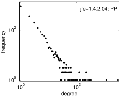
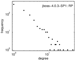
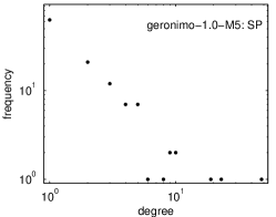
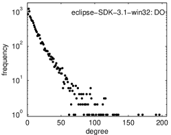
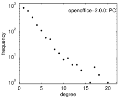
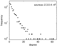
We consider the degree distributions of a variety of inter-class relationships in the Java source code of 12 different applications. These 12 programs are the largest of the 50 studied in Baxter et al. (2006). The actual programs (and version numbers) used are listed in Appendix B. Each metric counts for each type a certain kind of dependency on other types. We consider 14 metrics that can be identified as measuring either an out-degree or in-degree. Metrics used in Baxter et al. (2006) which could not be classified unambiguously as in- or out-degree distributions were left out. The metrics are defined in Appendix A, and each is referred to by a short abbreviation. Some pairs of metrics register opposite ends of the same relationship, suggesting that they are the out- and in- degree distributions of the same graph. However, considerations such as the separation of application code from shared libraries mean that the count of outgoing edges does not always match the total of incoming edges. We will not go into detail about the differences between the metrics, as our aim is simply to demonstrate the extent to which the model described below reproduces the patterns observed in these various data.

Plots of the 5 ‘in’ metrics (see Appendix A) on logarithmic axes often have a linear form, suggesting a power-law distribution is typical for graph in-degree distributions, regardless of the specific metric used or the particular program. Three examples are shown in Fig. 2, which shows the degree distributions for three different ‘in’ metrics (see Appendix A) in three different programs of differing sizes. The 9 ‘out’ metrics (see Appendix A) do not appear linear on doubly logarithmic axes, however a number of the plots do have a linear shape when plotted on linear-logarithmic axes, suggesting an exponential distribution.

Not all the data sets conform clearly to this pattern, having a slightly different shape or one or more points which do not fall on a neat curve. Nevertheless, the general pattern for in-degree is power-law like, and for out-degree seems to be an exponential shape. This suggests there is a common underlying process, modified to a greater or lesser degree by specific programmer actions in each case.

Software graph structures have been examined in several recent studies Myers (2003); Baxter et al. (2006); Wheeldon and Counsell (2003); Potanin et al. (2005); Valverde and Solé (2005a, b); Dong et al. (2006); Concas et al. (2007). In particular, several have reported power-law like degree distributions in graphs derived from source code Myers (2003); Wheeldon and Counsell (2003) or from object relationships at run-time Potanin et al. (2005). A distinction between in-degree and out-degree distributions has been observed in graphs derived from C and C++ software by Myers Myers (2003), who treated both as approximate power-law distributions, and Valverde and Solé Valverde and Solé (2005a),who in common with the present study of Java software, characterized the in-degree as a power-law and the out-degree as an exponential distribution. They showed that these distributions can be generated by certain cases of the GNC (‘growing network model with copying’) network growth model Krapivsky and Redner (2005), although the power law distribution generated by this model has a fixed exponent of 2. Yan, Qi and Gu Dong et al. (2006) examined Java applications, constructing the directed graph of ‘import’ relationships. Once again they note that the in-degree distribution typically resembles a power-law while the out-degree has a largely exponential behavior. Concas et al. Concas et al. (2007) also studied a Java application, and noted a difference between in-degree and out-degree distributions. These observations are confirmed by the present study of a much larger group of Java applications and metrics. Yan et al. also postulate a generative model for such distributions, but make no claims about its plausibility in relation to programmer actions.

Figure 3: Cumulative degree distribution of ‘out’ metrics (as labeled, see Appendix for definitions) for netbeans-4.1 with best fit model out-degree distribution (solid gray line) as described in Section II. Also shown for comparison is the best fit model in-degree distribution (dashed line). Horizontal scale is logarithmic and vertical scale is linear.

Figure 4: Cumulative degree distribution of ‘in’ metrics (as labeled, see Appendix for definitions) for the largest program studied, netbeans-4.1 with best fit model in-degree distribution (dashed gray line) as described in Section II. Also shown for comparison is the best fit model out-degree distribution (solid line). Horizontal scale is logarithmic and vertical scale is linear.

Figure 5: Top row: Degree distribution for AC (‘out’ metric) for three different programs (as labeled, see Appendix), on logarithmic-linear axes. Bottom row: Degree distribution for AP (the reciprocal ‘in’ metric) for the same three programs, on logarithmic-linear axes.

II Model

As programmers write software code, they will periodically add references between types (edges), and occasionally create new types (nodes). It is these aspects of the code we are interested in, so the intervening code, which is actually the majority of the program and specifies all its functions, is ignored. We consider a simplified process, each step of which entails either the addition of an edge between two existing nodes or the addition of a new node.

Generally there are a few elements that have many references to other parts of the program (these might be the most complex types), while there are many that reference only a few other types. This divergence can be approximated by ensuring that the “the rich get richer”, invoking the ‘cumulative advantage’ mechanism of Price de Solla Price (1976). New outgoing edges are added to the type which a programmer is ‘currently working on’, and we consider that the larger types (those with most out-edges already) are more likely to be added to in future. At each step a new edge is added, and the node the link originates from is chosen with a probability proportional to its current out-degree.

Conversely, there are a few elements that are referenced repeatedly by many of the other parts of the program (we might think of these as the simplest and most universal elements), while there are many that are used only a few times (these might be more complex elements, at a higher level of hierarchy, and therefore are less reusable). We consider the number of incoming dependencies a type has to be an approximation to it’s usefulness. Therefore the node to which a new edge will be linked is chosen with a probability proportional to its current in-degree.

The programmer is conscious of the number of outgoing references he or she is adding to a node, and at some point may decide the type is ‘too big’ and create a new one. This effect is represented by allowing new nodes to occasionally be created by ‘splitting’ an existing node into two pieces. The edges attached to the original node are divided between the two resulting nodes with each possible division between the two nodes of incoming and outgoing edges equally likely, with the constraint that at least one outgoing edge must be transferred to the new type, and one incoming edge must remain in the original type. Finally, if we think of the new node as carrying out a subset of the ‘task’ originally intended for the parent node, the two nodes must be connected, so a new edge is created from the original type to the new type. This also ensures that at all times every node has at least one incoming edge and one outgoing edge.

Let $v_{i}$ be the out-degree of node $i$, and $w_{i}$ be its in-degree, with $i$ running from $1$ up to $k$, the current number of nodes. All of these quantities can grow as the process proceeds. Let $t$ be the number of steps carried out so far. Since exactly $1$ edge is added at each step, $\sum_{i}v_{i}=\sum_{i}w_{i}=t$. The process is initiated at $t=1$ with a single node (type) with a single reference to itself (this is necessary, as links are only added to nodes which already possess links), i.e. $k=1$ and $v_{1}=w_{1}=1$. At each step:

• select parent node $m$ with probability $v_{m}/t$

• With probability $(1-\gamma)$ simply add an edge:

  • the parent node $m$ is the out node,

  • select in node $n$ with probability $w_{n}/t$,

  • $v_{m}\to v_{m}+1$ and $w_{n}\to w_{n}+1$.

• Otherwise, with probability $\gamma$, split the parent node:

  • add a new node $k+1$ (the last node number increments from $k\to k+1$),

  • choose $r$ uniformly from $\{1,...,v_{m}\}$ and $s$ uniformly from $\{0,...,w_{m}-1\}$, then
    $v_{k+1}\to r$, $v_{m}\to v_{m}-r+1$;
    $w_{k+1}\to s+1$ and $w_{m}\to w_{m}-s$.

• Increment the counter $t\to t+1$.

These steps are repeated for some predetermined number of steps $t_{final}$. The entire simulation is defined by only two parameters: the total number of links required (equal to the number of simulation steps), $t_{final}$, and the splitting probability, $\gamma$. Since new types only appear due to the splitting process, $\gamma$ determines the ratio between the number of types and the number of links: $\frac{k}{t}\to\gamma\mbox{ as }t\to\infty$. Note that although nodes to be ‘worked on’ are selected according to their out-degree, this model is actually symmetric with respect to in- and out-degree, except for the splitting step: nodes acquire outgoing edges at a rate proportional to their existing out-degree, and acquire incoming edges at a rate proportional to their in-degree. In this model edges are added one by one to different parts of the graph, so all the types grow at the same time. New nodes are also created during this process. This doesn’t necessarily reflect the actual order in which program code is written.

Although the graph continues to grow, after a sufficient number of steps, the relative degree frequencies – normalized by the total number of nodes – reach an equilibrium distribution. Let $C_{m}$ be the number of types with out-degree $m$ after step $t$. Considering the two processes involved in the model, $C_{m}$ can increase by 1 if an outgoing edge is added to a type with out-degree $m-1$ and is not split, or if a type with out-degree greater than $m$ is split at just the right place that one of the resulting types has out-degree $m$. Similarly, $C_{m}$ decreases if a type of size $m$ gains a new out-link, or is split, so long as the point of splitting is not $1$ or $m$. With a little consideration, we can write down the expected change in $C_{m}$ at the next step:

$$\langle\delta C_{m}\rangle=(1-\gamma)(m-1)C_{m-1}+\gamma\sum_{r>m}rC_{r}\frac{2}{r}$$

$$-(1-\gamma)mC_{m}-\gamma mC_{m}(1-\frac{2}{m})\;.$$ (1)

The expected fraction of types that have degree $m$ is

$$f_{m}=\frac{\langle{C_{m}(t)}\rangle}{\langle k(t)\rangle}\;.$$ (2)

It follows from the definition that $\langle\delta C_{m}\rangle=\gamma f_{m}$. Substituting back into (II) we find after collecting like terms that

$$(1+m-2\gamma)f_{m}=(1-\gamma)(m-1)f_{m-1}+2\gamma\sum_{r=m+1}^{R}f_{r}\;.$$ (3)

This equation is valid for all $m>1$. Replacing $m$ by $m-1$ in (3), rearranging for the summation term and substituting back into the original version of (3) gives $f_{m}$ in terms of $f_{m-1}$ and $f_{m-2}$ , and after calculating $f_{1}$ and $f_{2}$ explicitly we find by induction the solution for general $m$ to be

$$f_{m}=\gamma(1-\gamma)^{m-1}\;,$$ (4)

which can be written as an exponential $f_{m}=\frac{\gamma}{1-\gamma}e^{-\beta m}$ where $\beta=-\ln(1-\gamma)$.

A similar calculation can be performed for the in-degree distribution. The in-degree and out-degree of a type are completely independent, so the selection of a type for splitting is uniform with respect to in-degree. If $g_{n}$, in analogy to $f_{m}$, is the fraction of types with in-degree $n$ we find that

$$g_{n}\left[2\frac{n-1}{n}+(1-\gamma)n\right]=2\sum_{l>n}\frac{g_{l}}{l}+(1-\gamma)(n-1)g_{n-1}\;.$$ (5)

Using a similar method to before we find

$$g_{n}=\frac{(1-\gamma)n}{2+(1-\gamma)n}g_{n-1}\;,$$ (6)

so that

$$g_{n}=\frac{\Gamma(n+1)\Gamma(2+\frac{2}{1-\gamma})}{\Gamma(n+1+\frac{2}{1-\gamma})}g_{1}\;,$$ (7)

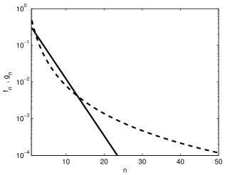
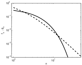
and normalization can be used to find $g_{1}$. For large $n$, the ratio $g_{n}/g_{n-1}$ tends to $1-\frac{2}{(1-\gamma)n}$, that is, the in-degree distribution tends to a power-law of the form $g_{n}=cn^{-\alpha}$ with exponent $\alpha=2/(1-\gamma)$. Thus the model predicts a decaying exponential for the out-degree distribution, and an in-degree distribution with a power-law tail with exponent greater than or equal to $2$. Examples of the two distributions (4) and (7) are shown in Fig. 6.

Figure 6: Examples of the degree distributions generated by the model, with parameter $\gamma=0.3$. Solid line is the out-degree model,$f_{n}$, dashed line the in-degree model, $g_{n}$. On linear-logarithmic axes, top, and double logarithmic axes, bottom.

III Comparison with measured data

The distributions (4) and (7) were fitted to the data described in Section I using a maximum likelihood method, which is asymptotically unbiased Barnsdorff and Cox (1994) . Given some candidate distribution $f(x,\gamma)$, the likelihood that the histogrammed data $h_{i}$ at values $x_{i}$ was generated from this distribution, given the parameter $\gamma$, is

$$p(\mathbf{h}|\gamma)=\prod_{i=1}^{k}f(x_{i},\gamma)^{h_{i}}$$ (8)

and we proceed by finding the value of $\gamma$ which maximizes this quantity. In the case of out metrics, $f(x_{i},\gamma)$ is given by (4), and the maximum likelihood estimator (MLE) of $\gamma$ is found analytically to be

$$\hat{\gamma}=\frac{k}{t}$$ (9)

as expected, where $t=\sum_{i}x_{i}h_{i}$ is the number of edges in the graph, and $k=\sum_{i}h_{i}$ is the number of nodes. For in metrics, we use (7), for which we have not been able to find a similar solution so the MLE of $\gamma$ must be found numerically. We again expect $\gamma=k/t$ because this was assumed in the derivation of (7), although in some cases this is not the best fit value. The explanation of this is not known, though this very simple model is not expected to explain every detail of the data.

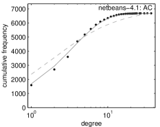
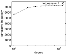
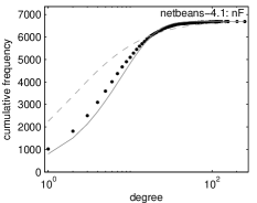
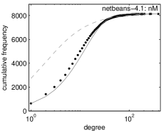
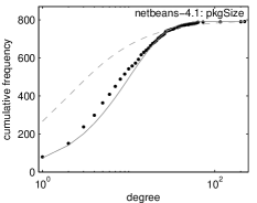
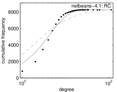
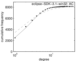
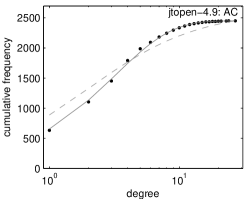
The cumulative distribution derived from function (4) using the best fit (MLE estimated) $\gamma$ value is plotted along with the out metric data in Fig. 4. This figure plots all of the out-metrics for the same program, netbeans-4.1, and it can be seen that in the majority of cases the agreement with the data is reasonably good, even though the number of nodes in the graphs for different metrics varies widely. Further examples are shown in the top half of Fig. 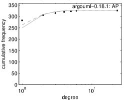5, which shows the same metric, AC, for three different programs. Notice also that a fit of the ‘wrong’ model distribution (the predicted in-degree distribution) does not fit as well. 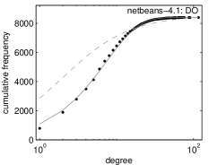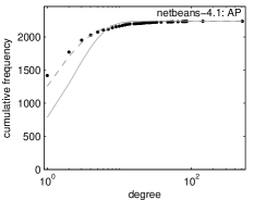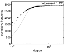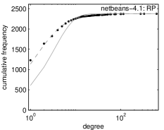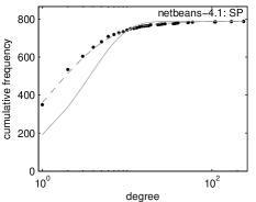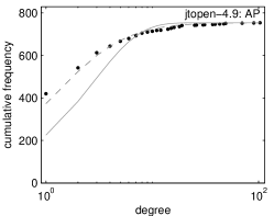Similarly, the cumulative best-fit functions (7) for each of the in metrics for netbeans-4.1 is plotted in Fig. 4, and for three different programs for the same metric (AP) in the bottom half of Fig. 5. Again, many data sets show good agreement, and the in-degree model fits the data much better than the out-degree model (solid curve). Comparisons were made for all the metrics and programs listed in Appendices A and B and Figs. 4, 4 and 5 are fairly representative. 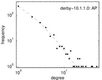An example of one of the better fits to an out metric data set is shown in Fig. 8, and an example of a good in metric fit in Fig. 8.

Figure 7: AC for columba-1.0, an example of an out metric distribution that is well fitted by the model.

Figure 8: AP for derby-10.1.1.0, an example of an in metric distribution that is well fitted by the model.

To obtain a quantitative measure of how well the model fits the data, we follow the method of Clauset et al. (2007) and calculate a $p$-value (the probability that the data were drawn from the proposed distribution) based on the Kolmogorov-Smirnov (KS) statistic Kendall and Stuart (1979)

$$D=\mbox{max}|S(x)-F(x)|$$ (10)

where $S(x)$ is the cumulative distribution function (CDF) of the data and $F(x)$ is the CDF of the proposed distribution (i.e. $F(x)=\sum_{y\leq x}f(x)$). The fitted distribution is correlated with the data, so treating it as the true distribution will give a falsely high $p$-value. Instead we use a Monte Carlo procedure, following Clauset et al. (2007): A large number of synthetic data sets is drawn from the best-fit distribution, each one is fitted individually and the KS statistic (relative to its own best fit distribution) calculated for each of these fits. The $p$-value is then the fraction of these KS statistic values that are larger than that found for the original fit to the real data.

Table 1: Number of $p$-values greater than 0.05 and 0.1 for the out-degree and in-degree data sets.

	# $p$-values		# $p$-values
	$>0.05$	%	$>0.1$	%
out-metrics	4 / 101	4%	4 / 101	4%
in-metrics	9 / 44	20%	8 / 44	18%

The $p$-values calculated for the in metrics and out metrics are tabulated in Table 1. We see that quantitatively, the fits are not particularly good. The goodness of fit for out metrics is particularly poor. The in metrics are often reasonably well fit by the model, but where the fit fails, it is sometimes because the degree one point is lower than predicted – see for example Doinv for netbeans-4.1 in Fig. 4. In other cases, the distribution appears to be a more pure power law than the model function. Overall, the heavy tail of the in degree distribution predicted by the model is successfully observed. The model fits to out metric distributions are generally worse than those for the in metrics and often have a more complicated shape, supporting the hypothesis that the difference between the distributions is the direct programmer intervention in the out-degrees of types. The KS statistic is the maximum difference between the model and data cumulative distributions, and we see from Fig. 4 that although the shapes are similar, there is separation between the two curves over part of the range in several cases, destroying the quantitative goodness of fit. Nevertheless, the model appears to fit many of the curves well or be qualitatively in agreement for much of the range.

Two assumptions of the model are that types gain edges at a rate proportional to the existing number of edges, and that when a type is subdivided the redistribution of edges between the two resulting types is uniform. If the selection of nodes to which new edges are attached is uniform rather than linear, the resulting in-degree distribution has an exponential tail, which is not the case in real software graphs, so it appears that it is necessary that the rate of attachment of new edges to a node should depend on the existing degree of the node, though the explanation for this is not as clear as in the case of wealth distribution or paper citation rates.

In the current model, new types are created by removing references (edges) from an existing type and placing it in a new type. It is equally plausible that a programmer instead copies references, creating duplicates of edges. If this is the case, and none of the edges are transferred to the new node the out-degree distribution has a ‘fatter’ tail than the original exponential distribution, but the ‘head’ of the distribution also becomes much steeper, meaning that this model fits the out-degree distribution data very poorly. Alternatively if the edges are distributed between the two nodes according to a binomial distribution (so that each edge is equally likely to be attached to either node), the resulting out-degree distribution has a distribution similar to an exponential distribution, and the in-degree distribution has a power-law tail with a minimum exponent of $3$. This is also incompatible with the data, which typically have a power-law tail with exponent close to $2$.

IV Discussion

In this paper we have described a simple model of the generation of software graph degree distributions based on the assumption that the process of programming involves programmers making active choices about the structure of the type on which they are working – in particular they are conscious of the ‘size’ of the type, and this comes to be reflected in the resulting out-degree, while the in-degree of a type emerges indirectly as a result of the construction of other types. The only difference between incoming and outgoing edges in the microscopic process of the model is that the splitting operation on types is dependent on type out-degrees and is independent of in-degrees. This model is extremely simple, and depends on a single parameter $\gamma$ which can be physically interpreted as the reciprocal of the average degree of the graph. This suggests that the mean number of dependencies per type (both incoming and outgoing) may prove to be a useful statistic for comparing different type relationships and different programs. The model reproduces the approximate shapes of in-degree and out-degree distributions for a range of graph construction metrics applied to a variety of Java programs. This suggests that this shape is due to simple statistical processes common to all software graphs, so that any differences due to different design methodologies and so on must be sought in the details of the deviations from this mean behavior. The agreement of the proposed model with the measured data is not perfect however. These and other difficulties, such as variations between the shapes of distributions between programs and between metrics indicates that there are higher-order effects that remain to be described.

Degree distribution is one of the most accessible measures of the ‘shape’ of a network, but there are many more measures such as degree correlation, clustering coefficients and so on that can be calculated. Further analysis of real data sets for such more detailed measures would help to discriminate between and to refine the various generative models that have so far been proposed. Another avenue of investigation that would be particularly fruitful would be a statistical analysis of the programming process as it happens, in order to identify the rates and probabilities of various actions, which could then be compared with the assumptions of the model proposed in this paper.

Appendix A metrics

Brief descriptions of the metrics used in the study are listed below. Following Wheeldon and Counsell (2003); Baxter et al. (2006) short codes are used throughout the text to refer to each metric. For more complete descriptions of the metrics and how the data was extracted from the source code, see Baxter et al. (2006).

Some of the metrics are paired, with one representing the ‘in’ degree (listed first) and another representing the reciprocal ‘out’ degree. In general an ‘out’ metric for a type counts things that would appear in the code for that type, while ‘in’ metrics count references to a type which appear in the code for other types. Some of the metrics have no reciprocal metric, but can still be identified as measuring either ‘in’ or ‘out’ degree. The remaining metrics used in Baxter et al. (2006) were not included in the analysis as their in/out status was not clear or they were a mixture of in and out measures.

‘In’ metrics

AP References to class as a member.

For a given type, the number of top-level types (including itself) in the source that have a field of that type.

DOinv Depends On inverse.

For a given type, the number of type implementations in which it appears in their source.

PP References to class as a parameter.

For a given type, the number of top-level types in the source that declare a method with a parameter of that type.

RP References to class as return type.

For a given type, the number of top-level classes in the source that declare a method with that type as the return type.

SP Subclasses.

For a given class, the number of top-level classes that specify that class in their extends clause.

‘Out’ metrics

AC Members of class type.

For a given type, the size of the set of types of fields for that type.

DO Depends on.

For a given type, the number of top-level types in the source that it needs in order to compile.

PC Parameter-type class references.

For a given type, the size of the set of types used as parameters in methods for that type.

PubMC Public Method Count.

The number of methods in a type with public access type.

RC Methods returning classes.

For a given type, the size of the set of types used as return types for methods in that type.

nC Number of Constructors.

For a given class, the number of constructors of all access types declared in the class.

nF Number of Fields.

For a given type, the number of fields of all access types declared in the type.

nM Number of Methods.

For a given type, the number of all methods of all access types (that is, public, protected, private, package private) declared (that is, not inherited) in the type.

pkgSize Package Size.

The number of types contained direction in a package (and not contained in sub-packages).

Appendix B applications

The programs studied, their size (number of Classes), domain and where they were sourced are:

Application	#Classes	Domain	Origin	Notes
eclipse-SDK-3.1-win32	11413	IDE	www.eclipse.org	Donated by IBM
netbeans-4.1	8406	IDE	netbeans.org	Donated By Sun
jre-1.4.2.04	7257	JRE	sun.com
jboss-4.0.3-SP1	4143	J2EE server	Sourceforge
openoffice-2.0.0	2925	Office suite	openoffice.org	Donated By Sun
jtopen-4.9	2857	Java toolbox for iSeries and AS/400 servers	Sourceforge	Donated by IBM
geronimo-1.0-M5	1719	J2EE server	Apache
azureus-2.3.0.4	1650	P2P filesharing	Sourceforge
derby-10.1.1.0	1386	SQL database	Apache Jakarta	Donated by IBM
compiere-251e	1372	ERP and CRM	Sourceforge
argouml-0.18.1	1251	UML drawing/critic	tigris.org
columba-1.0	1180	Email client	Sourceforge

References

- Baxter et al. (2006) G. Baxter, M. Frean, J. Noble, M. Rickerby, H. Smith, M. Visser, H. Melton, and E. Tempero, in Proceedings of the 21st Annual ACM SIGPLAN Conference on Object-Oriented Programming, Systems, Languages, and Applications, edited by R. Johnson and R. P. Gabriel (ACM, 2006), in press.
- Dong et al. (2006) Y. Dong, Q. Guo-Ning, and G. Xin-Jian, Chinese Physics 15, 2489 (2006).
- Myers (2003) C. R. Myers, Physical Review E 68, 046116 (2003).
- Potanin et al. (2005) A. Potanin, J. Noble, M. Frean, and R. Biddle, Communications of the ACM 48, 99 (2005).
- Valverde and Solé (2005a) S. Valverde and R. V. Solé, Europhysics Letters 72, 858 (2005a).
- de Solla Price (1976) D. de Solla Price, Journal of the American Society for Information Science 27, 292 (1976).
- Wheeldon and Counsell (2003) R. Wheeldon and S. Counsell, in Third IEEE International Workshop on Source Code Analysis and Manipulation (SCAM03) (2003).
- Valverde and Solé (2005b) S. Valverde and R. V. Solé, Physical Review E 72, 026107 (2005b).
- Concas et al. (2007) G. Concas, M. Marchesi, S. Pinna, and N. Serra, IEEE Transactions on Software Engineering 33, 687 (2007).
- Krapivsky and Redner (2005) P. L. Krapivsky and S. Redner, Physical Review E 71, 036118 (2005).
- Barnsdorff and Cox (1994) O. E. Barnsdorff and D. R. Cox, Inference and Asymptotics, Monographs on Statistics and Applied Probability (Chapman and Hall, London, 1994).
- Clauset et al. (2007) A. Clauset, C. R. Shalizi, and M. E. J. Newman, Preprint, arXiv:0706.1062 (2007).
- Kendall and Stuart (1979) M. Kendall and A. Stuart, The Advanced Theory of Statistics, vol. 2 (Charles Griffin, 1979), 4th ed.