Production of Magnetic Turbulence by Cosmic Rays Drifting Upstream of Supernova Remnant Shocks

Abstract

We present results of two- and three-dimensional Particle-In-Cell simulations of magnetic-turbulence production by isotropic cosmic-ray ions drifting upstream of supernova remnant shocks. The studies aim at testing recent predictions of a strong amplification of short-wavelength magnetic field and at studying the subsequent evolution of the magnetic turbulence and its backreaction on cosmic ray trajectories. We observe that an oblique filamentary mode grows more rapidly than the non-resonant parallel modes found in analytical theory, and the growth rate of the field perturbations is much slower than is estimated for the parallel plane-wave mode, possibly because in our simulations we cannot maintain $\omega\ll\Omega_{i}$, the ion gyrofrequency, to the degree required for the plane-wave mode to emerge. The evolved oblique filamentary mode was also observed in MHD simulations to dominate in the non-linear phase, when the structures are already isotropic. We thus confirm the generation of the turbulent magnetic field due to the drift of cosmic-ray ions in the upstream plasma, but as our main result find that the amplitude of the turbulence saturates at about $\delta B/B\sim 1$. The backreaction of the magnetic turbulence on the particles leads to an alignment of the bulk-flow velocities of the cosmic rays and the background medium. This is an essential characteristic of cosmic-ray modified shocks: the upstream flow speed is continuously changed by the cosmic rays. The deceleration of the cosmic-ray drift and the simultaneous bulk acceleration of the background plasma account for the saturation of the instability at moderate amplitudes of the magnetic field. Previously published MHD simulations have assumed a constant cosmic-ray current and no energy or momentum flux in the cosmic rays, which excludes a backreaction of the generated magnetic field on cosmic rays, and thus the saturation of the field amplitude is artificially suppressed. This may explain the continued growth of the magnetic field in the MHD simulations. A strong magnetic-field amplification to amplitudes $\delta B\gg B_{0}$ has not been demonstrated yet.

1 INTRODUCTION

The prime candidate for the sources of Galactic cosmic rays are shell-type supernova remnants (SNRs), at whose forward shocks a Fermi-type acceleration process could accelerate particles to PeV-scale energy, although no firm evidence has been established to date for hadron production in SNRs. The acceleration arises from pitch-angle scattering in the plasma flows that have systematically different velocities upstream and downstream of the shock (Bell, 1978). More detailed studies show that the acceleration efficacy and the resulting spectra depend on the orientation angle of the large-scale magnetic field and on the amplitude and characteristics of magnetic turbulence near the shock (e.g. Giacalone & Jokipii, 1996; Giacalone, 2005; Pelletier et al., 2006; Marcowith et al., 2006). Particle confinement near the shock is supported by self-generated magnetic turbulence (Malkov & Diamond, 2001), which is likely generated in the upstream region. As the flow convects the turbulence toward and through the shock, the turbulent magnetic field structure at and behind the shock is shaped by the plasma interactions ahead of it. Therefore, detailed knowledge of the properties of the turbulence is crucial to ascertain all aspects of the acceleration processes: transport properties of cosmic rays, the shock structure, thermal particle injection and heating processes. Of particular interest is the question of how efficiently and with what properties electromagnetic turbulence is produced by energetic particles at some distance upstream of the forward shocks. If the cosmic rays would drive a turbulent magnetic field to an amplitude much larger than the homogeneous interstellar field (Lucek & Bell, 2000; Bell & Lucek, 2001), particle acceleration could be faster and extend to higher energies than conventionally estimated (Lagage & Cesarsky, 1983), although it is unclear what energies could be reached (Vladimirov et al., 2006; Ellison & Vladimirov, 2008).

We investigate the properties of magnetic turbulence upstream of the shocks of young SNRs. Cosmic rays accelerated at these shocks form a nearly isotropic population of relativistic particles that drift with the shock velocity relative to the upstream plasma. Even though the shock may accelerate particles over a wide range of energies, the highest-energy particles propagate the farthest from the shock, so at some distance upstream one finds only particles of the highest energy, which are predominantly ions. Such a system has been recently studied by Bell (2004, hereafter denoted as B04) with a quasi-linear MHD (Magnetohydrodynamics) approach. Bell noted that, rather than resonant Alfvén waves, the current carried by drifting cosmic rays should efficiently excite non-resonant, nearly purely growing ($\Re\,\omega=\omega_{\rm R}\simeq 0$) modes of magnetic turbulence. The analytical results were reproduced in studies by Bykov & Toptygin (2005) and Pelletier et al. (2006), who noted the need to carefully account for the return current, and Zirakashvili et al. (2008, hereafter denoted as Z08). Calculations by Blasi & Amato (2007) and Reville et al. (2007) using the linearized Vlasov equation confirmed the predictions of the MHD approximation. Bell (2005, hereafter denoted as B05) noted that a filamentation of the background plasma must be expected as soon as a small current imbalance occurs, which may eventually give rise to a filamentation of the cosmic-ray current. MHD simulations described by B04, B05 and Z08 indicate a strong magnetic-field amplification following a plasma filamentation that turns approximately isotropic in the non-linear stage. The results presented in those papers do not indicate that a parallel plane-wave mode is initially observed.

Here we use Particle-In-Cell (PIC) simulations with a view to explore the properties of the magnetic turbulence produced: its geometry, non-linear evolution, saturation, and associated particle heating. Our kinetic approach also allows us to address the backreaction of the magnetic turbulence on cosmic rays.

We describe the simulation setup in §2, where we also present a rationale for selecting sets of simulations according to the theoretical analyses. In §3 the simulation results are presented starting with the main three-dimensional experiment, including a discussion of scaling and parameter dependences, and the evolution of the particle spectra. We conclude with a summary and discussion in §4.

2 SIMULATION SETUP

2.1 Simulation Method and Initial Conditions

Our discussion of the production of magnetic turbulence by the non-resonant streaming instability is based on three-dimensional PIC experiments. However, performing large-scale simulations in three dimensions poses serious computational demands. Simulations of two-dimensional systems can address problems that involve a wider range of spatial scales, or growth on timescales long compared with the electron plasma periods, and therefore our three-dimensional experiments are complemented by a series of two-dimensional simulations. The two-dimensional runs allow us to study the evolution of magnetic turbulence at timescales for which the turbulent field structures become larger than the extent of the three-dimensional simulation box, and so they enable us to ascertain the influence of the limited size of the simulation box on the results of the 3-D experiments. Furthermore, the two-dimensional runs permit us to study how these results depend on the choice of physical parameters of the simulations.

The code used in this study is a modified parallel version of TRISTAN (Buneman, 1993), a three-dimensional fully relativistic electromagnetic Particle-In-Cell code in Cartesian coordinates. The modifications to the code include the use of a new first-order algorithm for the charge-conserving current deposition developed by Umeda et al. (2003), and the implementation of a new method of digital filtering of electric currents. The filtering method uses the set of 27-point-average isotropic smoothing and compensation filters, which attenuate the short-wavelength noise, increase the overall accuracy, and at the same time improve agreement with theory at long wavelengths (see, e.g., Birdsall & Langdon, 2005). The two-dimensional simulations have been performed using the same three-dimensional code, in which the grid size in one dimension was restricted to contain three cells only. We thus follow the temporal evolution of all three vector components of particle velocities and the electromagnetic fields, and can therefore accurately simulate circularly polarized waves as found in the analytical theory, requiring only that the wavevector lies in the simulation plane. However, a filamentation mode may appear somewhat different in two dimensions.

In the simulations, an isotropic population of relativistic, monoenergetic cosmic-ray ions with Lorentz factor $\gamma_{CR}=2$ and number density $N_{CR}$ drifts with $v_{sh}=0.3c$ relative to the upstream electron-ion plasma and along a homogeneous magnetic field $B_{\parallel 0}$, carrying a current density $j_{CR}=eN_{CR}v_{sh}$. The ions of the upstream medium have a thermal distribution with number density $N_{i}$, in thermal equilibrium with the electrons. The electron population with thermal velocity $v_{e,th}=0.002c$ and density $N_{e}=N_{i}+N_{CR}$ contains the excess electrons required to provide charge-neutrality and also drifts with $v_{d}=v_{sh}N_{CR}/N_{e}$ with respect to the upstream ions, so it provides a return current $j_{ret}=-eN_{e}v_{d}$ to balance the current in cosmic rays. We assume that the return current is entirely carried by the electron component of the background plasma because that will most quickly react to an electric field induced by charge separation due to the drifting cosmic-ray component. The simulations have been performed using computational grids with periodic boundary conditions (see Table 1), which keeps the particle number constant throughout the simulations at a value corresponding to an average total density of 16 particles per cell. A two-dimensional test simulation with 160 particles per cell has also been run to verify that the number of particles used in our studies does not significantly influence the results.

Cosmic-ray ions drift in the $-x$-direction, antiparallel to the homogeneous magnetic field $B_{\parallel 0}$. For the two-dimensional simulations we render the $z$-coordinate ignorable, so the direction of the drift is in the simulation plane. The electron skindepth $\lambda_{se}=c/\omega_{pe}=7\Delta$, where $\omega_{pe}=(N_{e}e^{2}/m_{e}\epsilon_{0})^{1/2}$ is the electron plasma frequency and $\Delta$ is the grid cell size. The parameter combination is chosen both to resemble physical conditions in young SNRs and, according to the quasi-linear calculations by B04, to be favorable for the rapid excitation of purely growing, short-wavelength (as compared with cosmic-ray ion gyroradii $r_{CRg}$) wave modes, although we typically cannot maintain the condition $\omega\ll\Omega_{i}$. For a cold ambient plasma and for wavevectors $k_{\parallel}$ parallel to $B_{\parallel 0}$, the dispersion relation in the unstable wavevector regime $1<k_{\parallel}r_{CRg}<\zeta v_{sh}^{2}/v_{A}^{2}$ reads

$$\omega^{2}-v_{A}^{2}k^{2}_{\parallel}+\zeta v_{sh}^{2}\,\frac{k_{\parallel}}{r_{CRg}}=0,$$ (1)

for which purely growing solutions are found. The maximum growth rate $\gamma_{max}$ at the wavenumber $k_{\parallel max}$ can be determined as

$$k_{\parallel max}=\frac{\zeta}{2}\frac{v_{sh}^{2}}{v_{A}^{2}}\frac{1}{r_{CRg}}\;\;\;\;\;{\rm and}\;\;\;\;\;\gamma_{max}=\frac{\zeta}{2}\frac{v_{sh}^{2}}{v_{A}}\frac{1}{r_{CRg}}.$$ (2)

Here, $r_{CRg}=m_{i}c\sqrt{\gamma_{CR}^{2}-1}/eB_{\parallel 0}$ is the gyroradius of the (lowest-energy) cosmic rays, $v_{A}=[B_{\parallel 0}^{2}/\mu_{0}(N_{e}m_{e}+N_{i}m_{i})]^{1/2}$ is the Alfvén velocity, and $\zeta=N_{CR}c\sqrt{\gamma_{CR}^{2}-1}/N_{i}v_{sh}$ determines the strength of the cosmic-ray driving term. From Eq. (1) one can see that the non-resonant modes are strongly driven when $\zeta v_{sh}^{2}/v_{A}^{2}\gg 1$. For the given parameters, this condition depends on the magnetic field strength and the ion-electron mass ratio, which also determine the wavelength $\lambda_{max}=2\pi/k_{max}$ of the most unstable mode. This wavelength must be much smaller than the size of the computational box to enable studies of the evolution of the turbulence towards larger scales, and at the same time it must be clearly separated from the physical scales in the background plasma. Restricted by these computational requirements, for the main three-dimensional experiment (run A) we assume a density ratio $N_{CR}/N_{i}$=1/3 and a reduced ion-electron mass ratio $m_{i}/m_{e}=10$, which gives the ion skindepth $\lambda_{si}=25.3\Delta$ and sets the wavelength of the most unstable mode to $\lambda_{max}=50\Delta$. With this choice we have further specified $\zeta v_{sh}^{2}/v_{A}^{2}\simeq 715$, the Alfvénic Mach number $M_{A}=v_{sh}/v_{A}=19.1$, and the ratio $\omega_{pe}/\Omega_{e}=22.1$, where the electron cyclotron frequency $\Omega_{e}=eB/m_{e}$, which corresponds to weakly magnetized conditions of the interstellar medium. The periodic boundary conditions allow us to follow the gyration motion of cosmic rays, even though the cosmic-ray ion gyroradii, $r_{CRg}\simeq 2672\Delta$, are much larger than the size of the simulation box, which is 19.8$\times$6.1$\times$6.1 in units of $\lambda_{max}$.

2.2 Simulation Parameters

Table 1 compares the parameters and main results of all runs in two and three dimensions with those of the initial three-dimensional experiment. The follow-up simulations were mainly used to probe systems with more realistic mass ratios up to $m_{i}/m_{e}=500$, better separated spatial scales $\lambda_{si}$ and $\lambda_{max}$, smaller density ratios $N_{CR}/N_{i}$, and also to allow the box size to be a higher multiple of the wavelength of the most unstable mode. Run A^∗ uses the parameters of run A in a large two-dimensional box of size 50$\times$18 $\lambda_{max}$ and is performed to confirm that the results of two-dimensional runs are similar to those of the three-dimensional simulations. Runs B to E use larger ion-electron mass ratios, whereas runs G to J are for smaller density ratios.

Note that in runs B to E the ion skindepth $\lambda_{si}$ increases with mass ratio as $(m_{i}/m_{e})^{1/2}$, and thus $\lambda_{max}$ needs to be readjusted to separate the plasma and turbulence scales. The wavelength of the most unstable mode is thus increased by increasing the strength of the homogeneous magnetic field $B_{\parallel 0}$ by approximately the same factor $(m_{i}/m_{e})^{1/2}$. In this way the ratio $\lambda_{max}/\lambda_{si}$ and the Alfvén Mach number $v_{sh}/v_{A}$ of the cosmic-ray drift of runs A and A^∗ are preserved in those runs, and also the dynamic range in wavelength, as given by $\zeta v_{sh}^{2}/v_{A}^{2}$, remains unchanged. However, the maximum growth rate $\gamma_{max}$ scales inversely with $(m_{i}/m_{e})^{1/2}$, and therefore the three-dimensional studies would clearly require an enormous computational effort, if more realistic mass ratios were assumed. We restrict the duration of these simulations (runs B and C) to cover only the initial stage of the instabilities, and the full non-linear evolution is investigated by means of two-dimensional simulations (runs D and E). Note that when the ion-electron mass ratio increases, the upstream plasma becomes more magnetized (the frequency ratio $\omega_{pe}/\Omega_{e}$ decreases; see Table 1), and the cosmic-ray gyroradii grow. For run E, in which $m_{i}/m_{e}=500$, these parameters are $\omega_{pe}/\Omega_{e}=3.3$ and $r_{CRg}\simeq 19722\Delta$. Finally, in run F the wavelength of the most unstable mode has been increased to $\lambda_{max}=150\Delta$ to allow for a better separation from the plasma scales. This is done by increasing the strength of the regular magnetic field $B_{\parallel 0}$, whereas the ion-electron mass ratio is kept the same as in run A. This means that in this case the Alfvén Mach number decreases to $M_{A}=6.3$ and also the width of the unstable wavevector range, here $\zeta v_{sh}^{2}/v_{A}^{2}\simeq 80$, is an order of magnitude smaller compared with the other runs. For the parameters of run F, the ratio $\omega_{pe}/\Omega_{e}=7.4$ and $r_{CRg}\simeq 890\Delta$.

The runs G to J have been performed for smaller values of the density ratio $N_{CR}/N_{i}$ down to 1/30, which implies a smaller drift velocity of the electrons in the background plasma. This reduces the impact of an initial electrostatic, Buneman-type instability, so less heating will occur initially and the plasma temperature should be lower throughout the simulation. The mass ratio is $m_{i}/m_{e}=50$ in these simulations ($\lambda_{si}=51.9\Delta$), which cover a range in plasma magnetizations with parameters ranging from $M_{A}=13$ and $\lambda_{max}=500\Delta$ to $M_{A}=65$ and $\lambda_{max}=100\Delta$. In all simulations the time step $\delta t=0.0715/\omega_{pe}$.

3 RESULTS

3.1 Three-dimensional Experiment

The temporal evolution of the magnetic and electric fields and the particle kinetic-energy densities in the three-dimensional simulation (run A) is shown in Fig. 1. An initial (up to $t\sim\gamma_{max}^{-1}$) fast growth of the turbulent fields is caused by a Buneman-type beam instability between drifting electrons and the ambient ions, which leads to plasma heating until the electron thermal velocities become comparable to the electron drift speed $v_{d}$ (recall that the electrons in the background plasma must slowly drift to initially compensate the cosmic-ray current). found in the analytical theory In real SNRs the density ratio $N_{e}/N_{CR}$ is likely much larger than the sonic Mach number, and therefore the electron drift speed is smaller than their thermal velocity. The initial instability is thus solely a consequence of the initial conditions in our simulations, in particular the initial temperature of the background medium and the density contrast between cosmic rays and the background plasma.

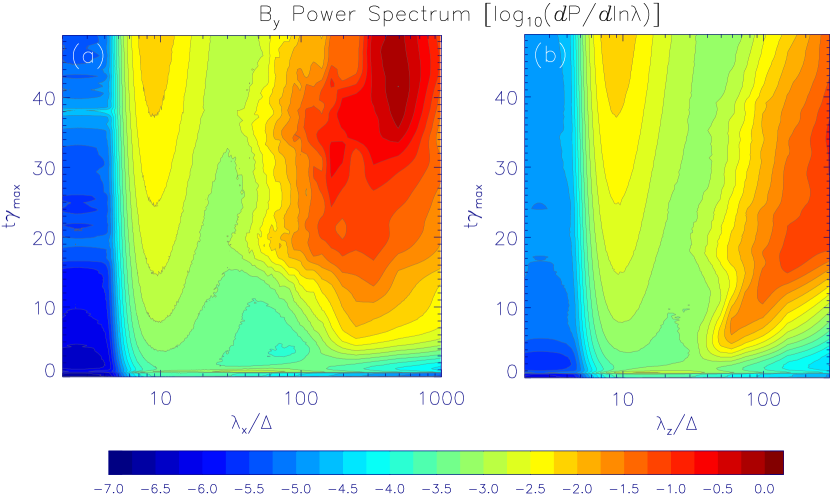
Figure 2: The time evolution of the Fourier power spectrum of the perpendicular magnetic-field component $B_{y}$ in run A. The spectra in wavelengths along the drift direction $\lambda_{x}=2\pi/k_{\parallel}$ are shown in the left panel (a), whereas spectra for the direction perpendicular to both the drift velocity and $B_{y}$ are displayed in the right panel (b). Note that at small wavelengths ($\lambda\leq 5\Delta$) strong filtering reduces the Fourier power to very small values. The spectra are normalized to the peak spectral density.

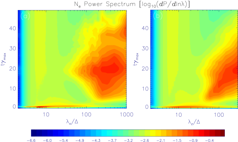
Figure 3: The temporal evolution of the electron-density power spectrum for run A. The spectra are set up as described in Fig. 2 and normalized to the peak spectral density.

At $t\sim 2.5\,\gamma_{max}^{-1}$ wave modes start to emerge that are excited by the cosmic-ray ions streaming in the upstream plasma, and turbulent magnetic field is seen mainly in the components transverse to the cosmic-ray drift direction. A plane-wave Fourier analysis is shown in Fig. 2 for one component of the magnetic field and in Fig. 3 for the density of the background electrons. All Fourier power spectra are averages over the simulation box to reduce the noise. Note that for a plane wave of wavelength $\lambda$ propagating at an angle $\theta$ to the drift ($-x$) direction, the one-dimensional Fourier spectra will reveal a signal at $\lambda_{\parallel}=\lambda_{x}=\lambda/\cos\theta$ and at $\lambda_{\perp}=\lambda_{z}=\lambda/\sin\theta$, respectively. Assuming a plane wave as in the analytical calculations of B04 we therefore conclude that the dominant wave mode is oblique at an angle of about $\theta\approx 80^{\circ}$ to the $x$-direction, and has the perpendicular wavelength component $\lambda_{\perp}\simeq 50\Delta$, which is numerically similar to $\lambda_{max}$. The character of the mode is thus different than predicted by the quasi-linear analysis (B04, B05), which indicated that initially the most rapid growth should occur for wavenumbers parallel to $B_{\parallel 0}$ (see also Eq. 1). Here we observe a modified filamentation instability, which appears to be faster than the non-resonant parallel modes and was also observed in MHD simulations (B04, B05, Z08 Reville et al. (2008a)) to dominate in the non-linear phase. At that time, when $\delta B>B_{\parallel 0}$ is already established, the field structures in the MHD studies have the same spatial scales parallel and perpendicular to the cosmic-ray drift direction, as evident from Figure 3 in Z08. As we describe in more detail below, the same is true for the magnetic structures in our simulations, which at that point more resemble cavities and isolated peaks. The appearance of an oblique filamentary mode is in line with earlier results for electron beams which show that the strongest growth is typically observed not for the perpendicular case ($\vec{k}\perp\vec{v}_{sh}$), but at a finite angle (Bret et al., 2005; Dieckmann et al., 2008), because there is a cumulative effect of instabilities that operate in parallel (Lazar et al., 2007), which naturally is not captured in linear analytical analysis. The appearance of magnetic power spectra is then further complicated by the fact that filamentation is not exactly a transverse mode in the sense that $\vec{k}\cdot\vec{E}\neq 0$ (Bret et al., 2007). As seen in Fig. 2, the scale in $\lambda_{\perp}$ of the dominant feature in the spectrum grows as the turbulence develops, but the parallel scales ($\lambda_{\parallel}=\lambda_{x}\simeq 250\Delta$) remain roughly constant, so after about $20\,\gamma_{max}^{-1}$ the structures have similar size parallel and perpendicular to the drift. A comparison with Fig. 1 reveals that at those late times $\delta B_{\perp}$ is of the same order as $B_{\parallel 0}$, so the system becomes magnetically nearly isotropic.

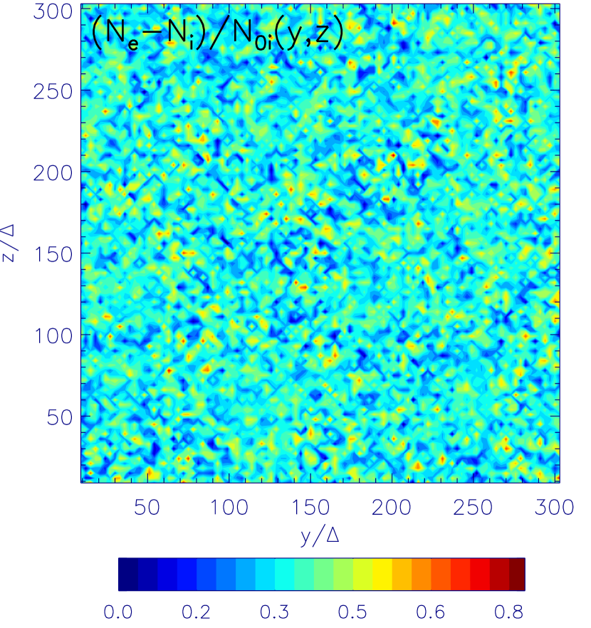
Figure 4: Ambient electron-ion density contrast $N_{e}-N_{i}$ normalized to the initial ion density for run A at $x/\Delta=500$ and $t\simeq 10\gamma_{max}^{-1}$, as in Fig. 5. The average value for the normalized density contrast is $1/3$ on account of the excess electrons that are needed to neutralize the charge carried by the cosmic-ray ions. There are no systematic large-scale deviations from the mean, indicating that the electron and ion density distributions are nearly cospatial.

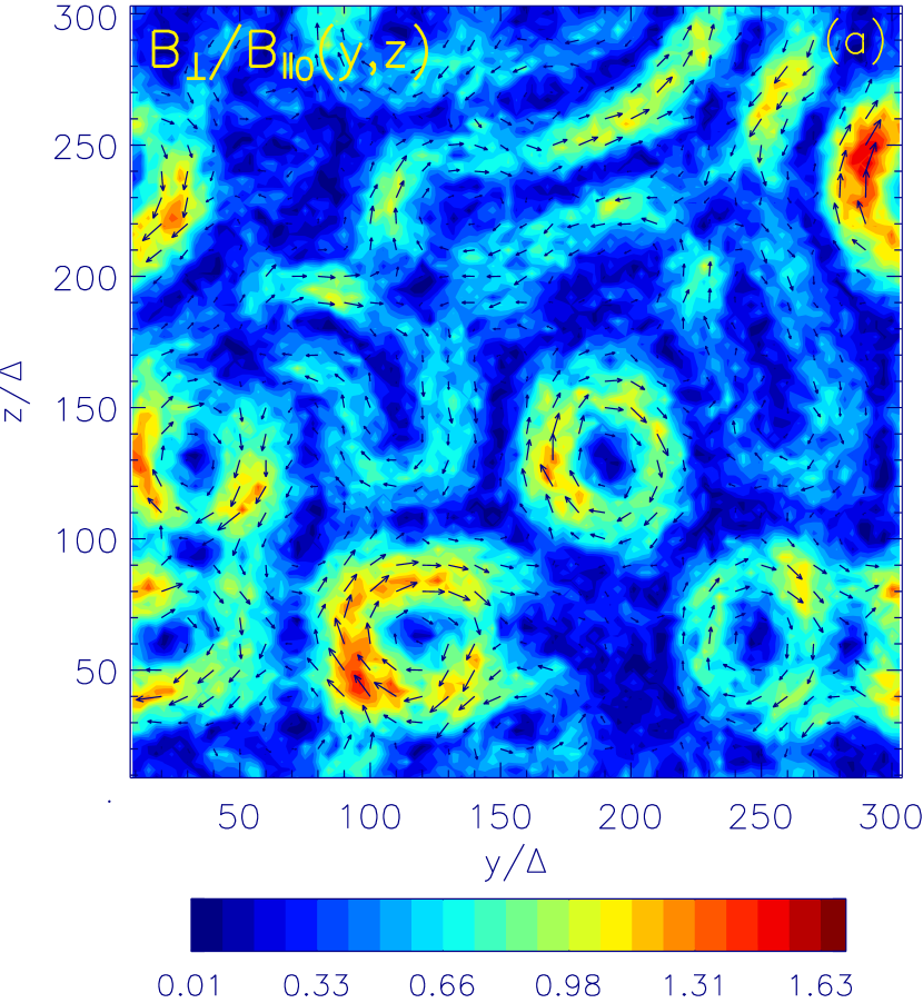
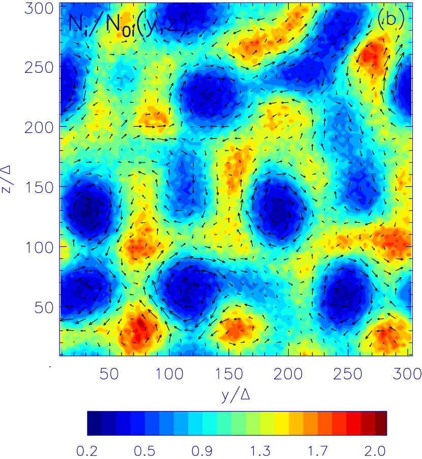
Figure 5: The left panel displays the magnitude and direction, indicated by the arrows, of the perpendicular magnetic field component $B_{\perp}=(B^{2}_{y}+B^{2}_{z})^{1/2}$ in the plane perpendicular to the cosmic-ray drift direction at the grid position $x/\Delta=500$ and time $t\simeq 10\gamma_{max}^{-1}$. $B_{\perp}$ is normalized to the amplitude of the homogeneous field $B_{\parallel 0}$. The right panel shows the density of ambient ions, $N_{i}$, in units of the initial ion density at the same location and time. The electron distribution follows that of ambient ions (see Fig. 4).

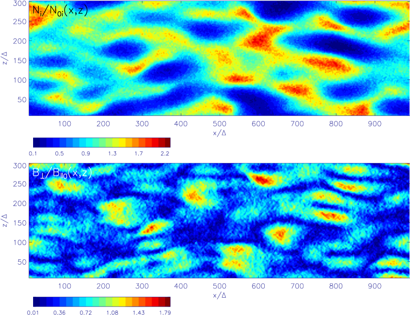
Figure 6: The magnitude and direction of the perpendicular magnetic field component $B_{\perp}=(B^{2}_{y}+B^{2}_{z})^{1/2}$ (bottom panel) and the ambient ion density $N_{i}$ (top panel) in the plane of the cosmic-ray ion drift direction at $y/\Delta=150$ and $t\approx 10\gamma_{max}^{-1}$. A comparison with Fig. 5 illustrates the appearance of oblique filamentary structures.

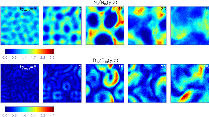
Figure 7: Snapshots of the time evolution of the ion density and the perpendicular magnetic-field component structures in the plane perpendicular to the cosmic-ray ion drift direction at $x/\Delta=500$.

The spatial structure of the turbulent magnetic field and the density of the ambient plasma are shown in Figs. 4, 5, and 6 for $t\approx 10\,\gamma_{max}^{-1}$, and found in the analytical theory Fig. 7 presents snapshots of the temporal evolution of these structures in the plane perpendicular to the cosmic-ray drift direction. To be noted from Fig. 4 is that the density variations of the ambient electrons and ions are nearly cospatial, apart from some variations on small scales that arise largely from statistical fluctuations, so it is sufficient to only show the ion density in Figs. 5, 6, and 7. The background plasma forms filamentary structures of plasma voids surrounded by regions of enhanced plasma density. At any given time, the thickness of these structures, or their separation, corresponds to the $\lambda_{\perp}$ component of the dominant wave mode, and the correlation length along the cosmic-ray streaming direction is equal to $\lambda_{\parallel}$. The cosmic-ray distribution remains homogeneous throughout the duration of the numerical experiment, but the voids become completely depleted of ambient ions and electrons except for the excess electrons which neutralize the charge in cosmic-ray ions. The currents carried by cosmic rays are therefore no longer neutralized, and a strong net current flows inside the filamentary ambient-plasma voids, resulting in magnetic-field lines circling around the center of the cavities according to Ampère’s law. Such filamented current structures with azimuthal magnetic fields and radial electric fields are also observed in other simulations (Nishikawa et al., 2006).

The perpendicular magnetic field is thus concentrated around regions of low background plasma density, but constant cosmic-ray density. In the MHD description, the formation of cavities in the plasma is due to the $\vec{j}_{ret}\times\vec{B}$ force, which accelerates the ambient plasma away from the center of the voids, thus causing the cavities to expand (B04, B05, Milosavljević & Nakar, 2006). In our kinetic simulations, mainly the electrons are subject to this force, since they drift and thus contribute to $\vec{j}_{ret}$. Ambient-ion motion away from the cavities, and a restoring influence on the electrons, is caused by an electrostatic charge-separation field, which is stronger than the original $\vec{j}_{ret}\times\vec{B}$ force for non-relativistic drifts.

3.2 Theoretical Analysis of Current Filament Structure

The formation of the low-density filaments in the ambient plasma can be understood with a simple toy model. We use cylindrical geometry with azimuthal symmetry and assume the cosmic rays to drift homogeneously along the $z$-axis, thus providing a current density $j_{\rm CR}={j_{\rm CR,z}}=e\,N_{\rm CR}\,v_{sh}$. As in our simulations, the ions in the background plasma are at rest and homogeneously distributed with density $N_{i}$, whereas the background electrons are initially homogeneously distributed with density $N_{0e}$ and drift along the $z$-axis with velocity $v_{\rm d}=v_{\rm d,z}=v_{\rm sh}\,N_{\rm CR}/N_{\rm 0e}$ to cancel the cosmic-ray current and charge. Now suppose a small displacement of electrons occurs at some location, so that

$$\delta N_{e}(r)=-N_{0e}\,\eta\,r_{1}\,\left[\delta(r-r_{1})-{{r_{1}}\over{r_{2}}}\,\delta(r-r_{2})\right]$$ (3)

where we assume for simplicity $r_{2}>r_{1}$ and introduce $\eta>0$ as a small perturbation parameter. The displacement breaks the current balance, so that an excess current exists with

$$\delta j_{z}(r)=j_{\rm CR}\,\eta\,r_{1}\,\left[\delta(r-r_{1})-{{r_{1}}\over{r_{2}}}\,\delta(r-r_{2})\right]$$ (4)

This current creates an azimuthal magnetic field that is determined by Ampère’s law. The field is non-vanishing only between $r_{1}$ and $r_{2}$ and has the amplitude

$$B_{\phi}(r)=\mu_{0}\,j_{\rm CR}\,\eta\,{{r_{1}^{2}}\over r}\qquad r_{1}<r<r_{2}$$ (5)

The small displacement of electrons also implies a violation of charge balance, leading to a radial electric field of amplitude

$$E_{r}(r)={{j_{\rm CR}}\over{\epsilon_{0}\,v_{\rm d}}}\,\eta\,{{r_{1}^{2}}\over r}\qquad r_{1}<r<r_{2}$$ (6)

The electric force on the electrons is therefore a factor $c^{2}/v_{\rm d}^{2}\gg 1$ larger than the average magnetic force, so they are accelerated inward. The ambient ions see on average only the electric force, because at least initially they do not drift, which accelerates them outward, albeit with an acceleration much smaller than that of the electrons. The cosmic rays are virtually unaffected on account of their large random velocities, which implies that they see any acceleration only for a very short time. The dominant electric field prevents a separation of ambient ions and electrons, and in fact we see in Fig. 4 that these two particle species are nearly cospatial. The ambient ions and electrons readjust their spatial distributions until charge balance is re-established, but as a bulk they move slightly outward, so the currents are not balanced. Consequently, a current-density profile is established that resembles that described in Eq. 4, although the parameters $\eta$, $r_{1}$, and $r_{2}$ will not be the same as before. Nevertheless, a magnetic field similar to that in Eq. 5 results, that is not compensated by an electric field. The ${\bf v}\times{\bf B}$ force will pull electrons outward and with them the ambient ions, because they are electrostatically bound to the electrons. Reusing Eq. 4 with modified parameters $\eta^{\prime}$, $r_{1}^{\prime}$ and with $\omega_{\rm pi}$ as the ion plasma frequency, the radial acceleration of the ambient plasma can be written as

$$a_{r}(r)=\omega_{\rm pi}^{2}\,r_{1}^{\prime}\,\eta^{\prime}\,{{v_{\rm d}^{2}}\over{c^{2}}}\,{{r_{1}^{\prime}}\over r}=\omega_{\rm pi}^{2}\,r_{1}^{\prime}\,\eta^{\prime}\,{{N_{CR}^{2}}\over{N_{e}^{2}}}\,{{v_{sh}^{2}}\over{c^{2}}}\,{{r_{1}^{\prime}}\over r}$$ (7)

so the growth time can be estimated as

$$t_{\rm filament}\simeq\sqrt{{r_{1}^{\prime}}\over{a_{r}}}={1\over{\sqrt{\eta^{\prime}}\,\omega_{\rm pi}}}\,{{N_{e}}\over{N_{CR}}}\,{c\over{v_{sh}}},$$ (8)

which recovers the scaling of Eq. 2 and is identical to the result of B05 for the filamentary mode. It also shows the same scaling as the expected growth rate of the parallel plane-wave mode (see Eq. 2). For efficiently accelerating SNRs $t_{\rm filament}$ could be of the order of hours or days, if $\eta^{\prime}$ were close to unity.

If the initial displacement of the electrons were inward ($\eta<0$ in Eq. 3), an inward transport of ambient plasma would result. However, the electrostatic restoring force (Eq. 6) would be stronger on account of the $1/r$-profile, and therefore a weaker current imbalance would result after the re-establishment of charge balance in the background plasma, thus imposing a preference for outward displacement of the ambient plasma and the creation of plasma voids.

3.3 Non-linear Evolution of Current Filaments

The expansion of the plasma cavities is visible in Figure 7, and also as the evolution toward larger scales in the power spectra shown in Figs. 2 and 3. The growth of the cavities and the subsequent merging of the adjacent plasma voids lead to a compression of the plasma between cavities and also to an amplification of the magnetic field. Because the magnetic field has a preferred orientation around each cavity, the magnetic field lines may cancel each other in the space between the voids (Fig. 5). The turbulence is almost entirely magnetic and there is no large-scale turbulent electric field structure accompanying the filamentary distribution of ambient plasma and perpendicular magnetic field. The electric fields result from thermal plasma motions, the level of which can be estimated from Figure 4.

Compared with Bell’s MHD studies, the growth of the magnetic perturbations in our kinetic modeling is much slower than calculated for the parallel planar mode. The initial growth rate of the perpendicular-field turbulence is only $\sim 0.2\,\gamma_{max}$ prior to $t\gamma_{max}\approx 7$, and becomes smaller during the later evolution, possibly after nearby plasma cavities have started to merge. In the sense of the toy model discussed in §3.2 (Eq. 8), the perturbation parameter must be small, $\eta^{\prime}\leq 0.1$, or neighboring filaments partially cancel the magnetic field between them. Moreover, the amplitude of the turbulent component never considerably exceeds the amplitude of the regular field. Already after about $20\gamma_{max}^{-1}$, when $\delta B_{\perp}\approx B_{\parallel 0}$, the growth of the turbulence starts to saturate. As shown in Figures 1, 2, and 7, the initial filamentary structure of plasma cavities and surrounding magnetic fields becomes disrupted at this stage, and the turbulence is nearly isotropic and highly non-linear. In the simulation frame, which is the initial rest frame of the ambient ions, the turbulent field structures start to move as a consequence of being embedded in the background plasma which itself starts to drift (see § 3.5). Merging of the magnetic structures leads to further amplification of the magnetic field through compression, but at very slow rate. The peak amplitude of the average turbulent field, $\delta B_{\perp}^{max}\simeq 3.5B_{\parallel 0}$, is reached at $t\gamma_{max}\approx 40$, after which the field starts to dissipate. This is related to the increasing length scales and dissipation of the structures in the ambient-plasma density as evident from Figure 3. The electron and ion distributions become homogeneous, but still evolve nearly cospatially, so that currents produced in this process are weak and thus the gradual decay of the magnetic field is slow.

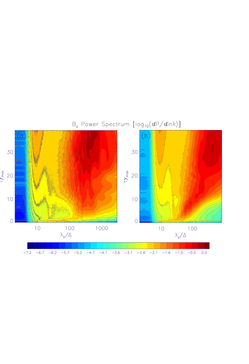
Figure 9: Temporal evolution of the Fourier power spectrum of the magnetic field component $B_{z}$ for run A^∗ (see Fig. 2).

Also clearly visible in Figure 3 is that at $t>25\gamma_{max}^{-1}$ the dominant structures become larger than the size of our simulation box. Using two-dimensional simulations performed on a large computational grid (run A^∗), we have verified that the long-time evolution of the magnetic turbulence and the plasma density fluctuations in the three-dimensional experiment are not considerably influenced by the size of the simulation box. Figure 8 shows the temporal evolution of the energy densities in particles and fields for run A^∗, and Figure 9 presents the power spectrum evolution of the perpendicular magnetic field component. To be noted from the figures is that the initial growth of the perpendicular magnetic field, associated in part with the Buneman-type instability, leads to the higher initial amplitude of the transverse field component in the two-dimensional simulation, and thus $\delta B_{\perp}$ reaches the amplitude of the regular field faster compared with run A. Otherwise, the results of the three-dimensional experiment are qualitatively very well reproduced in the two-dimensional run. At about $t\gamma_{max}\approx 35$ the peak amplitude of the average turbulent field is reached, and its value, $\delta B_{\perp}^{max}\simeq 3.1B_{\parallel 0}$, is very close to that obtained in the three-dimensional simulation. Also, the wavelengths ($\lambda_{\perp}$, $\lambda_{\parallel}$) of the dominant wave mode of the magnetic-field turbulence are numerically similar to those in run A. The dominant turbulent field structures during the late-time evolution are well contained inside the simulation box (Fig. 9), so that the eventual dissipation of the magnetic field is not affected by the boundary conditions.

3.4 Scaling and Parameter Dependence

The question arises to what extent the parameter choice in our simulations influences the plasma dynamics, in particular the turbulence growth rates. We have used the zero-temperature kinetic calculations of Blasi & Amato (2007) to verify that our choice of the reduced ion-electron mass ratio $m_{i}/m_{e}=10$ and a monoenergetic cosmic-ray spectrum with particle Lorentz factor $\gamma_{\rm CR}=2$ has no impact on the growth rate and spatial scale of the instability. For that purpose we have re-evaluated their approximations for $\omega\ll\Omega_{i}^{\ast}$, the nonrelativistic ion gyrofrequency, and as the only impact of our parameter choice we find an additional term in the dispersion relation that scales with the mass ratio. In the notation of Eq. 2 in Blasi & Amato (2007), the dispersion relation would read

$$v_{A}\,k^{2}-{{m_{e}}\over{m_{i}}}\,{{N_{\rm CR}}\over{N_{i}}}\,v_{sh}^{2}\,k^{2}=\omega^{2}\mp{{k\,v_{sh}\,\Omega_{i}^{\ast}\,N_{\rm CR}}\over{N_{i}}}\,\left[1\pm I_{1}(k)\pm\imath\,I_{2}(k)\right]$$ (9)

For a realistic mass ratio and the parameters used by Blasi & Amato (2007), the additional term is negligible, but for the standard parameters in our simulations it is not. In fact, the left-hand side of Eq. 9 is negative for all $k$, and hence for one polarization we find a nearly purely growing solution with a growth rate slightly larger than for $m_{i}/m_{e}=1836$ for all $k\,r_{CRg}\gg 1$ because the functions $I_{1}\ll 1$ and $I_{2}\ll 1$ for those wavenumbers. These calculations suggest that the small growth rate of the non-resonant streaming instability in our simulations is not caused by the reduced ion-electron mass ratio, in line with the results of additional 2-D simulations using more realistic mass ratios (runs B-E), whose results are described below.

Figure 10 shows the temporal evolution of the energy density in electromagnetic fields and particles for a two-dimensional run with $m_{i}/m_{e}=500$ (run E). One can note from the figure and also from Table 1 that the fundamental properties of the magnetic turbulence observed in the three-dimensional experiment (run A) are also seen in the additional simulations for $m_{i}/m_{e}=40,100,150$ and $500$. In particular, for all mass ratios the dominant wave mode, which is the oblique filamentary mode, has approximately the same growth rate, much slower than predicted by the quasi-linear estimates, and a wavevector with the same inclination to the drift direction $\theta\approx 70^{\circ}$. The two-dimensional simulations for high ion-electron mass ratios (runs D and E) also show that the saturation level of the magnetic turbulence is similar to that observed in the three-dimensional experiment with $m_{i}/m_{e}=10$.

Finite-temperature effects in background plasma can limit the growth rate of the non-resonant instability (Reville et al., 2006, 2007). Since our simulations do not exactly reproduce the analytical estimates for the zero-temperature limit, we used the analytical scalings of Reville et al. (2007) to assess the role of the thermal effects. The initial heating of the ambient-particle populations associated with, e.g., the Buneman instability leads to ion temperatures of the order $\Theta=k_{B}T/m_{i}c^{2}\approx 10^{-4}-10^{-3}$. At these temperatures the growth rates for the most unstable wave modes should be reduced as $\gamma_{max}(\Theta=10^{-4})\simeq 0.9\,\gamma_{max}(\Theta=0)$ and $\gamma_{max}(\Theta=10^{-3})\simeq 0.5\,\gamma_{max}(\Theta=0)$. This means that thermal effects alone cannot explain why in our simulations a filamentation mode with a growth rate of $0.2\,\gamma_{max}(\Theta=0)$ is observed, but not the parallel non-resonant mode.

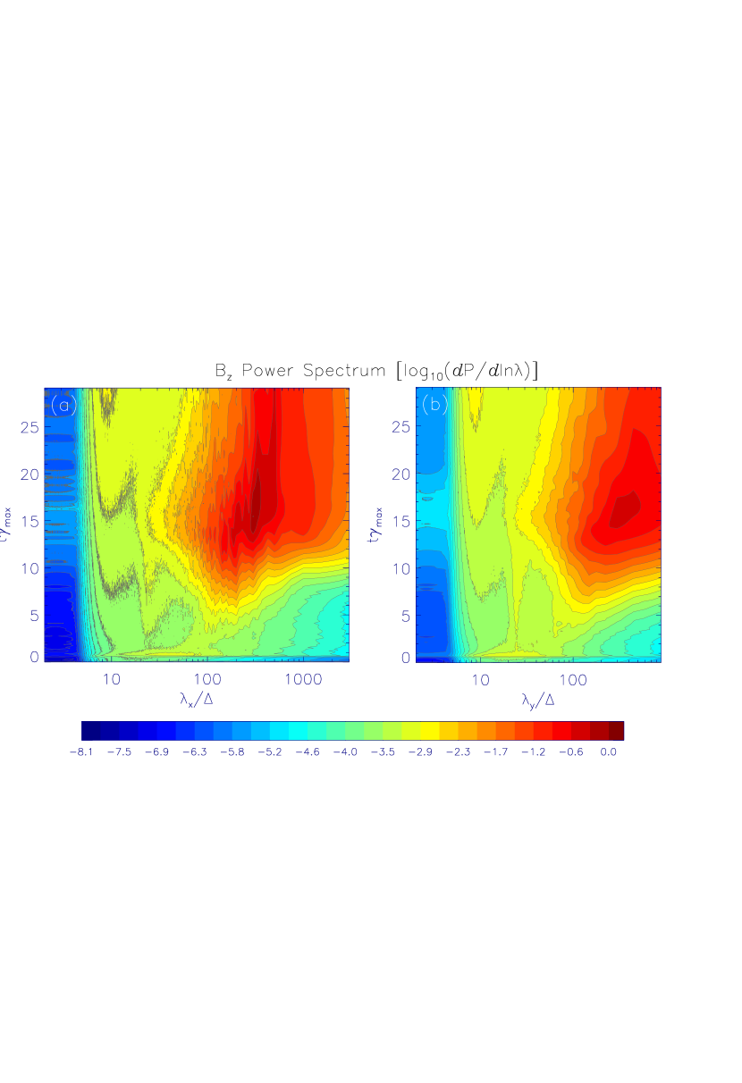
Figure 12: Temporal evolution of the Fourier power spectrum of the magnetic field component $B_{z}$ for run F (see Fig. 2).

For the two-dimensional run F with $m_{i}/m_{e}=10$ we have increased the strength of the regular magnetic field component $B_{\parallel 0}$. In that case the turbulence scales ($\lambda_{max}$) are much better separated from the plasma scales; in fact, $\lambda_{max}$ is a factor of three larger than in the runs A and A^⋆, whereas the electron and ion skindepths are the same as before. In this way we also probe the production of magnetic turbulence in more magnetized upstream plasma, in which the shock is weaker with an Alfvénic Mach number $M_{A}=6.3$. The results are presented in Figures 11 and 12 and summarized in Table 1, where the reader will note that the growth of the turbulence is faster than that for stronger shocks with a maximum rate 0.35 $\gamma_{max}$. However, the saturation level is essentially the same as in all the other simulations. Furthermore, the faster evolution allows us to better follow the late-time behavior of the system, and we clearly observe the turbulent magnetic field to slowly decay until at the end of the simulations the energy density in the turbulent magnetic field is within a factor 2 of that in the homogeneous magnetic field. We conclude that there is no evidence for significant magnetic field amplification, although we do observe a small change in the dominant oblique filamentary mode, which has a wavevector that is slightly better aligned with the drift direction ($\theta=\angle(\vec{k},\vec{v}_{s})\approx 53^{\circ}$), which appears to be a general trend when $\lambda_{max}$ is expected to be a higher multiple of the ion skindepth.

We also performed a number of simulations with reduced $N_{CR}/N_{i}$, for which the expected growth rate of the non-resonant instability decreases according to the quasi-linear estimates. A smaller cosmic-ray current implies that the electrons in the background plasma can compensate that current with a smaller drift velocity, thus lessening the impact of the initial electrostatic Buneman-type instability and the associated heating. The runs G to J therefore involve lower plasma temperatures throughout the duration of each simulation. The growth of the magnetic turbulence becomes very slow in these simulations, which use the same $\delta t\ll\omega_{pe}^{-1}$ as runs A-F, and therefore in run J with $N_{CR}/N_{i}=1/30$ we follow only the initial evolution. The runs G-I are for $N_{CR}/N_{i}=1/10$ and three different magnetizations, implying that the expected turbulence scales, $\lambda_{max}$, are between 2 times and 10 times the ion skindepth. The mass ratio is $m_{i}/m_{e}=50$ for all runs with small density ratios. As in the case of runs A-F, the mean amplitude of the turbulent magnetic field peaks at a few times the homogeneous field strength and we observe an oblique filamentation mode, not the parallel mode expected from quasi-linear theory.

3.5 The Evolution of the Particle Spectra

In all runs a random sample of 0.1% - 0.3% of each particle species (electron, ion, cosmic ray), corresponding to about $10^{6}$ particles, is selected every few hundred timesteps to observe the evolution of the velocity distributions. The average particle velocity is the particles’ drift velocity and is plotted for all three species in Fig. 13 for run A. To be noted from the figure is the disappearance of a relative drift between the cosmic rays and the background ions and electrons: after approximately $40\,\gamma_{max}^{-1}$ all particles drift with approximately the same bulk velocity of about $0.14\,c$. At the same time the turbulent magnetic field reaches its peak energy density, as is shown in Fig. 1. The same basic behavior is seen in the other simulations as well. This finding is in line with the notion that the cosmic-ray drift relative to the background plasma drives the turbulence: as the relative velocity between cosmic rays and plasma decreases, so does the source of the non-resonant streaming instability. We have performed a test simulation (run I^∗ in Table 1), in which we do not allow any acceleration of cosmic rays by increasing their particle mass by a factor $2\times 10^{8}$ and leaving all other parameters as in run I. Indeed, the cosmic-ray drift remains constant and the magnetic field grows to a bit more than twice the amplitude as compared with run I. The background plasma would still experience a bulk acceleration, but now the magnetic-field growth terminates only when the plasma has assumed the full original cosmic-ray drift speed rather than about half of it as in all the other simulations, thus delaying the saturation.

The bulk acceleration of the background plasma plays a key role in shaping cosmic-ray modified shocks, although in realistic SNRs the process must be expected to operate on a timescale similar to that on which the local conditions change on account of the approaching shock. In a steady state the upstream plasma will assume a bulk velocity that is essentially determined by the local density of cosmic rays. In any case one expects a continuous change in the plasma flow velocity, which permits the overall compression ratio between far upstream and far downstream to be much larger than the limit given by the Rankine-Hugoniot jump conditions (e.g. Vladimirov et al., 2006). Our simulations detail how the changes in the bulk-flow properties relate to the average amplitude of the magnetic field.

Besides the buildup of magnetic turbulence and the bulk acceleration of the background plasma we can also study the heating of the plasma, which is of particular interest for models of cosmic-ray acceleration because it limits the sonic Mach number of the shock and hence could reduce the acceleration efficiency. After a Lorentz transformation into the bulk-flow frame of a given plasma component (see Appendix A for details), measurements of the azimuth-integrated particle distribution can reveal anisotropies and spectral evolution. Such an analysis shows that all particle species, cosmic rays as well as the background ions and electrons, remain moderately isotropic in their instantaneous bulk-flow rest frames, but a certain stretching of the distributions along the drift direction is clearly seen. Therefore, care must be exercised in deriving and interpreting the momentum spectra of the particles.

The cosmic rays start the simulation with an isotropic and monoenergetic distribution with Lorentz factor $\gamma_{\rm CR}=2$. During the simulation isotropy is maintained to within 0.5%, and the momentum distribution of the cosmic rays continuously broadens, but remains approximately a Gaussian centered on $mc\sqrt{\gamma_{\rm CR}^{2}-1}$ with a mode that does not change appreciably.

The momentum distributions of the background ions and electrons intermittently develop a high-energy tail, at least part of which can be attributed to anisotropy because the particles in the high-energy tail predominantly move along the drift direction. A more detailed inspection, however, reveals that most of the anisotropies arise from the initial electrostatic Buneman-type instability, because they appear long before the non-resonant magnetic instability sets in. The initial electrostatic instability involves essentially only electric fields parallel to the drift direction which significantly stretch the distributions of slow particles, which is why the background ions are most strongly affected with peak anisotropies of 20%. The Lorentz force contributed by the perpendicular components of the magnetic fields provides re-isotropization which is faster for electrons than for ions on account of the difference in gyrofrequency, but even in the case of the ions the anisotropy is down to $\lesssim\,$3% after about $t\,\gamma_{max}\simeq 15$ in the main three-dimensional simulation.

As outlined in appendix A, we can split the kinetic energy density of particles into the components associated with the bulk motion and the random motion. We denote increases in the random energy density as heating, but the reader should note that this does not necessarily imply a thermalization. Figure 1 shows the temporal evolution of the random energy density for all three particle species in run A. Substantial heating of both the electrons and the ions in the background plasma is observed early in the simulation as a result of the initial electrostatic instability. Further strong heating occurs after $t\,\gamma_{\rm max}\simeq 20$, when the random energy density of all background plasma species is always higher than their bulk energy density. The mean random kinetic energy per particle, or “temperature,” is typically different for the electron and ions in the background plasma. After the initial Buneman-type instability the electrons are hotter, but roughly at the time the filamentation instability has taken over and turned non-linear, the ions are strongly heated and they eventually become hotter than the electrons. These results on the anisotropy and heating are seen in the main three-dimensional simulation, but qualitatively the same behavior is observed also in two-dimensional runs.

If the observed heating of the background plasma were real, then the upstream medium of an SNR forward shock would be so hot that the forward shock itself could be only very weak, if it existed at all. There are reasons to assume that our simulations for technical reasons overestimate the heating, and therefore we cannot make firm statements on the temperature of a real plasma upstream of SNR shocks with efficient particle acceleration. One reason is that we must limit the number of simulated particles to simulate the long-term evolution in large simulation boxes. Statistical fluctuations then give rise to small-scale electric fields that heat the plasma. A short test simulation with large particle number (160 per cell in total) was performed and indeed the plasma temperature was observed to be somewhat reduced, although the ions eventually reached a temperature similar to that observed for smaller particle number. As statistical fluctuations are suppressed only with $\sqrt{N}$, simulations with low density ratio and a sufficiently large number of particles per cell are prohibitively expensive, even in two dimensions. Other computational techniques like $\delta f$-PIC simulations (Sydora, 1999) may be better suited for that purpose.

Also, a substantial part of the initial heating and small-scale electric fields is related to the initial electrostatic Buneman-type instability, the effect of which depends on the drift velocity of the background electrons. Because the electrons carry the return current that compensates the cosmic-ray current, their drift velocity is $v_{d}=v_{sh}N_{CR}/N_{e}$. We must keep the shock speed $v_{sh}$ (the cosmic-ray drift velocity) high to enable a sufficiently fast growth of the non-resonant streaming instability. We can vary the density ratio $N_{CR}/N_{e}$ somewhat using particle splitting, but that also adversely affects both the growth rate and the wavelength of the non-resonant streaming instability. We have run three test simulations with $N_{CR}/N_{i}=1/10$ and one with $N_{CR}/N_{i}=1/30$ to further explore this issue. We find that the plasma temperature, or more precisely the average random kinetic energy per particle, is indeed significantly reduced by about an order of magnitude throughout the simulation. Nevertheless, the buildup of magnetic turbulence is unchanged compared with the earlier experiments. The plasma temperature is still unrealistically high, probably on account of heating in small-scale electric fields that arise from statistical charge-density fluctuations.

4 Summary and Discussion

4.1 Summary of Our Results

The generation of magnetic-field turbulence by cosmic-ray ions drifting upstream of SNR shocks has been studied using two- and three-dimensional PIC simulations for a variety of parameters. Turbulent field is indeed generated in this process, but the growth of magnetic turbulence is slower than estimated in the literature, and the turbulence is of a different nature: we observe a modified filamentation of the ambient plasma, but not the cosmic rays, in contrast to the parallel wave found in quasi-linear calculations. The filamentation and formation of cavities in the background plasma was also observed in recent MHD simulations.

The amplitude of the field perturbations saturates at approximately the amplitude of the homogeneous upstream field. The energy density in the turbulent field is also always much smaller than the plasma kinetic energy density. This suggests that the efficiency of magnetic-field generation through this mechanism may not be sufficient to account for the strong magnetic-field amplification invoked for some young SNRs and also leaves open the question whether or not diffusive particle acceleration at SNR shocks can produce particles with energies beyond the “knee” in the cosmic-ray spectrum.

The backreaction of the magnetic turbulence on the particles leads to an alignment of the bulk flow velocities of the cosmic rays and the background medium in all our simulations. This is precisely what is making up a cosmic-ray modified shock: the upstream flow speed is continuously changed by the cosmic rays, so the compression ratio of the actual shock of the thermal plasma is moderate, whereas the overall compression ratio can be large. The new and surprising result of our simulations is that we accomplish this without significant magnetic-field amplification and with instability modes different from those invoked for the purpose in the recent literature.

4.2 Comparison with Published MHD Simulations

How can we understand the differences between the results of the analytical solutions, the MHD simulations, and our PIC study? First of all, not too much is different: the filamentation mode observed in our simulations is similar to the cylindrical filamentary mode that was analytically described in B05 and in its evolved, then isotropic form observed in the MHD simulations of B04, B05, Z08, Reville et al. (2008a). The growth rate, or expansion rate, of the filaments is somewhat smaller than expected for isolated filaments, probably because neighboring filaments produce between them magnetic fields of opposite orientation, thus cancelling part of the magnetic field that one would calculate for an isolated current filament. We do not observe a filamentation of the cosmic rays, probably because throughout the simulations the cosmic-ray Larmor radius, $r_{CRg}$, remains larger than the spatial scale of the magnetic turbulence. As we observe the magnetic-field growth to saturate and the cosmic-ray drift relative to the background plasma to disappear, there is no significant cosmic-ray current remaining that could initiate a further amplification of the magnetic field at later times, beyond the termination of our simulations.

The MHD simulations of B04, B05, and Z08 show the magnetic-field growth to an amplitude much higher than the initial homogeneous field. However, they assume the cosmic-ray current to be constant throughout the simulations. In our study the cosmic-ray current changes and is strongly reduced in the non-linear phase, when the magnetic-field growth saturates. Because in the MHD simulations the cosmic-ray current is constant in time and uniform in space, these simulations consequently cannot capture this backreaction. In the test run I^∗ (see §3.5 and Table 1), in which the backreaction of cosmic rays has been excluded by increasing cosmic-ray particle mass, we observe the peak in the average magnetic-field strength more than a factor 2 higher than with cosmic-ray backreaction (run I). In this test simulation the saturation of the field amplification arises from the bulk acceleration of the ambient plasma which is still permitted. In the MHD simulations, it is unclear to what extent momentum is transferred to the background plasma, but in any case that process is likely suppressed because the energy and momentum flux of the cosmic rays is not accounted for.

B04, B05, and Z08 describe the magnetic-field structure in the MHD simulations at various stages of the evolution. The non-linear turbulence appears fairly isotropic and bears some resemblance to the structure shown in Figs. 5 and 7, although the MHD results reveal no structures visibly extended in the drift direction. The MHD simulations show much more structure on the smallest scales, most of which are prominent at late stages when the turbulence in our PIC simulations has already saturated. The one-dimensional spectra of the perpendicular magnetic field in the MHD simulation of Z08 indicate strong growth on all spatial scales after the turbulent field becomes stronger than about 10% of the homogeneous field. From that time on the velocity fluctuations in the background plasma are also of the same order as, if not stronger than, the adiabatic sound speed, indicating that weak shocks can be formed. In our simulations shocks would be resolved, which may explain why the MHD simulations show more structures on the smallest scales.

The discussions in B04, B05, and Z08 do not indicate that a parallel planar mode is indeed initially observed in the MHD simulations. Also, neither magnetic-field spectra in $k_{\perp}$ nor spectra of the parallel component of the magnetic field are presented. Our discussion of the differences between the results of these MHD simulations and our PIC study must therefore remain limited in scope. We stress, however, that the saturation of the turbulence growth in our simulations arises from the backreaction of the magnetic field on the bulk velocities of cosmic rays and background plasma. The higher magnetic-field saturation level in the MHD simulations is most likely a direct result of the assumption of a constant cosmic-ray current. A strong magnetic-field amplification to amplitudes $\delta B\gg B_{0}$ has yet to be demonstrated.

4.3 Comparison with Analytical Calculations

The turbulence observed in our simulations reflects analytical results for filamentation modes, e.g., the derivation by B05. A discrepancy only exists as far as the parallel plane-wave mode is concerned. All published analytical calculations agree that in quasi-linear treatment a parallel, purely growing mode should dominate. What might be the reasons why we do not see this mode in our PIC simulations? We have already determined that the plasma temperature is probably not responsible for this discrepancy. One possibility is that the mode exists initially, but is invisible in the noise, and changes its character quickly so that we observe the filamentation, which was already described in B05. In fact, the parallel plane-wave mode and the filamentation of the ambient plasma are expected to show a similar growth rate. This interpretation would be in line with the magnetic-field structure observed in the MHD simulations before the turbulent magnetic field reaches the amplitude of the homogeneous field, $B_{\parallel 0}$, which also does not clearly show a parallel mode.

The most likely reason is that our choice of parameters may not reflect one of the assumptions made in the analytical treatments, namely that the frequency of the perturbations be much smaller than the ion gyrofrequency (e.g. Reville et al., 2007), whereas we typically have to choose parameters for which the theoretically expected growth rate is similar to the ion gyrofrequency, i.e. $\Im\omega\approx\Omega_{i}$. According to the quasi-linear results,

$${{\Im\omega}\over{\Omega_{i}}}\approx{{v_{sh}\,N_{CR}}\over{2\,V_{A}\,N_{i}}}\ ,$$ (10)

implying that if either the shock speed or the cosmic-ray density is too high, the assumption of a small frequency is no longer justified, and the character of the instability may be different. However, the observed growth rate of the filamentation mode in our simulations is an upper limit to the growth rate of any parallel mode that we do not see, so in fact all our simulations have an observed growth rate $\Im\omega_{obs}\lesssim 0.3\,\Omega_{i}$ and some simulations show $\Im\omega_{obs}<0.2\,\Omega_{i}$.

If $\Im\omega\ll\Omega_{i}$ must be strictly maintained, then what are the constraints on the parameters so the parallel plane-wave mode can play a role? Assuming efficient Bohm-type diffusion, the upstream plasma is swept up by the shock on a timescale $c\,r_{CRg}/3\,v_{sh}^{2}$, so efficient growth requires the growth time be substantially smaller than this:

$$1\gg{{\Im\omega}\over{\Omega_{i}}}\gg\ {{3\,\beta_{sh}^{2}}\over\sqrt{\gamma_{CR}^{2}-1}}.$$ (11)

If conditions allow a rapid growth of the instability on a timescale much shorter than the shock-capture timescale, meaning if the instability is astrophysically relevant, then the instability will also evolve in an environment that is essentially not changed by the inflow of fresh material, implying that our simulation setup using periodic boundary conditions on all sides is appropriate.

For young SNRs the forward-shock speed is $\beta_{sh}\gtrsim 0.01$, so that only a narrow range of interesting parameters exists, unless we consider very high-energy cosmic rays for which the instability-driving current is small. We can use Eq. 10 to rewrite the second relation in Eq. 11 using $U_{CR}\simeq N_{CR}\,\sqrt{\gamma_{CR}^{2}-1}\,m_{i}\,c^{2}$ as the cosmic-ray energy density, and $U_{bulk}={1\over 2}\,N_{i}\,m_{i}\,v_{sh}^{2}$ as the bulk kinetic energy density of the upstream plasma:

$$U_{CR}\gg 12{{v_{A}}\over{v_{sh}}}\,U_{bulk}\approx 0.1\,U_{bulk}.$$ (12)

Here the second relation applies to SNRs with small upstream plasma density $N_{i}\lesssim 0.1\ {\rm cm^{-3}}$, such as SN 1006, RX J1713-3946, or Vela Junior, for which the Alfvén speed is $v_{A}\simeq 30$ km/s for a reasonable magnetic-field strength $B_{0}\simeq 5\ \mu$G. It is unlikely that the energy density in cosmic rays is much larger than the bulk energy density of the upstream plasma, suggesting that this instability can operate for only a few e-folding times in those SNRs. Remnants that expand into a high-density environment may be better suited for a strong growth of the non-resonant mode, but in those cases one has to consider ion-neutral collisions which can reduce the growth of the instability (Reville et al., 2008b).

The relation Eq. 12 may be a more severe constraint than the requirement

$$k_{\parallel max}\,r_{CRg}=\frac{\zeta}{2}\frac{v_{sh}^{2}}{v_{A}^{2}}={{U_{CR}}\over{U_{bulk}}}\,{{v_{sh}^{3}}\over{2\,c\,v_{A}^{2}}}\gg 1$$ (13)

for the instability to exist in the first place (compare Eq. 1), and should be used in addition to it. Equation 12 also shows that cosmic rays of very high energy are not necessarily better triggers of magnetic-field amplification. The relevance of cosmic rays in a certain energy band primarily depends on the energy density they carry.

Our simulations used cosmic rays with a moderate Lorentz factor $\gamma_{CR}=2$. It may be interesting to speculate how our results might change, had we been able to use a substantially higher cosmic-ray Lorentz factor, e.g., $\gamma_{CR}=1000$. A spatial re-organization of the cosmic rays was not observed in our simulations, and higher-energy particles are more difficult to concentrate in certain locations, so the homogeneity of the cosmic-ray distribution would most likely not change. Leaving the energy density in cosmic rays unchanged, we would expect a much slower growth of turbulence on much larger scales. The condition $\Im\omega\ll\Omega_{i}$ should always be on account of the small number of cosmic rays required to carry their energy density (see Eq. 10), and so the parallel mode should be initially excited and then give way to the filamentation and formation of cavities that was observed in the MHD simulations and our PIC studies. For the backreaction and saturation we therefore do not expect fundamental deviations from the behavior that we saw in our simulations. We studied systems with turbulence growth on a variety of scales relative to the plasma scale, and we never saw a systematic variation in the saturation mechanism and level, that might indicate a dependence on the wavelength of the turbulence. Even though we could not possibly study a system with, e.g., TeV-ish cosmic rays, we therefore feel there is no reason to assume that in such a situation the bulk acceleration of the plasma and the cosmic rays would proceed in a different way. The saturation level of the turbulent magnetic field would then also be similar to what we find. What remains unclear is the actual equilibrium amplitude in a realistic astrophysical scenario, in which the instabilities operate under a competition of saturation through non-linear backreactions with driving through the influx of fresh material. Since the saturation level observed in our simulations corresponds to a situation in which the backreactions are relatively fast, also compared with the initial growth, it appears likely that even under continuous inflow of new plasma the equilibrium amplitude of the turbulent magnetic field does not exceed the peak values seen in the PIC simulations, so that $\delta B/B\sim 1$ remains the most probably result.

Appendix A Transformations of the Particle Distributions and their Momenta

It is convenient to use cylindrical phase-space coordinates $p_{\parallel}$, $p_{\perp}$, and $\phi$, where the differential volume element is $d^{3}p=dp_{\parallel}\,dp_{\perp}\,p_{\perp}d\phi=\frac{1}{2}dp_{\parallel}\,dp_{\perp}^{2}\,d\phi$, with the axial component $p_{\parallel}$ defined, in this case, by the direction of a Lorentz transformation. In our discussion the azimuthal angle can be ignored, so it is sufficient to consider gyrotropic distribution functions

$$f(p_{\parallel},p_{\perp})={1\over\pi}\,{{dn}\over{d^{3}x\,dp_{\parallel}\,dp_{\perp}^{2}}}.$$ (A1)

If the distribution function is known in some inertial reference frame $K$, then in a second reference frame $K^{\prime}$ moving at velocity $\beta\,c\,{\bf e_{\parallel}}$ with respect to $K$, the density, bulk velocity, and total energy density of the particles are given by

$$n^{\prime} \equiv \int d^{3}p^{\prime}\ f^{\prime}\left({\bf p^{\prime}}\right)$$ (A2)

$${\bf V^{\prime}} \equiv \frac{1}{n^{\prime}}\int d^{3}p^{\prime}\ {\bf v^{\prime}}\,f^{\prime}\left({\bf p^{\prime}}\right)$$ (A3)

$$w^{\prime} \equiv \int d^{3}p^{\prime}\ E^{\prime}\,f^{\prime}\left({\bf p^{\prime}}\right),$$ (A4)

where primed quantities are measured in frame $K^{\prime}$. We exploit the invariance of $f$ and $p_{\perp}$ under the Lorentz transformation to rewrite Eq. A2 as

$$n^{\prime}=\pi\,\int\limits_{-\infty}^{\infty}dp^{\prime}_{\parallel}\int\limits_{0}^{\infty}dp^{2}_{\perp}\ f\left(p_{\parallel}\left(p^{\prime}_{\parallel}\right),p_{\perp}\right).$$

By the appropriate change of coordinates, the effect of the Lorentz transformation can be confined to the Jacobian of the coordinate transformation:

$$n^{\prime}=\pi\,\int\limits_{-\infty}^{\infty}dp_{\parallel}\ \int\limits_{0}^{\infty}dp^{2}_{\perp}\ f\left(p_{\parallel},p_{\perp}\right)\,\left|\frac{dp^{\prime}_{\parallel}}{dp_{\parallel}}\right|_{p_{\perp}=\rm const}.$$ (A5)

Now $p^{\prime}_{\parallel}=\gamma\,\left(p_{\parallel}-\beta\,\frac{E\left({\bf p}\right)}{c}\right)$, where $E\left({\bf p}\right)\equiv\sqrt{m^{2}c^{4}+\left(p^{2}_{\parallel}+p^{2}_{\perp}\right)c^{2}}$. Then the Jacobian is

$$\left|\frac{dp^{\prime}_{\parallel}}{dp_{\parallel}}\right|_{p_{\perp}=\rm const.}=\gamma\,\left(1-\frac{\beta\,c}{E\left({\bf p}\right)}p_{\parallel}\right).$$ (A6)

If we consider a particle distribution that is isotropic, homogeneous, and monoenergetic with scalar momentum $p_{0}$ and density $n$ in frame $K$,

$$f\left({\bf p}\right)=\frac{n}{2\pi p_{0}}\delta\left(p_{\parallel}^{2}+p_{\perp}^{2}-p_{0}^{2}\right),$$ (A7)

we will find that $n^{\prime}=\gamma\,n$. The Jacobian must also be used when setting up the simulations, because in their flow frame cosmic rays are supposed to follow a distribution according to Eq. A7, which must be transformed into the simulation frame, which is the upstream rest-frame ahead of the SNR shock.

We can compute the bulk velocity (Eq. A3) in a similar manner; we express the particle velocity ${\bf v^{\prime}}$ in terms of the integration variables, and only the parallel component $v^{\prime}_{\parallel}$ will survive integration. Now $v^{\prime}_{\parallel}=(v_{\parallel}-\beta\,c)/(1-\beta\,v_{\parallel}/c)$, and $v_{\parallel}=p_{\parallel}\,c^{2}/E$. Then for isotropic and monoenergetic particles (Eq. A7) we may write Eq. A3 as

$${\bf V^{\prime}}={\bf e_{\parallel}}\frac{\pi\,c}{\gamma\,n}\int\limits_{-\infty}^{\infty}dp_{\parallel}\ \int\limits_{0}^{\infty}dp^{2}_{\perp}\ \frac{p_{\parallel}\,c-\beta\,E}{E-\beta\,p_{\parallel}\,c}\,f\left(p_{\parallel},p_{\perp}\right)\,\left|\frac{dp^{\prime}_{\parallel}}{dp_{\parallel}}\right|_{p_{\perp}=\rm const}.$$ (A8)

When Eq. A8 is solved with the appropriate substitutions (Eqs. A6 and A7), the bulk velocity is found to be

$${\bf V^{\prime}}=-\beta\,c\,{\bf e_{\parallel}}.$$ (A9)

Thus the velocity for the Lorentz transformation to the rest frame $K$ of the particle distribution is equal to the bulk, or drift, velocity of the particles in another frame $K^{\prime}$, such as the simulation frame. The particle distributions are not necessarily isotropic in any frame of reference, but Eq. A8 nevertheless allows us to properly calculate the drift velocity of a particle population and to transform the particle distribution into the flow rest-frame, so that the anisotropy properties can be investigated. We can also distinguish bulk and random momentum, and the transformed distribution function in the flow rest-frame gives the particle distribution in random momentum that carries information on heating of the particles and any deviations from the initially prescribed Maxwellians for the background plasma and monoenergetic distributions for the cosmic rays.

The total energy density $w^{\prime}$ is easy to calculate as well, but it is useful to separate it into rest-mass, random and bulk kinetic energy densities as $w^{\prime}\equiv n^{\prime}\,m\,c^{2}+U^{\prime}_{\rm ran}+U^{\prime}_{\rm bulk}$. For simplicity we define them as $U^{\prime}_{\rm ran}\equiv(w^{\prime}/\gamma)-n^{\prime}\,m\,c^{2}$ and $U^{\prime}_{\rm bulk}\equiv(\gamma-1)\,w^{\prime}/\gamma$, as a more detailed calculation would yield for an isotropic distribution. Fig. 1 shows the random and bulk kinetic energy densities (without primes) for the main three-dimensional experiment, run A. Note that the drift velocities, and hence $\gamma$, continuously change throughout the simulation.

Figure 1: For the main three-dimensional simulation (run A) using ion-electron mass ratio $m_{i}/m_{e}=10$, we show the temporal evolution of the average energy density in electromagnetic fields (left panel) and particles (right panel), both normalized to the initial total kinetic energy in the system, $U_{k0}$. Time is in units of the inverse growth rate $\gamma_{max}^{-1}$ for the most unstable mode as predicted in the analytical theory (Eq. 2). $B^{2}_{\perp}$ and $E^{2}_{\perp}$ indicate the magnetic and electric field energy densities in the components perpendicular to the cosmic-ray ion drift direction, i.e. $\langle B_{y}^{2}+B_{z}^{2}\rangle/(2\mu_{0})$ and correspondingly for the electric field. $B^{2}_{\parallel}$, $\delta B^{2}_{\parallel}$, and $E^{2}_{\parallel}$ are defined analogously, where $\delta B^{2}_{\parallel}$ involves only the turbulent component. In the right panel, the total energy density of cosmic rays, ambient electrons, and ions is split into bulk and random components as outlined in Appendix A. The total kinetic energy density in cosmic-ray ions, $U_{CR}$, and its components are scaled by a factor of 10. For comparison, the right panel also shows the time evolution of the volume-averaged magnetic energy density, $U_{M}=\langle B_{x}^{2}+B_{y}^{2}+B_{z}^{2}\rangle/(2\mu_{0})$.

Figure 8: Temporal evolution of the total energy density in electromagnetic fields and particles for run A^∗ (see Fig. 1).

Figure 10: Temporal evolution of the total energy density in electromagnetic fields and particles for the two-dimensional simulation with a realistic mass ratio $m_{i}/m_{e}=500$ (run E; see Fig. 1).

Figure 11: Temporal evolution of the total energy density in electromagnetic fields and particles for the two-dimensional simulation assuming $\lambda_{max}=150$ and $m_{i}/m_{e}=10$ (run F; see Fig. 1).

Figure 13: The time evolution of the bulk (average) velocity of all particle species for run A.

Table 1: Simulation Parameters and Results

Run	Grid	$t^{max}$	$m_{i}/m_{e}$	$N_{i}/N_{CR}$	$\lambda_{si}$	$\lambda_{max}$	$v_{sh}/v_{A}$	$\omega_{pe}/\Omega_{e}$	$\gamma_{max}/\omega_{pe}$	$\gamma/\gamma_{max}$	$\theta$	$\delta B_{\perp}^{max}/B_{\parallel 0}$
	($\Delta^{3}$)	($\gamma_{max}^{-1}$)			($\Delta$)	($\Delta$)					(∘)
A	992$\times$304$\times$304	48.9	10	3	25.3	50	19.1	22.1	0.0137	0.2	79	3.43
A∗	3000$\times$900$\times$3	39.1	10	3	25.3	50	19.1	22.1	0.0137	0.2	79	3.16
B	992$\times$400$\times$400	10.5	40	3	50.7	100	19.3	11.6	0.0069	0.12	62	-
C	992$\times$400$\times$400	16.3	150	3	98.2	200	18.7	5.8	0.0035	0.06	68	-
D	3000$\times$900$\times$3	49.5	100	3	80.8	150	20.3	7.8	0.0043	0.2	73	4.59
E	3000$\times$1500$\times$3	44.9	500	3	180.8	360	18.9	3.3	0.0019	0.23	68	4.43
F	3000$\times$900$\times$3	29.4	10	3	25.3	150	6.3	7.4	0.0137	0.35	53	2.07
G	3200$\times$3000$\times$3	72.1	50	10	51.9	100	65.3	31.9	0.002	0.09	80	8.1
H	3200$\times$3000$\times$3	24.5	50	10	51.9	300	21.8	10.6	0.002	0.58	53	4.1
I	3200$\times$3000$\times$3	23.3	50	10	51.9	500	13.1	6.4	0.002	0.75	39	3.3
I∗	2400$\times$2400$\times$3	20.8	50	10	51.9	500	13.1	6.4	0.002	0.75	39	7.5
J	3200$\times$3000$\times$3	11.7	50	30	51.9	500	43.5	21.3	0.0006	0.7	45	-

Note. — Parameters and selected results of the simulation runs described in this paper. Listed are: the system size $(x\times y\times z)$ in units of the grid cell size $\Delta$, the run duration $t^{max}$ in units of $\gamma_{max}^{-1}$, the ion-electron mass ratio $m_{i}/m_{e}$, the density ratio of ambient ions and cosmic rays, the ion skindepth $\lambda_{si}$ in units of $\Delta$, the wavelength of the theoretically expected most unstable mode $\lambda_{max}$ (in units of $\Delta$, see Eq. 2), the Alfvénic Mach number $M_{A}=v_{sh}/v_{A}$ of the shock, the plasma magnetization as given by the electron plasma to cyclotron frequency ratio, the maximum growth rate $\gamma_{max}/\omega_{pe}$ (see Eq. 2), the actual measured growth rate $\gamma$ in units of $\gamma_{max}$, the obliqueness $\theta=\angle(\vec{k},\vec{v}_{s})$ in degrees of the actual dominant turbulence mode, and the maximum amplitude of the perpendicular magnetic-field perturbations $\delta B_{\perp}^{max}$ relative to the homogeneous magnetic field.

References

- Bell (1978) Bell, A.R. 1978, MNRAS, 182, 443
- Bell (2004) Bell, A.R. 2004, MNRAS, 353, 550, (B04)
- Bell (2005) Bell, A.R. 2005, MNRAS, 358, 181, (B05)
- Bell & Lucek (2001) Bell, A.R., Lucek, S.G. 2001, MNRAS, 321, 433
- Birdsall & Langdon (2005) Birdsall, C. K., & Langdon, A. B. 2005, Plasma Physics via Computer Simulation (6th ed.; IOP Publishing Ltd)
- Blasi & Amato (2007) Blasi, P., & Amato, E., Proc. 30th ICRC, (astro-ph/0706.1722)
- Bret et al. (2005) Bret, A., Firpo, M.-C., & Deutsch, C. 2005, PRL, 94, 115002
- Bret et al. (2007) Bret, A., Gremillet, L., & Bellido, J. C. 2007, Phys. Plasmas, 14, 032103
- Buneman (1993) Buneman, O. 1993, in Computer Space Plasma Physics: Simulation Techniques and Software, Eds.: Matsumoto & Omura, Tokyo: Terra, p.67
- Bykov & Toptygin (2005) Bykov, A.M., Toptygin, I.N. 2005, Astron. Lett. 31-11, 748
- Dieckmann et al. (2008) Dieckmann, M.E., Bret, A., and Shukla, P.K. 2008, New J. Phys., 10, 013029
- Ellison & Vladimirov (2008) Ellison, D.C., Vladimirov, A. 2008, ApJ, 673, L47
- Giacalone (2005) Giacalone J. 2005, ApJ, 624, 765
- Giacalone & Jokipii (1996) Giacalone J., Jokipii, J.R. 1996, JGR, 101, 11095
- Lagage & Cesarsky (1983) Lagage P.O., Cesarsky, C.J. 1983, A&A, 125, 249
- Lazar et al. (2007) Lazar, M., Schlickeiser, R. Shukla, P. K., & Smolyakov, A. 2007 Plasma Phys. Control. Fusion, 49, 1661
- Lucek & Bell (2000) Lucek, S.G., Bell, A.R. 2000, MNRAS, 314, 65
- Malkov & Diamond (2001) Malkov, M.A., Diamond, P.H. 2001, Phys. Plas., 5, 2401
- Marcowith et al. (2006) Marcowith, A., Lemoine, M., Pelletier, G. 2006, A&A, 453, 193
- Milosavljević & Nakar (2006) Milosavljević, M., & Nakar, E. 2006, ApJ, 651, 979
- Nishikawa et al. (2006) Nishikawa, K.-I., Hardee, P. E., Hedadal, C. B., & Fishman, G. J. 2006, ApJ, 642, 1267
- Pelletier et al. (2006) Pelletier, G., Lemoine, M., Marcowith, A. 2006, A&A, 453, 181
- Reville et al. (2006) Reville, B., Kirk, J. G., & Duffy, P. 2006, Plasma Phys. Control Fusion, 48, 1741
- Reville et al. (2007) Reville, B., Kirk, J. G., Duffy, P., & O’Sullivan, S. 2007, A&A, 475, 435
- Reville et al. (2008a) Reville, B., O’Sullivan, S., Duffy, P., & Kirk, J. G. 2008a, MNRAS, 386, 509
- Reville et al. (2008b) Reville, B., Kirk, J. G., Duffy, P., & O’Sullivan, S. 2008b, contributed talk at the workshop: High Energy Phenomena in Relativistic Outflows (HEPRO), Dublin, 24-28 September 2007, arXiv:0802.3322v1
- Sydora (1999) Sydora, R.D. 1999, J. Comp. Appl. Math., 109, 243
- Umeda et al. (2003) Umeda, T., Omura, Y., Tominaga, T., & Matsumoto, H. 2003, Comp. Phys. Comm., 156, 73
- Vladimirov et al. (2006) Vladimirov, A., Ellison, D.C., Bykov, A. 2006, ApJ, 652, 1246
- Zirakashvili et al. (2008) Zirakashvili, V.N., Ptuskin, V.S., Völk, H.J. 2008, ApJ, in press, (astro-ph/0801.4486) (Z08)