Center-to-Limb Variation of Solar 3-D Hydrodynamical Simulations

Abstract

We examine closely the solar Center-to-Limb variation of continua and lines and compare observations with predictions from both a 3-D hydrodynamic simulation of the solar surface (provided by M. Asplund and collaborators) and 1-D model atmospheres. Intensities from the 3-D time series are derived by means of the new synthesis code Ass$\epsilon$t, which overcomes limitations of previously available codes by including a consistent treatment of scattering and allowing for arbitrarily complex line and continuum opacities. In the continuum, we find very similar discrepancies between synthesis and observation for both types of model atmospheres. This is in contrast to previous studies that used a “horizontally” and time averaged representation of the 3-D model and found a significantly larger disagreement with observations. The presence of temperature and velocity fields in the 3-D simulation provides a significant advantage when it comes to reproduce solar spectral line shapes. Nonetheless, a comparison of observed and synthetic equivalent widths reveals that the 3-D model also predicts more uniform abundances as a function of position angle on the disk. We conclude that the 3-D simulation provides not only a more realistic description of the gas dynamics, but, despite its simplified treatment of the radiation transport, it also predicts reasonably well the observed Center-to-Limb variation, which is indicative of a thermal structure free from significant systematic errors.

1 Introduction

A few years back, it was realized that one of the most ’trusted’ absorption lines to gauge the oxygen abundance in the solar photosphere, the forbidden [OI] line at $\lambda$6300, was blended with a Ni I transition. These two transitions overlap so closely that only a minor distortion is apparent in the observed feature. Disentangling the two contributions with the help of a 3-D hydrodynamical simulation of surface convection led us to propose a reduction of the solar photospheric abundance by $\sim$ 30% (Allende Prieto et al., 2001). Using the same solar model, subsequent analysis of other atomic oxygen and OH lines confirmed the lower abundance, resulting in an average value $\log\epsilon$ (O)$=8.66\pm 0.05$ (Asplund et al., 2004).

This reduction in the solar O/H ratio, together with a parallel downward revision for carbon (Allende Prieto et al., 2002; Asplund et al., 2005b), ruins the nearly perfect agreement between models of the solar interior and seismological observations (Bahcall et al., 2005; Delahaye & Pinsonneault, 2006; Lin et al., 2007). A brief overview of the proposed solutions is given by Allende Prieto (2007). Interior and surface models appear to describe two different stars.

Supporters of the new hydrodynamical models, and the revised surface abundances, focus on their strengths: they include more realistic physics, and are able to reproduce extremely well detailed observations (oscillations, spectral line asymmetries and net wavelength blueshifts, granulation contrast and topology). Detractors emphasize the fact that the new models necessarily employ a simplified description of the radiation field and they have not been tested to the same extent as classical 1-D models. The calculation of spectra for 3-D time-dependent models is a demanding task, which is likely the main reason why some fundamental tests have not yet been performed for the new models.

On the basis of 1-D radiative transfer calculations, Ayres et al. (2006) suggest that the thermal profile of the solar surface convection simulation of Asplund et al. (2000) may be incorrect. Ayres et al. (2006) make use of a 1-D average, both ’horizontal’ and over time, of the 3-D simulation to analyze the center-to-limb variation in the continuum, finding that the averaged model performs much more poorly than the semi-empirical FAL C model of Fontenla et al. (1993). When the FAL C model is adopted, an analysis of CO lines leads to a much higher oxygen abundance, and therefore Ayres et al. (2006) question the downward revision proposed earlier.

Asplund et al. (2005b) argue that when classical 1-D model atmospheres are employed, the inferred oxygen abundance from atomic features differs by only 0.05 dex between an analysis in 1-D and 3-D. The difference is even smaller for atomic carbon lines. When the hydrodynamical model is considered, there is good agreement between the oxygen abundance inferred from atomic lines and from OH transitions (Asplund et al., 2004; Scott et al., 2006). A high value of the oxygen abundance is derived only when considering molecular tracers in one dimensional atmospheres, perhaps not a surprising result given the high sensitivity to temperature of the molecular dissociation. A low oxygen abundance ($\log\epsilon$(O) $=8.63$) value is also deduced from atomic lines and atmospheric models based on the inversion of spatially resolved polarimetric data (Socas-Navarro & Norton, 2007).

Despite the balance seems favorable to the 3-D models and the low values of the oxygen and carbon abundances, a failure of the 3-D model to match the observed limb darkening, as suggested by the experiments of Ayres et al. (2006), would be reason for serious concern. In the present paper, we perform spectral synthesis on the solar surface convection simulation of Asplund et al. (2000) with the goal of testing its ability to reproduce the observed center-to-limb variations of both the continuum intensities, and the equivalent widths of spectral lines. We compare its performance with commonly-used theoretical 1-D model atmospheres. Our calculations are rigorous: they take into account the four-dimensionality of the hydrodynamical simulation: its 3-D geometry and time dependency. After a concise description of our calculations in Section 2, §3 outlines the comparison with solar observations and §4 summarizes our conclusions.

2 Models and Spectrum Synthesis

We investigate the Center-to-Limb Variation (CLV) of the solar spectrum for the continuum and lines. Snapshots taken from 3-D hydrodynamical simulations of the solar surface by Asplund et al. (2000) serve as model atmospheres. The synthetic continuum intensities and line profiles are calculated by means of the new spectrum synthesis code Ass$\epsilon$t (Advanced Spectrum Synthesis 3-D Tool), which is designed to solve accurately the equation of radiation transfer in 3-D. The new synthesis code will be described in detail by Koesterke et al. (in prep.) and only the key features are highlighted in subsequent sections.

2.1 Hydrodynamic Models

The simulation of solar granulation was carried out with a 3-D, time-dependent, compressible, radiative-hydrodynamics code (Nordlund & Stein, 1990; Stein & Nordlund, 1989; Asplund et al., 1999). The simulation describes a volume of 6.0 x 6.0 x 3.8 Mm (about 1 Mm being above $\tau_{\rm cont}\approx 1$) with 200 x 200 x 82 equidistantly spaced grid points over two hours of solar time. About 10 granules are included in the computed domain at any given time.

99 snapshots were taken in 30 s intervals from a shorter sequence of 50 min. The grid points and the physical dimensions are changed to accommodate the spectrum synthesis: The horizontal sampling is reduced by omitting 3 out of 4 grid points in both directions; the vertical extension is decreased by omitting layers below $\tau_{\rm cont}^{\rm min}\approx 300$ while keeping the number of grid points in $z$-direction constant, i.e. by increasing the vertical sampling and introducing a non-equidistant vertical grid. After these changes, a single snapshot covers approximately a volume of 6.0 x 6.0 x 1.7 Mm with 50 x 50 x 82 grid points (Asplund et al., 2000).

2.2 Spectrum Synthesis

Compared to the spectrum synthesis in one dimension, the calculation of emergent fluxes and intensities from 3-D snapshots is a tremendous task, even when LTE is applied. Previous investigations (e.g., Asplund et al. (2000); Ludwig & Steffen (2007)) were limited to the calculation of a single line profile or a blend of very few individual lines on top of constant background opacities, and without scattering. In order to overcome these limitations, we devise a new scheme that is capable of dealing with arbitrary line blends, frequency dependent continuum opacities, and scattering. The spectrum synthesis is divided into five separate tasks that are outlined below. A more detailed description which contains all essential numerical tests will be given by Koesterke et al. (in prep.).

2.2.1 Opacity Interpolation

For the 3D calculations we face a situation in which we have to provide detailed opacities for $\approx 2\!\cdot\!10^{7}$ grid points for every single frequency under consideration. Under the assumption of LTE, the size of the problem can be reduced substantially by using an interpolation scheme to derive opacities from a dataset that has orders-of-magnitude fewer datapoints. We introduce an opacity grid that covers all grid points of the snapshots in the temperature-density plane. The grid points are regularly spaced in log $T$ and log $\rho$ with typical intervals of 0.018 dex and 0.25 dex, respectively.

We use piecewise cubic Bezier polynomials that do not introduce artificial extrema (Auer, 2003). To enable 3^rd-order interpolations close to the edges, additional points are added to the opacity grid. The estimated interpolation error is well below 0.1% for the setup used throughout the present paper.

2.2.2 Opacity Calculation

We use a modified version of SYNSPEC (Hubeny & Lanz, 1995) to prepare frequency-dependent opacities for the relatively small numbers of grid points in the opacity grid. The modifications allow for the calculation of opacities on equidistant log($\lambda$) scales, to output the opacities to binary files, and to skip the calculation of intensities.

Two datasets are produced. Continuum opacities are calculated at intervals of about 1 Å at 3000 Å. Full opacities (continuum and lines) are provided at a much finer spacing of $0.3\,v_{\rm min}$, with $v_{\rm min}$ being the thermal velocity of an iron atom at the minimum temperature of all grid points in all snapshots under consideration. A typical step in wavelength is $2.7\!\cdot\!10^{-3}$ Å at 3000 Å, which corresponds to 0.27 km s^-1.

We adopt the solar photospheric abundances recently proposed by Asplund et al. (2005a), with carbon and oxygen abundances of ${\rm log}\,\epsilon=8.39$ and 8.66, respectively, which are about 30% less than in earlier compilations (Grevesse & Sauval, 1998). We account for bound-bound and bound-free opacities from hydrogen and from the first two ionization stages of He, C, N, O, Na, Mg, Al, Si, Ca and Fe. Bound-free cross sections for all metals but iron are taken from TOPBASE and smoothed as described by Allende Prieto et al. (2003). Iron bound-free opacities are derived from the photoionization cross-sections computed by the Iron Project (see, e.g., Nahar (1995); Bautista (1997)), after smoothing.

Bound-bound ${\rm log}\,(gf)$ values are taken from Kurucz, augmented by damping constants from Barklem et al. (2000) where available. We also account for bound-free opacities from H^-, H${}_{2}^{+}$, CH and OH, and for a few million molecular lines from the nine most prominent molecules in the wavelength range from 2200 Å to 7200 Å. Thomson and Rayleigh (atomic hydrogen) scattering are considered as well, as described below in §2.2.3. The equation of state is solved considering the first 99 elements and 338 molecular species. Chemical equilibrium is assumed for the calculation of the molecular abundances, and the atomic abundances are updated accordingly (private comm. from I. Hubeny).

2.2.3 Scattering

We employ a background approximation, calculating the radiation field $J_{\nu}$ for the sparse continuum frequency points for which we have calculated the continuum opacity without any contribution from spectral lines. The calculation starts at the bluemost frequency and the velocity field is neglected at this point: no frequency coupling is present. The opacities for individual grid points are derived by interpolation from the opacity grid, and the emissivities are calculated assuming LTE. As mentioned above, we include electron (Thomson) scattering and Rayleigh scattering by atomic hydrogen. An Accelerated Lambda Iteration (ALI) scheme is used to obtain a consistent solution of the mean radiation field $J_{\nu}$ and the source function $S_{\nu}$ at all grid points. In turn, $J_{\nu}$ is calculated from $S_{\nu}$ and vice versa, accelerating the iteration by amplifying $\Delta J_{\nu}=J_{\nu}^{\rm New}-J_{\nu}^{\rm Old}$ by the factor $1\,/\,(1-\Lambda^{*})$ with $\Lambda^{*}$ being the approximate lambda operator (Olson & Kunasz, 1987). Generally the mean radiation from the last frequency point, i.e. the frequency to the blue, serves as an initial guess of $J_{\nu}$ at the actual frequency. At the first frequency point, the iteration starts with $J_{\nu}=S_{\nu}$.

The formal solution, i.e. the solution of the equation $J_{\nu}=\Lambda\,S_{\nu}$, is obtained by means of a short characteristics scheme (Olson & Kunasz, 1987). For all grid points the angle-dependent intensity $I_{\nu}^{\mu}$ is derived by integrating the source function along the ray between the grid point itself and the closest intersection of the ray with a horizontal or vertical plane in the mesh. The operator $\Lambda^{*}$ needed for the acceleration is calculated within the formal solution.

For the present calculations, $J_{\nu}$ is integrated from $I_{\nu}^{\mu}$ at 48 angles (6 in $\mu$, 8 in $\phi$). The integration in $\mu$ is performed by a three-point Gaussian quadrature for each half-space, i.e. for rays pointing to the outer and the inner boundary, respectively. The integration in $\phi$ is trapezoidal. The opacities and source functions are assumed to vary linearly (1^st-order scheme) along the ray.

In order to integrate the intensity between the grid point and the point of intersection where the ray leaves the grid cell, the opacity, source function and the specific intensity ($\kappa_{\nu}$, $S_{\nu}$, $I_{\nu}^{\mu}$) have to be provided at both ends of the ray. Since the point where the ray leaves the cell is generally not a grid point itself, an interpolation scheme has to be employed to derive the required quantities. We perform interpolations in two dimensions on the surfaces of the cuboids applying again Bezier polynomials with control values that avoid the introduction of artificial extrema. The interpolation may introduce a noticeable source of numerical inaccuracies. Detailed tests, using an artificial 3-D structure constructed by horizontally replicating a 1-D model, revealed that a 3^rd-order interpolation scheme provides sufficient accuracy where linear interpolations fail in reproducing the radiation field: the mean relative errors are 0.5% and 0.05% for linear and cubic interpolation, respectively.

It is possible, in terms of computing time, to calculate $J_{\nu}$ from the full opacity dataset for all frequencies (our ’fine’ sampling). However, since the total effect of scattering for the solar case in the optical is quite small, the differences between the two methods are negligible. Therefore, we apply the faster method throughout this paper. Note that in both approximations (using background or full opacities), the calculation of the mean radiation field does not account for any frequency coupling.

2.2.4 Calculation of Intensities and Fluxes

The emergent flux is calculated from the opacities of the full dataset provided at the fine frequency grid. Again, the opacities for individual grid points are derived by interpolation from the opacity grid and the emissivities are calculated from LTE. The mean background radiation field $J_{\nu}$ is interpolated from the coarser continuum frequency grid to the actual frequency, and it contributes to the source function at all grid points via Thomson and Rayleigh (atomic hydrogen) scattering opacities.

The integration along a ray is performed in the observer’s frame by following long characteristics from the top layer down to optical depths of $\tau_{\rm Ray}>20$. Frequency shifts due to the velocity field are applied to the opacities and source functions. Each ray starts at a grid point of the top layer and is built by the points of intersection of the ray and the mesh. At these points of intersection an interpolation in three dimensions is generally performed, i.e. a 2-D geometric interpolation in the X-Y, X-Z or Y-Z-plane, respectively, is enhanced by an interpolation in frequency necessitated by the presence of the velocity field. Additional points are inserted into the ray to ensure full frequency coverage of the opacities. This is done when the difference of the velocity field projected onto the ray between the entry and exit point of a grid cell exceeds the frequency spacing of the opacity. Without these additional points and in the presence of large velocity gradients, line opacities could be underestimated along the ray –a line could be shifted to one side at the entry point and to the other side at the exit point–, leaving only neighboring continuum opacities visible to both points while the line is hidden within the cell.

Similar to the calculation of the mean radiation field $J$ described in Sect. 2.2.3, all interpolations in both space and frequency are based on piecewise cubic Bezier polynomials. It is not completely trivial to mention that for the accurate calculation of the emergent intensities, the application of a high-order interpolation scheme is much more important than it is for the calculation of the mean background radiation field (Sect. 2.2.3). Here we are calculating precisely the quantity we are interested in, i.e. specific intensities. But, in addition to that, we deal with interpolations in three dimensions (2-D in space, 1-D in frequency) instead of a 2-D interpolation in space. Hence, any quantity is derived from 21 1-D interpolations rather than just 5.

In the standard setup of the 3-D calculations, 20 rays are used for the integration of the flux $F_{\nu}$ from the intensities $I_{\nu}^{\mu}$. Similar to the integration of $J$ described in Sect. 2.2.3, the integration in $\mu$ is a three-point Gaussian quadrature, while the integration in $\phi$ is trapezoidal. Eight angles in $\phi$ are assigned to the first two of the $\mu$ angles while the last and most inclined angle with the by far smallest (flux) integration weight has 4 contributing $\phi$ angles. Note that for the investigation of the Center-to-Limb variation, the number of angles and their distribution in $\mu$ and $\phi$ differs considerably from this standard setup, as explained below (Sect. 3.1).

2.3 Spectra in 1-D

To facilitate consistent comparisons of spectra from 3-D and 1-D models, the new spectrum synthesis code Ass$\epsilon$t accepts also 1-D structures as input. Consistency is achieved by the use of the same opacity data (cf. Sect. 2.2.2) and its interpolation (if desired in 1-D, cf. Sect. 2.2.1) and by the application of the same radiation transfer solvers, i.e. 1^st-order short and long-characteristic schemes (cf. Sect. 2.2.3 and 2.2.4, respectively). All angle integrations are performed by means of a three-point Gaussian formula. This leaves the interpolations inherent to the radiation transfer scheme in 3-D as the only major inconsistency between the spectra in 1-D and 3-D. Numerical tests have revealed that these remaining inconsistencies are quite small, as we will report in an upcoming paper.

2.4 Solar Model

Our choice is not to use a semi-empirical model of the solar atmosphere as a 1-D comparison with the 3-D hydrodynamical simulation, but a theoretical model atmosphere. Semi-empirical models take advantage of observations to constrain the atmospheric structure, a fact that would constitute an unfair advantage over the 3-D simulation. Some semi-empirical models, in particular, use observed limb darkening curves, and of course it is meaningless to test their ability to reproduce the same or different observations of the center-to-limb variation in the continuum. Consequently we are using models from Kurucz, the MARCS group, and a horizontal- and time-averaged representation of the 3-D hydrodynamical simulations.

We have derived a 1-D solar reference model from the Kurucz grid (Kurucz, 1993). The reference model is derived from 3^rd-order interpolations in $\tau$, $T_{\rm eff}$, ${\rm log}\,g$, and $Z$. Details of the interpolation scheme will be presented elsewhere. We have adopted the usual values of $T_{\rm eff}=5777\,{\rm K}$ and ${\rm log}\,g=4.437$ (cgs) but a reduced metallicity of ${\rm log}\,(Z/Z_{\sun})=-0.2$ in an attempt to account globally for the difference between the solar abundances (mainly iron) used in the calculation of the model and more recent values, as described by Allende Prieto et al. (2006). To avoid a biased result by using a single 1-D comparison model, we have also experimented with a solar MARCS model kindly provided by M. Asplund, and a solar model interpolated from the more recent ODFNEW grid from Kurucz (available on his website). No metallicity correction was applied to these newer solar models.

In earlier investigations (Ayres et al., 2006), a 1-D representation (Asplund et al., 2005b) of the 3-D time series, i.e. a ’horizontal’ average over time, has been used to study the thermal profile of the 3-D model. While this approximation allows easy handling by means of a 1-D radiation transfer code, the validity of this approach has never been established. In order to investigate the limitations of this shortcut, we compare its Center-to-Limb variation in the continuum with the exact result from the 3-D radiation transfer on the full series of snapshots.

3 Center-to-Limb Variation

3.1 Continuum

Neckel & Labs (1994); Neckel (2003, 2005) investigated the Center-to-Limb variation of the Sun based on observations taken at the National Solar Observatory/Kitt Peak in 1986 and 1987. They describe the observed intensities across the solar disk as a function of the heliocentric distance by 5^th-order polynomials for 30 frequencies between 303 nm and 1099 nm. Similar observations by Petro et al. (1984) and Elste & Gilliam (2007) (with a smaller spectral coverage) indicate that Neckel & Labs (1994) may have overcorrected for scattered light, but confirm a level of accuracy of $\approx$0.4%. We have calculated fluxes and intensities for small spectral regions ($\pm 5\,{\rm km\,s^{-1}}$) around eight frequencies (corresponding to standard air wavelengths of 3033.27 Å, 3499.47 Å, 4163.19 Å, 4774.27 Å, 5798.80 Å, 7487.10 Å, 8117.60 Å, 8696.00 Å) and compare monochromatic synthetic intensities with the data from Neckel & Labs (1994). Because the spectral regions are essentially free from absorption lines, the width of the bandpass of the observations varying between 1.5 km s^-1 in the blue (3030 Å) and 1.9 km s^-1 in the red (10990 Å) is irrelevant.

The fluxes were integrated from 20/3 angles (cf. Sects. 2.2.4 and 2.3) for the 3-D/1-D calculations, respectively. For the study of the CLV, intensities (as a function of $\mu$) were calculated for 11 positions on the Sun ($\mu\equiv{\rm cos}\theta=1.0,0.9,...,0.1,0.05$) averaging over 4 directions in $\phi$ and all horizontal (X-Y) positions. All 99 snapshots were utilized for the 3-D calculations.

Figure 1: Comparison of the normalized solar spectrum (thin, solid) and the synthetic spectra from the 1-D Kurucz model (dashed) and the 3-D Hydro-simulation (thick, solid) for the 8 wavelengths under consideration. The 3-D calculations were performed only for the small windows of $\pm 5$ km s^-1 used here to study the center-to-limb variation in the continuum. For the normalization, the synthetic spectra were divided by the corresponding “pure-continuum” spectra. The 1-D spectrum has been convolved with a Gaussian of FWHM$=4.3$ km s^-1, to account for macro-turbulence (FWHM$=4.2$ km s^-1) and the finite resolution of the solar atlas (FWHM$=0.8$ km s^-1). Note that the log-$gf$ values of the individual lines have not been adjusted to match the spectrum.

The eight frequencies cover a broad spectral range. Although some neighboring features are poorly matched by our synthetic spectra, the solar flux spectrum of Kurucz et al. (1984) is reproduced well at the frequencies selected by Neckel & Labs, and therefore modifications of our linelist were deemed unnecessary (see Fig. 1). The normalization of the synthetic spectra was achieved by means of “pure-continuum” fluxes that were derived from calculations lacking all atomic and molecular line opacities – Fig. 1 shows that Neckel & Labs did a superb job selecting continuum windows.

Comparisons of observed and synthetic CLV’s are conducted with datasets that are normalized with respect to the intensity at the disk center, i.e. all intensities are divided by the central intensity. We show the residual CLV’s

$${\rm R\!-\!CLV}\equiv I_{\mu}^{\rm obs}/I_{\mu=1}^{\rm obs}-I_{\mu}^{\rm syn}/I_{\mu=1}^{\rm syn},$$ (1)

in Fig. 2. The R-CLV’s within each group are quite homogeneous. In addition to the data derived from our 1-D Kurucz model (cf. Sect. 2.4), we show also data from two other 1-D models, i.e. a MARCS model (1^st panel) from Asplund (priv. comm.) and an alternative (odfnew) Kurucz model (2^nd panel) from a different model grid (http://kurucz.harvard.edu/grids.html). The Center-to-Limb variation from both alternatives show much larger residuals and are not used for the comparison with the 3-D data. However, the scatter within the 1-D data demonstrates vividly the divergence that still persist among different 1-D models.

Our reference 1-D model (3^rd panel) describes the observed CLV’s well down to $\mu\approx 0.5$. Closer to the rim the R-CLV’s rise to $\approx 0.1$ at $\mu=0.2$ followed by a sharp decline at the rim. In 3-D (4^th panel) we find on average a linear trend of the R-CLV’s with $\mu$, showing a maximum residual of $\gtrsim$ 0.2 close to the rim.

Figure 2: Residual CLV’s (R-CLV’s) in the continuum, i.e. the difference of the observed and the synthetic normalized CLV’s for the 3-D (solid) and the 1-D (dashed) model. The upper four panels show the 1-D and 3-D data combined, respectively. Average values are indicated by circles. The lower panels compare separately the data for the 6 wavelengths under consideration but do not repeat the data from the alternative (ODFNEW) Kurucz and the Marcs model. Positive R-CLV’s indicate that the temperature drops off too fast in the model atmospheres.

The investigation of the Center-to-Limb variation of the continuum is an effective tool to probe the continuum forming region at and above $\tau\approx 1$. Deviations from the observed CLV’s indicate that the temperature gradient around $\tau\approx 2/3$ is incorrectly reproduced by the model atmosphere. This can, of course, mean that the gradient in the model is inaccurate, but it can also signal that the opacity used for the construction of the model atmosphere differs significantly from the opacity used for the spectrum synthesis. In that case, the temperature gradient is tested at the wrong depth due to the shift of the $\tau$-scales.

Our spectrum calculations suffer from an inconsistency introduced by the fact that the abundance pattern and the opacity cross-sections might differ from what was used when the model was constructed. In our reference 1-D model, we compensate for the new solar iron abundance ($\epsilon_{\rm Fe}:7.63\rightarrow 7.45$) and interpolate to ${\rm log}\,(Z/Z_{\sun})=-0.2$ in the Kurucz model grid (cf. Sect. 2.4). The 3-D model has been constructed based on the Grevesse & Sauval (1998) solar abundances (cf. Asplund et al. (2000)) with $\epsilon_{\rm Fe}=7.50$ and, to first order, no compensation is necessary. (And the same is true for the other two 1-D models considered in Fig. 2.) The changes in carbon and oxygen abundances do not affect the continuum opacities, which are dominated in the optical by H and H^-. Consequently, only metals that contribute to the electron density and therefore to the H^- population (i.e. Fe, Si and Mg) are relevant.

Figure 3: Upper panel : residual continuum CLV’s at 3499.47 Å derived from the 1-D (dashed) and the 3-D model (solid) with varied Fe abundances of $\pm 0.3$ dex. The unaltered data are highlighted. Lower panel : Difference of the data in the upper panel from the calculation with $\epsilon_{\rm Fe}=\pm 0.3$ dex.

In order to investigate the impact of changes of the opacity on the Center-to-Limb variation we have calculated the R-CLV’s for the 3-D and our reference 1-D models at 3499.47 Å with two different Fe abundances ($\pm 0.3$ dex). The purpose of the test is to demonstrate the general effect of opacity variations that can come from different sources, i.e. uncertainties of abundances and uncertainties of bound-free cross-sections of all relevant species (not only iron). However, to simplify the procedure we have modified only the abundance of iron which stands for the cumulative effect of all uncertainties. In the example the total opacity is increased by 50% and decreased by 22%, respectively.

Increased opacity, i.e. increased iron abundances, results in large negative residuals while decreased opacity produces large positive residuals (Fig. 3). Both models are affected in a similar way, but the strength of the effect is slightly smaller for the 3-D calculation by about 20% (cf. Fig. 3, lower panel). A change in opacity has a significant effect on the CLV but it does not eliminate the discrepancies.

To estimate the effect of a varied temperature gradient on the R-CLV’s we have calculated the CLV at 3499.47 Å for two artificially modified 1-D models (Fig. 4). The temperature structure around $\tau_{\rm Ross}=2/3$ is changed such that the gradient in temperature is increased and decreased by 1%, respectively. At $\mu=0.2$, i.e. the position of the largest discrepancy, the residual of $0.0085$ is changed by $\approx 0.0035$, i.e. by roughly 1/3, indicating a maximum error of the 1-D temperature gradient of about 3%. Again, a simple change does not lead to perfect agreement, especially when more than one frequency is considered.

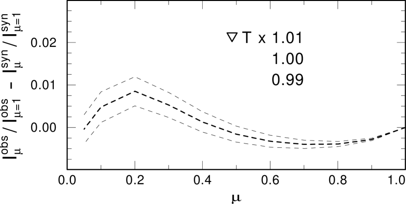
Figure 4: Residual continuum CLV’s at 3499.47 Å from the 1-D model with modified temperature fields. The temperature gradient at $\tau\approx 2/3$ is changed by +1% (upper curve) and -1% (lower curve). The unaltered data are highlighted.

Figure 5: Residual CLV’s in the continuum, i.e. the difference of the observed and the synthetic normalized CLV’s for the 3-D model (solid) and its 1-D approximation (dashed). In comparison, the approximation in 1-D, i.e. the ’horizontal’ time average of the 3-D model, fails to reproduce the observed Center-to-Limb variation at all. The maximum absolute residual is up to 5 times larger, i.e. -0.15 (1-D) vs. 0.03 (3-D).

Finally, we compare the CLV in the continuum for the average (’horizontal’ and over time) 3-D model with the exact data derived from the radiation transfer in 3-D. Fig. 5 shows the residual CLV’s for both models. The discrepancies with the observations are much more severe for the average 3-D model and it becomes obvious that it does not represent the original 3-D time series at all. Although a 1-D representation would obviously be highly desirable because it would allow to quickly calculate spectra by means of a 1-D radiation transfer code, this turns out to be a very poor approximation in this case.

Ayres et al. (2006) have carefully investigated the rotational-vibrational bands of carbon monoxide (CO) in the solar spectrum and have derived oxygen abundances from three models, i.e. the Fal C model (Fontenla et al., 1993), a 1-D model that is especially adapted to match the Center-to-Limb variation of the CO-bands (COmosphere), and from the averaged 3-D time series. In all three cases, temperature fluctuations are accounted for in a so-called 1.5-D approximation, in which profiles from 5 different temperature structures are averaged. By assuming a C/O ratio of 0.5, Ayres et al. (2006) derive a high oxygen abundance close to the “old” value from Grevesse & Sauval (1998) from both the Fal C and the COmosphere model, discarding the low oxygen abundance derived from the mean 3-D model because its temperature gradient is too steep around $\tau_{\rm 0.5\,\mu m}\approx 1$ and fails to reproduce the observed Center-to-Limb variations.

Our current study documents that the mean 3-D model is not a valid approximation of the 3-D time series, and therefore its performance cannot be taken as indicative of the performance of the 3-D model, and in particular of its temperature profile. We find that the Center-to-Limb variation of the continuum predicted by the 3-D simulation matches reasonably well (i.e. similar to the best 1-D model in our study) the observations. The results by Scott et al., based on 3-D radiative transfer on the same hydrodynamical simulations used here, indicate that the observed CO ro-vibrational lines are consistent with the low oxygen and carbon abundances. Our results show that there is no reason to distrust the 3-D-based abundances on the basis of the simulations having a wrong thermal profile.

3.2 Lines

We study the Center-to-Limb variation of a number of lines by comparing observations of the quiet Sun taken at 6 different heliocentric angles to synthetic profiles derived from 3-D and 1-D models. The observations are described in detail by Allende Prieto et al. (2004) and were previously used for the investigation of inelastic collisions with neutral hydrogen on oxygen lines formed under non-LTE conditions. The observations cover 8 spectral regions obtained at 6 different positions on the Sun. The first 5 slit positions are centered at heliocentric angles of $\mu\equiv{\rm cos}\,\theta=$ 1.00, 0.97, 0.87, 0.71 and 0.50. The last position varies between $\mu=$ 0.26 and 0.17 for different wavelength regions. This translates to distances of the slit center from the limb of the Sun in arc min of 16.00’, 12.11’, 8.11’, 4.74’, 2.14’, 0.54’ and 0.24’, assuming a diameter of the Sun of 31.99’. For both of these last positions the slit extends beyond the solar disk and the center of the illuminated slit corresponds to $\mu=$ 0.34 and 0.31 (0.96’ and 0.78’).

We have calculated a variety of line profiles for the 6 positions defined by the center (in $\mu$) of the illuminated slit. Although the slit length, 160 arcsec, is rather large, test calculations show that averaging the spectrum from six discrete $\mu$-angles spanning the slit length gives virtually the same equivalent width than the spectrum from the central $\mu$. For $\mu=0.5$, the second last angle, the difference amounts to a marginal change of the log-$gf$ value of about 0.01. To further reduce the computational burden we have derived the average 3-D profiles from calculations taking only 50 (every other) of the 99 snapshots into account.

We have selected 10 seemingly unblended lines from 5 different neutral ions. The list of lines is compiled in Table 1. The log-$gf$ values for most lines were adopted from laboratory measurements at Oxford (e.g. Blackwell et al. (1995) and references therein) and by O’Brian et al. (1991).

Table 1: Lines

Ion	$\lambda$	$R^{\prime}$	max($\theta$)	log-$gf$	log $\Gamma_{\rm Rad}$	log $\Gamma_{\rm Stark}$	log $\Gamma_{\rm VdW}$
	[Å]		[deg]
Fe I	5242.5	56000	75	-0.970	7.76	-6.33	-7.58
Fe I	5243.8	56000	75	-1.050	8.32	-4.61	-7.22
Fe I	5247.0	56000	75	-4.946	3.89	-6.33	-7.82
Fe I	6170.5	77000	80	-0.380	8.24	-5.59	-7.12
Fe I	6200.3	206000	75	-2.437	8.01	-6.11	-7.59
Fe I	7583.8	176000	80	-1.880	8.01	-6.33	-7.57
Cr I	5247.6	56000	75	-1.627	7.72	-6.12	-7.62
Ni I	5248.4	56000	75	-2.426	7.92	-4.64	-7.76
Si I	6125.0	77000	80	-0.930	$\cdots$	$\cdots$	$\cdots$
Ti I	6126.2	77000	80	-1.425	6.85	-6.35	-7.73

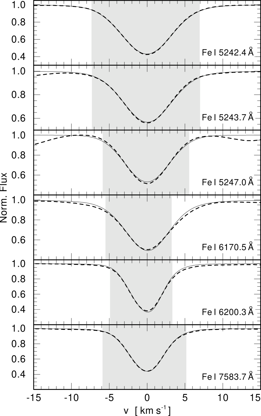
Figure 6: Iron lines under consideration. Observed (dashed) and synthetic (solid) profiles are shown for the disk center. The grey areas mark the velocity ranges used for the calculation of the line equivalent widths. The zero of the velocity scale refers always to the center of the observed line profile, as approximately determined by polynomial fitting. The log-$gf$ values are modified to match the observed line equivalent widths. For most lines the profiles match well. However, the synthetic profile of the line at 5247.0 Å seems to be broader than the observed profile. The line at 6200.3 Å is marginally blended around +5 km s^-1. The line at 6170.5 Å is noticeable blended around +5 km s^-1. For both lines the wavelength interval is decreased accordingly.

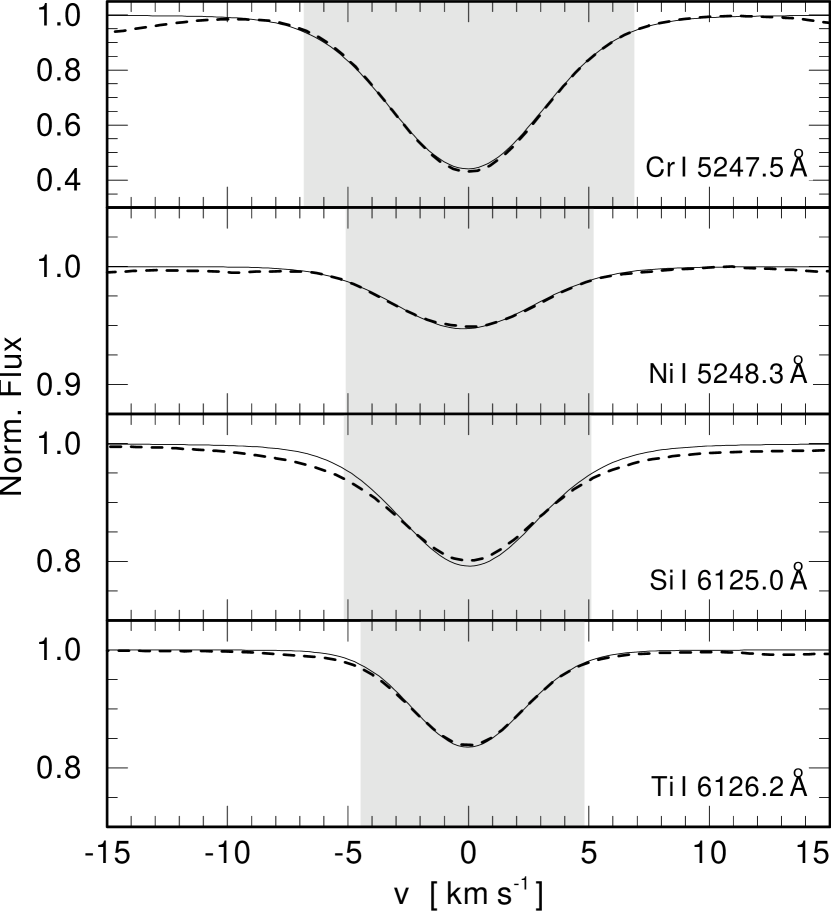
Figure 7: Non-iron lines under consideration. Observed (dashed) and synthetic (solid) profiles are shown for the center disk. The grey areas mark the wavelength ranges used for the calculation of the line equivalent widths. The log-$gf$ values are modified to match the observed line equivalent widths. For most lines the profiles match well. However, the synthetic profile of the Si I line at 6125.0 Å is noticeably narrower than observed.

We are interested in how synthetic lines profiles deviate from observations as a function of the position angle $\mu$ for two reasons. First of all, any clear trend with $\mu$ would reveal shortcomings of the theoretical model atmospheres similar to our findings presented in Sect. 3.1. But, arguably, even more relevant is the fact that any significant deviation (scatter) would add to the error bar attached to a line-based abundance determination.

In our present study we compare synthetic line profiles from 3-D and 1-D models with the observations. Due to the inherent deficiencies of the latter models, i.e. no velocity fields and correspondingly narrow and symmetric line profiles, etc., we focus on line strengths and compare observed and synthetic line equivalent widths, rather than comparing the line profiles in detail. To be able to detect weak deviations, we have devised the following strategy. We have identified wavelength intervals around each line under consideration for the contribution to the line equivalent widths and have calculated series of synthetic line profiles in 1-D and 3-D with varied log-$gf$ values that encircle the observations with respect to their equivalent widths. That allowed us to determine by interpolation the log-$gf$ value required to match the observed line equivalent widths separately for each position angle (“Best-Fit”). To keep interpolation errors at a marginal level we have applied a small step of $\Delta$(log-$gf)=0.05$ for these series of calculations. A simple normalization scheme has been applied. All profiles have been divided by the maximum intensity found in the vicinity of the line center(within $\pm 15\,{\rm km\,s^{-1}}$). We convolved the synthetic profiles with a Gaussian as to mimic the instrumental profile (see Table 1). An additional Gaussian broadening is applied to the line profiles from the 1-D calculation to account for macro-turbulence; this value was adjusted for each line in order to reproduce the line profiles observed at the disk center.

Finally we have translated variations of line strength into variations of abundance, i.e. we have identified $\Delta$ log-($gf$) = $\Delta$log-$\epsilon$. This approximation is valid because the impact of slight changes in a metal abundance on the continuum in the optical is marginal. Note that it is not the intent of this study to derive metal abundances from individual lines. Such an endeavor would require a more careful consideration regarding line blends, continuum normalization, and non-LTE effects.

All calculations described in this section are single-line calculations, i.e. no blends with atomic or molecular lines are accounted for. The observations did not have information on the absolute wavelength scale (see Allende Prieto et al. 2004), but that is not important for our purposes and the velocity scales in Figs. 6 and 7 are relative to center of the line profiles. The individual synthetic profiles were convolved with a Gaussian profile to match the observed profiles (cf. Table 1). We were generally able to achieve a better fit of the observations when slightly less broadening was applied to the 3-D profiles (0.3% in case of Fe I 5242.5). Since we know from previous investigations that the theoretical profiles derived from 3-D Hydro-models match the observations well, we argue that the resolution of the observations is actually slightly higher than estimated by Allende Prieto et al. (2004). An alternative explanation would be that the amplitude of the velocity field in the models is too high. Such a finding, if confirmed, deserves a deeper investigation but is beyond the scope of this study since line equivalent widths are only marginally (if at all) affected.

We introduce the lines under consideration by showing the observed center-disk line profiles and the “Best-Fits” derived from the 3-D calculations of the six Fe I lines and the four lines from other ions in Figs. 6 and 7, respectively. In Fig. 8 we exemplify the fitting process by means of the Fe I line at 5242.5 Å and show the relative difference between the observation and a variety of model calculations for all 6 angles under consideration. The “Best-Fit” log-$gf$ values are derived by interpolation to match the observed equivalent widths from the spectral region around the line profile.

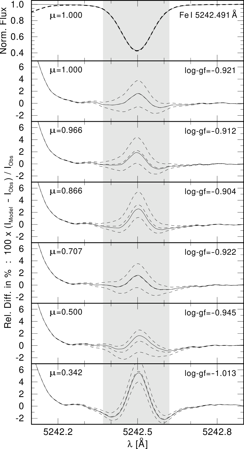
Figure 8: Fit of the Fe I line at 5242.5 Å with synthetic profiles derived from the 3-D Hydro model. Upper panel: Normalized profiles of the center disk observation (dashed) and the “Best-Fit” synthetic profile (solid). Lower panels: Relative difference of the observation and three synthetic profiles (dashed), i.e. three different ${\rm log}\,gf$-values for the 6 angles under consideration. The equivalent widths of the “Best-Fits” (solid) match the observed equivalent widths. The wavelength range considered for the equivalent width is highlighted in grey. The fit improves when a slightly higher resolution (by $\approx 0.3\%$) is assumed. However, line equivalent widths are only marginally affected.

We have obtained “Best-Fits” for all 10 lines (cf. Table 1) and present the log-$gf$ values as a function of $\mu$ in Fig. 9. Be reminded that the aim of this study is not the measurement of absolute abundances: we focus on relative numbers and normalize our results with respect to the disk center ($\mu=1$).

For improved readability we subdivide our findings presented in Fig. 9 into 4 distinct groups, i.e. iron/non-iron lines and 1-D/3-D calculations, respectively. We focus our discussion on the first five data points because we have some indications that the data obtained for the shallowest angle is less trustworthy than the data from the other angles: i) the relative contribution of scattered light was estimated from the comparison of the center-disk spectrum with the FTS spectrum taken from Brault & Neckel (1987), and the outer-most position was the only one for which the entire slit was not illuminated, ii) for all 10 lines the fit of the line profiles for this particular angle is the worst (cf. Fig. 8) and iii) the scatter in our data presented in Fig. 9 is the largest for this angle. Fortunately, the flux integration is naturally biased towards the center of the disk.

We find this systematic behavior for all 6 iron lines: $\Delta{\rm log}(\epsilon)$ is larger or equal in 1-D compared to 3-D, for all but one line (Fe I 6170.5 Å) $\Delta{\rm log}(\epsilon)$ is positive or zero for the 1-D calculations, and $\Delta{\rm log}(\epsilon)$ is negative or zero for all 3-D calculations. The Fe I line at 6170.5 Å stands out in both comparisons. In 1-D it is the only line with a negative $\Delta{\rm log}(\epsilon)$ and in 3-D it shows the by far largest negative $\Delta{\rm log}(\epsilon)$. This might be related to the noticeable line blend (cf. Fig. 6).

The iron lines calculated in 3-D indicate a uniform trend of decreased log-$gf$ values with increased distance from the center-disk. The average decrease at $\mu=0.5$ for this group is -0.015 (Fe I 6170.5 Å excluded). From the 1-D calculations we derive the opposite trend for the same group of lines and obtain an average of 0.103. Obviously, the 3-D model performs significantly better than the 1-D reference model regarding the center-to-limb variation of Fe I lines, even when equivalent widths, and not line asymmetries or shifts, are considered.

For these five Fe I lines we obtain an average difference (1-D vs. 3-D) of 0.12 at $\mu=0.5$. To estimate the impact on abundance determinations based on solar fluxes we apply a 3-point Gaussian integration, neglecting the shallowest angle at $\mu=0.11$ (which has, by far, the smallest integration weight) for which we have no data, and assuming that the good agreement between the 1-D and the 3-D calculations for the central ray implies an equally good agreement for the first angle at $\mu=0.89$. These estimates lead to an abundance correction of approximately 0.06 dex between 1-D and 3-D models due to their different center-to-limb variation. Asplund et al. (2000) found a similar correction from the comparison of 1-D and 3-D line profiles at the disk center.

For the 4 non-iron lines we find a uniform trend of increasing log-$gf$ values with decreasing $\mu$ for both, the 1-D and the 3-D dataset. The systematic behavior is similar to what we find for the iron lines, but now the performance of the 1-D and 3-D models is similar, and the offsets are in the same sense: larger abundances would be found towards the limb for both models.

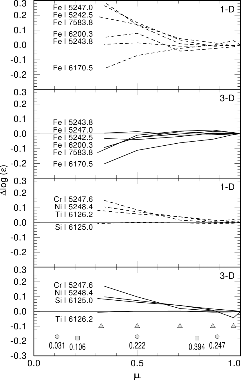
Figure 9: Relative abundance variations with respect to the center disk ($\mu\!\!=\!\!1$) from the 1-D (dashed) and the 3-D calculations, respectively. The upper two panels show the six Fe I lines, the lower two panels show the four lines from the other elements. Line designations are given in the left part of the plot. In the second panel from the top, the curves for the iron lines at 5242.5 and 6200.3 Å overlap with each other for the two positions closest to the limb. The bottom panel also indicates the six $\mu$-angles of the observations (triangles, $\mu\!\!=\!\!1$ not shown, shallowest angles varies slightly) and the $\mu$-angles used in a 2-point (squares) and a 3-point (circles) Gaussian flux integration and their respective integration weights ($\sum$ $w_{\mu}=0.5$).

4 Conclusion

The photosphere of cool stars and the Sun can be described by stellar atmospheres in 1-D and 3-D. Since the 3-D models add more realistic physics, i.e. the hydrodynamic description of the gas, they can be seen truly as an advancement over the 1-D models. However, this refinement increases the computational effort by many orders of magnitude. In fact, the computational workload becomes so demanding, that the description of the radiation field has to be cut back to very few frequencies, i.e. to a rudimentary level that had been surpassed by 1-D models over 30 years ago. Overall we are left with the astonishing situation that a stellar photosphere can be modeled by either an accurate description of the radiation field with the help of a makeshift account of stellar convection (Mixing-length theory), or by an accurate description of the hydrodynamic properties augmented by a rudimentary account of the radiation field.

It is evident that individual line profiles can be described to a much higher degree and without any artificial micro- or macro-turbulence by the 3-D Hydro models, as the simulations account for Doppler-shifts from differential motions within the atmosphere. We know from detailed investigations of line profiles that the velocity field is described quite accurately and that the residuals of the fittings to line profiles are reduced by about a factor of 10. However, it is not obvious how the 3-D models compare to their 1-D counterparts when it comes to reproduce spectral energy distributions and line strengths.

We study the solar Center-to-Limb variation for several lines and continua, to probe the temperature structure of 3-D models. The work is facilitated by the new code Ass$\epsilon$t, which allows for the fast and accurate calculation of spectra from 3-D structures. In comparisons to other programs (e.g. Asplund et al. (2000); Ludwig & Steffen (2007)), the attributes of the new code are a greater versatility, i.e. the ability to handle arbitrarily complicated lines blends on top of non-constant background opacities, higher accuracy due to the proper incorporation of scattering and improved (higher-order) interpolation schemes, and a higher computational speed.

In our study we find that regarding center-to-limb variations, the overall shortcomings of the 3-D model are roughly comparable to the shortcomings of the 1-D models. Firstly, we conclude from the investigation of the continuum layers that the models’ temperature gradient is too steep around $\tau\approx 2/3$. This behavior is more pronounced for the 3-D model which shows a drop in intensity (with $\mu$) that is about twice the size of the drop displayed by our reference 1-D model, but at the same time smaller than the discrepancies found for two other (newer!) 1-D structures. Secondly, the line profiles for different position angles on the Sun cannot be reproduced by a single abundance. For Fe I lines, the abundance variation between the disk center and $\mu=0.5$ is about 0.1 dex for our reference 1-D model, but only $0.015$ dex (and with the opposite sign) for the 3-D simulations, albeit the calculations for lines of other neutral species suggest a more balanced outcome.

Overall we conclude that the 1-D and the 3-D models match the observed temperature structure to a similar degree of accuracy. This is somewhat surprising but it might be that the improved description of the convective energy transport is offset by deficiencies introduced by the poor radiation transfer. Once new Hydro models based on an upgraded radiation transfer scheme (i.e. more frequencies and angles, better frequency binning) become available in the near future (Asplund, priv. comm.), we will be able to test this hypothesis. It will become clear whether focusing on refining the radiation transfer will be enough to achieve better agreement with observations, or the hydrodynamics needs to be improved as well.

References

- Allende Prieto et al. (2001) Allende Prieto, Lambert, D. L., Asplund, M. 2001, ApJ, 556, L63
- Allende Prieto et al. (2002) Allende Prieto, Lambert, D. L., Asplund, M. 2002, ApJ, 567, 544
- Allende Prieto et al. (2003) Allende Prieto, C., Lambert, D. L., Hubeny, I., Lanz, T. 2003, ApJS, 147, 363
- Allende Prieto et al. (2004) Allende Prieto, C., Asplund, M., Bendicho, P. F. 2004, A&A, 423, 1109
- Allende Prieto et al. (2006) Allende Prieto, C., Beers, T. C., Wilhelm, R., Newberg, H. J., Rockosi, C. M., Yanny, B., Lee, Y. S. 2006, ApJ, 636, 804
- Allende Prieto (2007) Allende Prieto, C. 2007, Invited review to appear in the proceedings of the 14th Cambridge Workshop on Cool Stars, Stellar Systems, and the Sun; G. van Belle, ed. (Pasadena, November 2006), astro-ph/0702429
- Asplund et al. (1999) Asplund, M., Nordlund, Å, Trampedach, R., & Stein, R. F. 1999, A&A, 346, L17
- Asplund et al. (2000) Asplund, M., Nordlund, Å, Trampedach, R., Allende Prieto, C., & Stein, R. F. 2000, A&A, 359, 729
- Asplund et al. (2004) Asplund, M., Grevesse, N., Sauval, A. J., Allende Prieto, C., Kiselman, D. 2004, A&A, 417, 751
- Asplund et al. (2005a) Asplund, M., Grevesse, N., & Sauval, A. J. 2005a, Cosmic Abundances as Records of Stellar Evolution and Nucleosynthesis, 336, 25
- Asplund et al. (2005b) Asplund, M., Grevesse, N., Sauval, A. J., Allende Prieto, C., Kiselman, D. 2005b, A&A, 461, 693
- Auer (2003) Auer, L., 2003, Formal Solution: EXPLICIT Answers in Stellar Atmosphere Modeling, ASP Conference proceedings, 2003, Vol. 288, Hubeny I., Mihalas D., Werner K. (eds)
- Ayres et al. (2006) Ayres, T. R., Plymate, C., Keller, C. U. 2006, A&A, 165, 618
- Bahcall et al. (2005) Bahcall, J. N., Basu, S., Pinsonneault, M., & Serenelli, A. M. 2005, ApJ, 618, 1049
- Barklem et al. (2000) Barklem, P. S., Piskunov, N., O’Mara, B. J. 2000, A&AS, 142, 467
- Bautista (1997) Bautista, M. A. 1997, A&AS, 122, 167
- Blackwell et al. (1995) Blackwell, D. E., Lynas-Gray, A. E., & Smith, G. 1995, A&A, 296, 217
- Brault & Neckel (1987) Brault, J., & Neckel, H. 1987, Spectral Atlas of Solar Absolute Disk-Averaged and Disk-Center Intensity from 3290 to 12150 Å, unpublished, Tape copy from KIS IDL library
- Delahaye & Pinsonneault (2006) Delahaye, F., & Pinsonneault, M. H. 2006, ApJ, 649, 529
- Elste & Gilliam (2007) Elste, G., Gilliam, L. 2007, Sol. Phys., 240, 9
- Fontenla et al. (1993) Fontenla, J. M., Avrett, E. H., Loeser, R. 1993, ApJ, 406, 319
- Grevesse & Sauval (1998) Grevesse, N., & Sauval, A. J. 1998, in: Frölich C., Huber M.C.E., Solanki S.K., von Steiger R. (eds), Solar composition and its evolution — from core to corona, Dordrecht: Kluwer, p. 161
- Gray (1992) Gray, D. F. 1992, The Observation and Analysis of Stellar Photospheres, 2nd edition, Cambridge Universiy Press, Cambridge
-
Hubeny & Lanz (1995)
Hubeny, I., Lanz, T. 1995
“SYNSPEC — A Users’s Guide”
http://nova.astro.umd.edu/
Tlusty2002/pdf/syn43guide.pdf - Koesterke et al. (in prep.) Koesterke, L., Allende Prieto, C., Lambert, D. L. 2006, submitted to ApJ
- Koesterke et al. (in prep.) Koesterke, L., Allende Prieto, C., Lambert, D. L. 2006, in prep. for ApJ
- Kurucz et al. (1984) Kurucz, R. L., Furenlid, I., Brault, J., & Testerman, L. 1984, National Solar Observatory Atlas, Sunspot, New Mexico: National Solar Observatory, 1984,
- Kurucz (1993) Kurucz, R. 1993, ATLAS9 Stellar Atmosphere Programs and 2 km/s grid. Kurucz CD-ROM No. 13. Cambridge, Mass.: Smithsonian Astrophysical Observatory, 1993., 13,
- Lin et al. (2007) Lin, C.-H., Antia, H. M., & Basu, S. 2007, ApJ, in press (ArXiv e-prints, 706, arXiv:0706.3046)
- Ludwig & Steffen (2007) Ludwig, H.-G., Steffen, M. 2007, arXiv:0704.1176
- Nahar (1995) Nahar, S. N. 1995, A&A, 293, 967
- Neckel (2003) Neckel, H. 2003, Sol. Phys., 212, 239
- Neckel (2005) Neckel, H. 2005, Sol. Phys., 229, 13