Goos-Hänchen-Like Shifts in Atom Optics

Abstract

We consider the propagation of a matter wavepacket of two-level atoms through a square potential created by a super-Gaussian laser beam.  We explore the matter wave analog of Goos-Hänchen shift within the framework of atom optics where the roles of atom and light is exchanged with respect to conventional optics.  Using a vector theory, where atoms are treated as particles possessing two internal spin components, we show that not only large negative but also large positive Goos-Hänchen shifts can occur in the reflected atomic beam.

I Introduction

In conventional optics for light waves, Goos-Hänchen in 1947 discovered that a light beam under the condition of total reflection can experience a lateral shift (or displacement) along the surface of a dielectric boundary Goos .    This pioneering work has stimulated a large volume of studies Artmann ; Chiao ; Li ; WangLG:3 ; Xiang ; Zeng ; Renard ; Tamir ; Wild ; Schlesser ; Pfleghaar ; Lai:2 ; Bonnet ; Lai:1 ; Berman ; Broe ; Kong ; Fan ; Declercq ; Lakhtakia ; Shadrivov ; Felbacq ; Qing ; Chen ; WangLG:1 ; WangLG:2 ; Shen ; Liu:2 ; He ; Tsakmakidis ; Yan  , concerning the Goos-Hänchen shift of reflected or transmitted Chiao ; Li ; WangLG:3 light beams of different polarizations Lai:2 in different media characterized with, for example, periodic structures Bonnet ; Declercq ; Felbacq ; He , (left or right) handedness Shadrivov ; Qing ; Chen ; WangLG:2 , multilayers Tamir , weakly absorbing Lai:1 ; Shen , lower-index Fan or negative-index of refraction Berman , etc.  The key physics behind the Goos-Hänchen shift is the nature of wave interference.  From the perspective of wave optics, the incident beam of a finite transverse width can be viewed as composed of plane wave components, each of which has a slightly different transverse wavevector.  Each wave component, after the total internal reflection, undergoes a different phase shift, and the superposition of all the reflected wave components gives rise to the lateral shift of the intensity peak in the reflected beam Artmann .

In this sense, it is not so much the total internal reflection but rather the phase modulations for different plane wave components that remains the true mechanism behind the lateral shift.  Thus, the Goos-Hänchen shift is expected to occur in matter waves where particles have finite masses.  As is known, under the usual conditions (or temperatures), electrons possess a de Broglie’s wavelength much longer than atoms because the latter is much heavier in mass than the former.  Thus, it is much easier to demonstrate the Goos-Hänchen shift with electrons Miller ; Fradkin or even neutrons Maaza ; Ignatovich than with atoms. The situation, however, has been rapidly changed over the last two decades. Nowadays, ultracold atoms with a relatively long de Broglie’s wavelength can be routinely made available, thanks to the rapid advancement of the laser cooling and trapping technology.  Motivated by the fact that ultracold atoms have led to many important applications in atom optics Meystre , we explore, in this paper, the matter wave analog of Goos-Hänchen effect within the framework of atom optics where matter waves of ultracold atoms are manipulated by laser fields.   An important difference between the matter waves in atom optics and the light waves in conventional optics is that atoms have internal electronic structures while photons are structureless.  Thus, an accurate description of the Goos-Hänchen effect in atom optics must regard atoms as particles possessing internal spins (energy states).  To the best of our knowledge, our work here represents the first that is seriously devoted to the problem of Goos-Hänchen effect with cold atoms.  As such, we limit our goals to establishing a general theoretical framework and to applying it for a basic understanding of the Goos-Hänchen effect in matter waves with cold two-level atoms, while at the same time hoping that our work can draw significant attentions from experimentalists for future applications.

Our paper is organized as follows.  In Sec. II, we derive a set of coupled 1-D Schrödinger equations to describe the scattering of two-level atoms by a super-Gaussian laser beam in a 2-D setting.  In the same section, we present the connection between the lateral shifts and the coefficients of reflection and transmission.  In Sec.  III, we derive, with the help of a dressed state picture, a set of analytical expressions for the reflection and transmission coefficients, which are to be used in Sec. IV to significantly simplify our calculations.  In Sec. IV, we combine the tools developed in Sec. II with those in Sec. III to numerically investigate, within the context of atom optics, the matter wave analog of Goos-Hänchen-like shifts.  Finally, a conclusion will be given in Sec. V.

II Model and Basic Equations

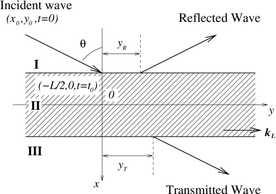
Figure 1: A wave packet of atoms with two internal states impinges on a laser “slab”.

Figure 1 is the schematic of our model, in which a matter wavepacket composed of two-level atoms of transition frequency $\omega_{a}$ is obliquely incident upon a “slab”  made up of a travelling laser beam of frequency $\omega_{L}$ and wavenumber $k_{L}$. In our model, we require that both the atom and laser beams be sufficiently wide along the direction normal to the plane of incidence ($x-y$ plane) so that the degree of freedom in the $z$-dimension can be completely liberated.  Under such a circumstance, we can adopt the following coupled $2-D$ Schrödinger equations Zhang

$$i\dot{\Psi}_{1} =-\frac{\hbar\nabla^{2}}{2m}\Psi_{1}-\frac{\Omega\left(x\right)}{2}e^{-ik_{L}y}\Psi_{2},$$ (1a)

$$i\dot{\Psi}_{2} =\left(-\frac{\hbar\nabla^{2}}{2m}-\Delta-i\frac{\gamma}{2}\right)\Psi_{2}-\frac{\Omega\left(x\right)}{2}e^{ik_{L}y}\Psi_{1},$$ (1b)

to describe the evolution of the wavefunctions, $\Psi_{1}$ and $\Psi_{2}$, of the ground state $\left|1\right\rangle$ and the excited state $\left|2\right\rangle$.  In Eqs. (1), we have defined $m$ as the atomic mass, $\nabla^{2}\equiv\partial^{2}/\partial x^{2}+\partial^{2}/\partial y^{2}$ as the 2-D Laplacian operator, $\Delta=\omega_{L}-\omega_{a}$ as the laser detuning, and $\gamma$ as the decay rate of the excited atomic state.  In addition, we describe the dipole interaction between the laser field and atoms by a Rabi frequency in the form of

$$\Omega\left(x\right)=\Omega F\left(x\right),$$ (2)

where $\Omega$ is the peak value and $F(x)$ is a normalized spatial function, representing the laser profile.  In this paper, the laser is assumed to possess a beam profile in the form of a high-order Gaussian function, $F\left(x\right)=\exp\left[-\left(x^{2}/w_{L}^{2}\right)^{N}\right]$; such a beam is experimentally accessible through spatial shaping techniques Liu:1 ; Belanger ; Dong or optical techniques Zhao .  To further simplify the problem, we restrict our study to the super-Gaussian beam with an order number $N$ so large that, to a fairly good approximation, $F\left(x\right)$ can be idealized as a step function

$$F\left(x\right)=\begin{cases}1,&-L/2<x<L/2,\\ 0,&x>L/2,x<-L/2,\end{cases}$$ (3)

Next, we utilize the fact of the Rabi frequency [Eq. (2)] being $y$ independent to eliminate $y$ in favor of $y$-wavevector $k_{y}$ through the Fourier transformation

$$\Psi_{1}\left(\mathbf{r},t\right) =\int dk_{y}\phi_{1}\left(x,k_{y},t\right)e^{ik_{y}y-\frac{i\hbar k_{y}^{2}}{2m}t},$$ (4a)

$$\Psi_{2}\left(\mathbf{r},t\right) =\int dk_{y}\phi_{2}\left(x,k_{y},t\right)e^{i(k_{y}+k_{L})y-\frac{i\hbar k_{y}^{2}}{2m}t},$$ (4b)

where $\mathbf{r=}\left(x,y\right)$.  By doing so, we transform Eqs. (1) into coupled 1-D Schrödinger equations

$$i\hbar\mathbf{\dot{\phi}=}\left(-\frac{\hbar^{2}}{2m}\frac{\partial^{2}}{\partial x^{2}}\hat{I}+\hat{V}\right)\mathbf{\phi,}$$ (5)

where $\mathbf{\phi}=\left(\phi_{1},\phi_{2}\right)^{T}$ is a two-component vector field, $\hat{I}\,\$is a $2\times 2$ unit matrix, and $\hat{V}$ is the potential matrix given by

$$\hat{V}=-\frac{\hbar}{2}\left[\begin{array}[c]{cc}0&\Omega\\ \Omega&2\left(\delta+\frac{1}{2}i\gamma\right)\end{array}\right].$$ (6)

In Eq. (6), we have defined

$$\delta=\Delta-\frac{\hbar k_{y}k_{L}}{m}-\frac{\hbar k_{L}^{2}}{2m},$$ (7)

as the effective detuning, where $\hbar k_{y}k_{L}/m$ and $\hbar k_{L}^{2}/2m$ are, respectively, the Doppler and the photon recoil frequency.  Equation (5) serves as the starting point for next section, where we calculate the scattering matrix, which determines all the scattering properties of our model.

For now, we turn our attention to the lateral shifts of the reflected and transmitted wavepackets.  For this purpose,  let’s first jump ahead to Eqs. (15) of Sec. III, which define various transmission and reflection coefficients via the stationary scattering solutions in free space.  Of relevance to our interest here are the coefficients of transmission $T_{1}$ and reflection $R_{1}$ of the ground state; we ignore $T_{2}$ and$\ R_{2}$ of the excited state since the excited wave, being highly susceptible to the decay by the spontaneous emission, cannot propagate far from the scattering region.  Let $\Theta_{1}^{R,T}\left(\mathbf{k}\right)$ be the phases of reflection and transmission coefficients defined through the relation

$$S_{1}\left(\mathbf{k}\right)=\left|S_{1}\left(\mathbf{k}\right)\right|e^{i\Theta_{1}^{S}\left(\mathbf{k}\right)},$$ (8)

where for notational simplicity, we have used (and will continue to use) $S=R$ and $S=T$ to symbolize reflection and transmission, respectively.  For an incident wave packet initially ($t=0$) located at $\left(x_{0}\text{, }y_{0}\right)$ far away from the laser beam (see Fig. 1), we can construct, through the superposition of the time-independent solutions [Eqs. (15)], its reflected and transmitted wavepackets in the form of

$$\Psi_{1}^{S}\left(\mathbf{r},t\right)=\int d^{2}\mathbf{k}^{\prime}f\left(\mathbf{k}^{\prime}-\mathbf{k}\right)|S_{1}\left(\mathbf{k}^{\prime}\right)|e^{i\eta_{1}^{S}\left(\mathbf{k}^{\prime},\mathbf{r}\right)}$$ (9)

where $\eta_{1}^{R,T}$ are the total phases defined as

$$\eta_{1}^{R}\left(\mathbf{k}^{\prime},\mathbf{r}\right) =\Theta_{1}^{R}\left(\mathbf{k}^{\prime}\right)-k_{x}^{\prime}\Delta x^{R}+k_{y}^{\prime}\Delta y^{R}-\frac{\hbar{k}^{\prime{2}}t}{2m},$$ (10a)

$$\eta_{1}^{T}\left(\mathbf{k}^{\prime},\mathbf{r}\right) =\Theta_{1}^{T}\left(\mathbf{k}^{\prime}\right)+k_{x}^{\prime}\Delta x^{T}+k_{y}^{\prime}\Delta y^{T}-\frac{\hbar{k}^{\prime}{}^{2}t}{2m},$$ (10b)

with$\ \Delta x^{R}=x+x_{0}$, $\Delta x^{T}=x-x_{0}$, $\Delta y^{R}=\Delta y^{T}=y-y_{0}$, and $k^{\prime 2}={k}^{\prime}{{}_{x}}^{2}+{k}^{\prime}{{}_{y}}^{2}$.  In Eqs. (9), $f\left(\mathbf{k}^{\prime}-\mathbf{k}\right)$ is a (real) weighting function peaked around $\mathbf{k}^{\prime}=\mathbf{k}$ with a momentum distribution sufficiently narrow and smooth that Eqs. (9) represent fairly accurately the plane waves of velocity $\hbar\mathbf{k}/m$.  Equation (9) indicates that the reflected and transmitted waves are the result of interference among different wave components distinguished by wavevector $\mathbf{k}^{\prime}=\left(k_{x}^{\prime},k_{y}^{\prime}\right)$.  As a result, the values of these waves at a given time and location, $\left(\mathbf{r},t\right)$, depend crucially on the phases [Eqs. (10)] of each $\mathbf{k}^{\prime}$ component.  In particular, $\Psi_{1}^{R,T}\left(\mathbf{r},t\right)$ reach peak values when a constructive interference takes place or equivalently when $\nabla_{\mathbf{k}^{\prime}}\eta_{1}^{R,T}$ at $\mathbf{k}^{\prime}=\mathbf{k}$ vanish.   Using this condition, we find that the peaks of the wavepackets in the coordinate space propagate with time according to

$$\Delta x^{R} =-\frac{\hbar k_{x}}{m}t+\frac{\partial\Theta_{1}^{R}}{\partial k_{x}},\ \Delta y^{R}=\frac{\hbar k_{y}}{m}t-\frac{\partial\Theta_{1}^{R}}{\partial k_{y}},$$ (11a)

$$\Delta x^{T} =+\frac{\hbar k_{x}}{m}t-\frac{\partial\Theta_{1}^{T}}{\partial k_{x}},\ \Delta y^{T}=\frac{\hbar k_{y}}{m}t-\frac{\partial\Theta_{1}^{T}}{\partial k_{y}},$$ (11b)

where all the derivatives are assumed to be taken at $\mathbf{k}^{\prime}=\mathbf{k}$.

Let $t_{0},$ $t_{R}$ and $t_{T}$ be, respectively, the time duration of the atomic beam between $t=0$ and right before it hits the boundary at $x=-L/2$, between $t=0$ and immediately after it is reflected from the boundary at $x=-L/2$, and between $t=0$ and right after it is transmitted from the boundary at $x=L/2$.  In terms of $t_{0}$, we have $x_{0}=-(L/2+\hbar k_{x}t_{0}/m)$ and $y_{0}=-\hbar k_{y}t_{0}/m$, which, when substituted into Eqs. (11) for $\Delta x^{R,T}$, allows us to find $t_{R,T}$

$$\Delta t_{S}=t_{S}-t_{0}=\frac{m}{\hbar k_{x}}\left(\frac{\partial\Theta_{1}^{S}}{\partial k_{x}}+L\right).$$ (12)

Finally, by incorporating these results into Eqs. (11) for $\Delta y^{R,T}$, we find that the induced Goos-Hänchen-like lateral shift $y_{R}$ due to the reflection and $y_{T}$ due to the transmission (see Fig. 1) are governed by

$$y_{S}=\frac{\hbar k_{y}}{m}\Delta t_{S}-\frac{\partial\Theta_{1}^{S}}{\partial k_{y}}.$$ (13)

where $\ \partial\Theta_{1}^{S}/\partial k_{i}$ ($i=x,y$ and $S=R,T$) are evaluated using

$$\frac{\partial\Theta_{1}^{S}}{\partial{k_{i}}}=-i\left[\frac{1}{S_{1}}\frac{\partial S_{1}}{\partial{k_{i}}}-\frac{1}{\left|S_{1}\right|}\frac{\partial\left|S_{1}\right|}{\partial{k_{i}}}\right],$$ (14)

which is a direct consequence of Eq. (8).  In contrast to the usual shifts, which are solely determined by the part directly proportional to $\Delta t_{S}$, the lateral shifts in Eq. (13) contain an additional term $\partial\Theta_{1}^{S}$/$\partial k_{y}$.  This is a unique aspect of atom optics, where momentum conservation during the photon emission and absorption makes the effective laser detuning $\delta$ [Eq. (7)] $k_{y}$ dependent.   As a result, the phase $\Theta_{1}^{S}$ becomes a function of $k_{y}$ via its dependence on $\delta$, which, in turn, leads to a finite $\partial\Theta_{1}^{S}$/$\partial k_{y}$.

From this derivation, it is clear that (a) the Goos-Hänchen-like lateral shifts are the wave phenomena, that depend crucially on the ability of the optical potential to modify the phases of various matter wave components, and (b) the key to the lateral shifts is the transmission and reflection coefficients, which will be the focus of our study in the next section.

III Transmission and Reflection Coefficients

In this section, we construct the reflection and transmission coefficients, starting from the stationary scattering solutions of Eq. (5) for an incident ground atomic beam having an energy $E_{x}=\hbar k_{x}^{2}/2m$ and wavenumber $k_{x}$ along the $x$ dimension.  Let’s first introduce the reflection and transmission coefficients for the ground state, $R_{1}$ and $T_{1}$, and those for the excited state, $R_{2}$ and $T_{2}$, via the scattering solutions in regions I and III.  By virtue of the decoupling between the excited and ground states in free propagation regions I and III outside the laser slab, the scattering solutions take the form

$$\mathbf{\phi}^{I} =\left(\begin{array}[c]{c}e^{ik_{1}x}+R_{1}e^{-ik_{1}x}\\ R_{2}e^{-ik_{2}x}\end{array}\right)e^{-i\frac{E_{x}}{\hbar}t},$$ (15c)

$$\mathbf{\phi}^{III} =\left(\begin{array}[c]{c}T_{1}e^{ik_{1}x}\\ T_{2}e^{ik_{2}x}\end{array}\right)e^{-i\frac{E_{x}}{\hbar}t},$$ (15f)

where we have defined the free-space wavevectors

$$k_{1}=k_{x},k_{2}=\sqrt{2\frac{m}{\hbar}\left(\delta+i\frac{\gamma}{2}\right)+k_{x}^{2}}.$$ (16)

The excited-state and ground-state components in region II are, however, mixed because Eq. (5) is a coupled equation. To solve Eq. (5) and thus, to find the vector wavefunction $\mathbf{\phi}^{II}$ in region II, we first seek to diagonalize the matrix $\hat{V}$ [Eq. (6)] by looking for the eigenvectors of $\hat{V}$.   This leads to two eigenvalues $V_{+}$ and $V_{-}$, given by

$$V_{\pm}=\frac{\hbar}{2}\left[-\left(\delta+i\frac{\gamma}{2}\right)\pm\sqrt{\left(\delta+i\frac{\gamma}{2}\right)^{2}+\Omega^{2}}\right].$$ (17)

The corresponding eigenvectors are expressed as the first and second column vectors of the following transformation matrix

$$U=\left(\begin{array}[c]{cc}\sin\varphi&\cos\varphi\\ -e^{i\beta}\cos\varphi&e^{-i\beta}\sin\varphi\end{array}\right),$$ (18)

where $\varphi$ and $\beta$, defined as

$$\tan\varphi=\frac{\hbar\Omega}{2\left|V_{+}\right|},V_{+}=\left|V_{+}\right|e^{i\beta},$$ (19)

are two angles introduced to characterize the dressed states

$$\left|+\right\rangle =\sin\varphi\left|1\right\rangle-e^{i\beta}\cos\varphi\left|2\right\rangle,$$ (20a)

$$\left|-\right\rangle =\cos\varphi\left|1\right\rangle+e^{-i\beta}\sin\varphi\left|2\right\rangle,$$ (20b)

The inverse of $U$, which will also be an important part of the scattering problem involving vector matter waves, is given by

$$U^{-1}=f\left(\begin{array}[c]{cc}e^{-i\beta}\sin\varphi&-\cos\varphi\\ e^{i\beta}\cos\varphi&\sin\varphi\end{array}\right)$$ (21)

where $f=\left(e^{-i\beta}\sin^{2}\varphi+e^{i\beta}\cos^{2}\varphi\right)^{-1}$ is a normalization factor.  In the absence of spontaneous decay $\gamma=0$, we have $\beta=0$, and $U$ becomes unitary. The dressed states can be simplified into the ones well-known in quantum optics Jaynes .  The presence of the spontaneous decay renders the Hamiltonian nonhermitian Delgado , which is why $U$ is no longer a unitary matrix when $\beta$ $\neq 0$ as one can easily verify from Eq. (18).

With these preparations, we now express $\mathbf{\phi}^{II}$, in terms of wavefunctions $\phi_{\pm}$ on the dressed-state basis, as

$$\mathbf{\phi}^{II} =U\left(\begin{array}[c]{c}\phi_{+}\\ \phi_{-}\end{array}\right)e^{-i\frac{E_{x}}{\hbar}t},$$ (24)

$$\equiv U\left(\begin{array}[c]{c}A_{1}e^{\alpha_{1}x}+B_{1}e^{-\alpha_{1}x}\\ A_{2}e^{\alpha_{2}x}+B_{2}e^{-\alpha_{2}x}\end{array}\right)e^{-i\frac{E_{x}}{\hbar}t},$$ (27)

where $A_{i}$ and $B_{i}$ are the superposition coefficients, and for easy organization, we introduce $\alpha_{1}\equiv\alpha_{+}$ and $\alpha_{2}\equiv\alpha_{-}$, where

$$\alpha_{\pm}=\sqrt{2mV_{\pm}/\hbar^{2}-k_{x}^{2}}.$$ (28)

To facilitate the derivation bellow, besides $U$  and $U^{-1}$, we also introduce the matrix $W$ and its inverse $W^{-1},$ where

$$W=\left(\begin{array}[c]{cc}ik_{1}&0\\ 0&ik_{2}\end{array}\right)^{-1}U,W^{-1}=U^{-1}\left(\begin{array}[c]{cc}ik_{1}&0\\ 0&ik_{2}\end{array}\right)$$ (29)

or equivalently,

$$W_{ij}=\left(ik_{i}\right)^{-1}U_{ij},\left(W^{-1}\right)_{ij}=ik_{j}\left(U^{-1}\right)_{ij}\text{. \ }$$ (30)

Next, we require that $\phi^{I,II,III}$ and their derivatives be continuous at location $x=L/2,$ leading to

$$\left(\begin{array}[c]{c}u_{1}\\ u_{2}\end{array}\right) =U^{-1}\left(\begin{array}[c]{c}T_{1}e^{ik_{1}L/2}\\ T_{2}e^{ik_{2}L/2}\end{array}\right),$$ (31e)

$$\left(\begin{array}[c]{c}v_{1}\\ v_{2}\end{array}\right) =W^{-1}\left(\begin{array}[c]{c}T_{1}e^{ik_{1}L/2}\\ T_{2}e^{ik_{2}L/2}\end{array}\right)$$ (31j)

where $\left(u_{i},v_{i}\right)$ are a set of new variables defined as

$$u_{i} =A_{i}e^{\alpha_{i}\frac{L}{2}}+B_{i}e^{-\alpha_{i}\frac{L}{2}},$$ (32a)

$$v_{i} =\alpha_{i}\left(A_{i}e^{\alpha_{i}\frac{L}{2}}-B_{i}e^{-\alpha_{i}\frac{L}{2}}\right)$$ (32b)

Similarly, application of the continuation conditions at location $x=-L/2$ results in

$$U\left(\begin{array}[c]{c}x_{1}\\ x_{2}\end{array}\right) =\left(\begin{array}[c]{c}e^{-ik_{1}L/2}+R_{1}e^{ik_{1}L/2}\\ R_{2}e^{ik_{2}L/2}\end{array}\right),$$ (33e)

$$W\left(\begin{array}[c]{c}y_{1}\\ y_{2}\end{array}\right) =\left(\begin{array}[c]{c}e^{-ik_{1}L/2}-R_{1}e^{ik_{1}L/2}\\ -R_{2}e^{ik_{2}L/2}\end{array}\right),$$ (33j)

where $\left(x_{i}\text{,}y_{i}\right)$ are defined in terms of $\left(A_{i},B_{i}\right)$ as

$$\begin{split}x_{i}&=A_{i}e^{-\alpha_{i}\frac{L}{2}}+B_{i}e^{\alpha_{i}\frac{L}{2}},\\ y_{i}&=\alpha_{i}\left(A_{i}e^{-\alpha_{i}\frac{L}{2}}-B_{i}e^{\alpha_{i}\frac{L}{2}}\right).\end{split}$$ (34)

By combining all these conditions (for details see the Appendix), we arrive at a set of compact formulas for the transmission coefficients

$$T_{1} =\frac{2M_{22}^{\left(+\right)}}{M_{11}^{\left(+\right)}M_{22}^{\left(+\right)}-M_{12}^{\left(+\right)}M_{21}^{\left(+\right)}}e^{-ik_{1}L},$$ (35a)

$$T_{2} =-\frac{2M_{21}^{\left(+\right)}}{M_{11}^{\left(+\right)}M_{22}^{\left(+\right)}-M_{12}^{\left(+\right)}M_{21}^{\left(+\right)}}e^{-i\left(k_{1}+k_{2}\right)L/2},$$ (35b)

and for the reflection coefficients

$$R_{1} =\frac{M_{11}^{\left(-\right)}M_{22}^{\left(+\right)}-M_{12}^{\left(-\right)}M_{21}^{\left(+\right)}}{M_{11}^{\left(+\right)}M_{22}^{\left(+\right)}-M_{12}^{\left(+\right)}M_{21}^{\left(+\right)}}e^{-ik_{1}L},$$ (36a)

$$R_{2} =\frac{M_{21}^{\left(-\right)}M_{22}^{\left(+\right)}-M_{22}^{\left(-\right)}M_{21}^{\left(+\right)}}{M_{11}^{\left(+\right)}M_{22}^{\left(+\right)}-M_{12}^{\left(+\right)}M_{21}^{\left(+\right)}}e^{-i\left(k_{1}+k_{2}\right)L/2},$$ (36b)

where

$$\begin{split}M_{ij}^{\left(\pm\right)}&=\sum_{n=1,2}U_{in}\left(U^{-1}\right)_{nj}\left[{\LARGE~{}}\left(1\pm\frac{k_{j}}{k_{i}}\right)\times~{}\right.\\ &\left.\cosh\left(\alpha_{n}L\right)-i\frac{k_{i}k_{j}\mp\alpha_{n}^{2}}{k_{i}\alpha_{n}}\sinh\left(\alpha_{n}L\right)\right].\end{split}$$ (37)

In the next section, Eqs. (35a) and (36a) will be used in connection with the results from Sec. II to numerically determine the lateral shifts.

IV  Discussion

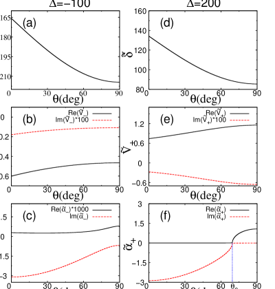
Figure 2: (Color online). The left column calculated under $\tilde{\Delta}=-100$ contains (a) $\tilde{\delta}$, (b) $\tilde{V}_{-}$ , and (c) $\tilde{\alpha}_{-}$ as functions of $\theta$.  The right column calculated under $\tilde{\Delta}=200$ contains (d) $\tilde{\delta}$, (e) $\tilde{V}_{+}$ , and (f) $\tilde{\alpha}_{+}$ as functions of $\theta$.  Other parameters are $\tilde{\gamma}=1,\tilde{k}$ $=3,$ $\tilde{L}=6,~{}\tilde{\Omega}=20$, and $\tilde{k}_{L}=8.1125$.

In this section, we carry out a numerical study of the lateral shifts by first obtaining $\partial\Theta_{1}^{S}/\partial k_{i}$ from Eq. (8) with the help of Eqs. (35a) and (36a), and then determining the lateral shifts using Eqs. (12) and (13).  In our calculation, we replace $k_{x}=k\cos\theta$ and $k_{y}=k\sin\theta$, and correspondingly, $\partial/\partial k_{x}=\cos\theta\partial/\partial k-k^{-1}\sin\theta\partial/\partial\theta$ and $\partial/\partial k_{y}=\sin\theta\partial/\partial k+k^{-1}\cos\theta\partial/\partial\theta$, where $k$ is the magnitude of wavevector and $\theta$ is the incident angle of the atomic wave.  In addition, we adopt the following scaled variables: $\tilde{\Delta}=\Delta/\gamma,\tilde{\Omega}=\Omega/\gamma,$ $\tilde{k}_{L}=k_{L}/k_{\gamma}$, $\hat{k}=k/k_{\gamma}$, $\tilde{L}=L/k_{\gamma}^{-1}$, $\tilde{V}_{\pm}=V_{\pm}/\hbar\gamma$, $\tilde{\alpha}_{\pm}=\alpha_{\pm}/k_{\gamma}$, and $\tilde{y}_{S}=y_{S}/k_{\gamma}^{-1}$, where $k_{\gamma}\equiv\sqrt{2m\gamma/\hbar}$.  In all the examples given bellow, unless stated otherwise, $\tilde{\gamma}=1,\tilde{k}$ $=3,$ $\tilde{L}=6,~{}\tilde{\Omega}=20$, and $\tilde{k}_{L}=8.1125$.

Let’s first consider a case where the laser detuning is set at $\tilde{\Delta}=-100$.  At this $\tilde{\Delta}$, the effective laser detuning $\delta$ remains (deeply) red detuned across all the incident angles as shown in Fig. 2(a).  Under such a circumstance, we have $\left|V_{+}\right|>>$ $\left|V_{-}\right|$ according to Eq. (17) and $\varphi$ approaches a small value according to Eq. (19).  As a result, the scattering properties in this case are largely determined by the $\left|-\right\rangle$ dressed state.  For this reason, we only display in Fig. 2(b) potential $V_{-}$ as “seen” by the atoms in state $\left|-\right\rangle$, which corresponds to a potential well since $Re(V_{-})$ remains negative.  As a result, the $\left|-\right\rangle$ mode function oscillates in the $x$ dimension with a spatial frequency of $Im\left(\alpha_{-}\right)$, whose value is shown in Fig. 2(c)].

Figure 3: The left column contains (a) $\left|R_{1}\right|^{2}$, (b) $\Theta_{1}^{R}$, and (c) $\tilde{y}_{R}$ as functions of $\theta$.  The right column contains (d) $\left|T_{1}\right|^{2}$, (e) $\Theta_{1}^{T}$, and (c) $\tilde{y}_{T}$ as functions of $\theta$ under the condition that $\tilde{\Delta}=-100$ and the rest parameters are the same as in Fig. 2.

The corresponding intensity $\left|S_{1}\right|^{2}$, phase $\Theta_{1}^{S}$, and lateral shift $y_{S}$ of the reflected ($S=R$, left column) and transmitted ($S=T$, right column) waves are displayed in Fig. 3 as functions of the incident angle $\theta$. As our discussion above suggests, we expect to see the phenomenon of resonance scattering by potential wells.  Indeed, in the region where the phase experiences a $\pi$ shift [Fig. 3(b)], the reflectivity $\left|R\right|^{2}$[Fig. 3(a)] approaches a small value while the transmissivity $\left|T\right|^{2}$ [Fig. 3(d)] becomes nearly perfect, which explains the oscillatory behavior exhibited both in $\left|R\right|^{2}$ and in $\left|T\right|^{2}$.  It needs to be stressed that the phase of the reflected wave, as shown in Fig. 3(b), increases (or decreases) sharply, as $\theta$ (or $k_{x}$) sweeps across each resonance.  This causes the reflected wave to experience a large negative Goos-Hänchen shift around each resonance as indicated in Fig. 3(c).

Next, we consider a situation where $\tilde{\Delta}=200$.  With this $\tilde{\Delta}$, $\delta$ remains (deeply) blue detuned for all the incident angles as Fig. 2(d) illustrates.  As a result, according to Eqs. (17) and (19), $\left|V_{+}\right|<<\left|V_{-}\right|$ and $\varphi$ approaches $\pi/2$; the scattering behavior is dominated by the $\left|+\right\rangle$ dressed state.   Here, the laser beam, as illustrated in Fig. 2(e), creates an effective repulsive potential $Re\left(V_{+}\right)>0$. Under such a circumstance and provided that $\hbar^{2}k^{2}/2m>Re\left(V_{+}\right)$, we can introduce a critical angle defined as $\theta_{c}\equiv\cos^{-1}\sqrt{2mRe\left(V_{+}\right)/\hbar^{2}k^{2}}$ at which the ($x$) kinetic energy of the atomic beam equals the height of the potential barrier. (Such a critical angle does not exist for the case of red detuning.)   In our case here, we identify from Fig. 2(f) that $\theta_{c}\approx 69.4^{\circ}$, which has the physical meaning that bellow $\theta_{c}$, the $\left|+\right\rangle$ mode oscillates at a spatial frequency close to $Im\left(\alpha_{+}\right)$ while beyond $\theta_{c}$, it undergoes quantum tunneling with $1/Re\left(\alpha_{+}\right)$ being the characteristic tunneling distance.

Indeed, Fig. 4 shows that $\left|S_{1}\right|^{2}$, $\Theta_{1}^{S}$, and $y_{S}$ beyond the critical angle $\theta>\theta_{c}$ are qualitatively different from those within the critical angle $0<\theta<\theta_{c}$. For $\theta>\theta_{c}$, besides relatively sharp features around the boundaries, both the phase and lateral shift exhibit no oscillations.  This description applies both to the reflected and transmitted beams.   For $0<\theta<\theta_{c}$ where the incident ($x$) kinetic energy exceeds the potential height, the reflection [Fig. 4(a)] and transmission [Fig. 4(d)] oscillate.  The phase of the reflected wave, while still undergoes a $\pi$ shift, decreases (or increases) sharply, as $\theta$ (or $k_{x}$) sweeps across each resonance [Fig. 4(b)], a behavior completely opposite to the case of red detuning [Fig. 3(b)].  As a result, we see that the reflected wave develops a large but positive Goos-Hänchen-like lateral shift around each resonance [Fig. 4(c)]  (This is in contrast to the phase and lateral shift of the transmitted wave, which remain relatively monotonic within the critical angle.)

It needs to be emphasized that large negative shifts around resonance have been the focus of several recent studies for light waves that propagate through absorptive medium slabs in conventional optics WangLG:1 ; Lai:1 ; Wild .   In our atom optics model here, the ground-state matter wave is coupled to the excited-state matter wave, and this coupling greatly enriches the physics concerning the lateral shifts.  Not only do we see large negative lateral shifts as in Fig. 3(c) when the laser is red detuned, but also large positive lateral shifts as in Fig. 4(c) when the laser is blue detuned.  Moreover, with our atom optics model, great controls over not only the position but also the linewidth of these peak shifts can be achieved by taking advantage of lasers being highly tunable both in intensity and in frequency (not shown).

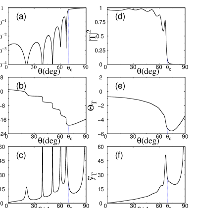
Figure 4: (Color online). The left column contains (a) $\left|R_{1}\right|^{2}$, (b) $\Theta_{1}^{R}$, and (c) $\tilde{y}_{R}$ as functions of $\theta$.  The right column contains (d) $\left|T_{1}\right|^{2}$, (e) $\Theta_{1}^{T}$, and (c) $\tilde{y}_{T}$ as functions of $\theta$ under the condition that $\tilde{\Delta}=200$ and the rest parameters are the same as in Fig. 2.

V Conclusion

In conclusion, we have established a theoretical framework for studying the matter wave analog of Goos-Hänchen-like effect in an atom optics model where a super-Gaussian laser beam acts as a ”medium slab” for a matter wave of two-level atoms.  We have developed  a vector theory based upon a set of coupled Schrödinger equations for describing the scattering of a wavepacket of two-level atoms off a square potential. We have derived a set of analytical formulas for the transmission and reflection coefficients, which have greatly facilitated the study of Goos-Hänchen effect in vector models where atoms are treated as particles possessing two internal spin components.   It is important to stress that the coupling between the ground and excited components in the vector model combined with the tunability offered by the laser field creates new opportunities for studying the lateral shifts.  In particular, we have found that in our atom optics model, not only a large negative Goos-Hänchen shift as in conventional optics WangLG:3 ; Lai:1 ; Shen ; Yan but also a large positive shift can take place in the reflected atomic beam.

VI Acknowledgements

We thank H. Pu for helpful discussion. This work is supported by the National Natural Science Foundation of China under Grant No. 10588402 and No. 10474055, the National Basic Research Program of China (973 Program) under Grant No. 2006CB921104, the Science and Technology Commission of Shanghai Municipality under Grant No. 06JC14026, No. 05PJ14038, the Program for Changjiang Scholars and Innovative Research Team in University, Shanghai Leading Academic Discipline Project No. B408, the Research Fund for the Doctoral Program of Higher Education No. 20040003101, and by the US National Science Foundation and the US Army Research Office (HYL).

Appendix A Appendix

In this Appendix, we provide the steps leading to Eqs. (35) and (36).  To begin with, we insert, $A_{i}=\frac{1}{2}\left(u_{i}+\frac{v_{i}}{\alpha_{i}}\right)e^{-\alpha_{i}L/2}$and $B_{i}=\frac{1}{2}\left(u_{i}-\frac{v_{i}}{\alpha_{i}}\right)e^{\alpha_{i}L/2}$ obtained from Eqs. (32), into Eqs. (34), enabling us to express $\left(x_{i}\text{,}y_{i}\right)$ in terms of ($u_{i}$, $v_{i}$) as

$$x_{i} =u_{i}\cosh\left(\alpha_{i}L\right)-v_{i}\sinh\left(\alpha_{i}L\right)/\alpha_{i},$$ (38a)

$$y_{i} =v_{i}\cosh\left(\alpha_{i}L\right)-\alpha_{i}u_{i}\sinh\left(\alpha_{i}L\right).$$ (38b)

By combining Eq. (33e) and Eq. (33j), we eliminate $R_{1}$ and $R_{2}$ simultaneously from Eqs. (33) and arrive at a single-matrix equation

$$U\left(\begin{array}[c]{c}x_{1}\\ x_{2}\end{array}\right)+W\left(\begin{array}[c]{c}y_{1}\\ y_{2}\end{array}\right)=\left(\begin{array}[c]{c}2e^{-ik_{1}L/2}\\ 0\end{array}\right),$$ (39)

which, by virtue of Eqs. (31) and (38), is shown to be equivalent to

$$M^{\left(+\right)}\left(\begin{array}[c]{c}T_{1}e^{ik_{1}L/2}\\ T_{2}e^{ik_{2}L/2}\end{array}\right)=\left(\begin{array}[c]{c}2e^{-ik_{1}L/2}\\ 0\end{array}\right),$$ (40)

where $M^{\left(+\right)}$ is a $2\times 2$ matrix given by

$$M^{\left(\pm\right)} =U\left[\begin{array}[c]{cc}\cosh\left(\alpha_{1}L\right)&0\\ 0&\cosh\left(\alpha_{2}L\right)\end{array}\right]U^{-1}-U\left[\begin{array}[c]{cc}\sinh\left(\alpha_{1}L\right)/\alpha_{1}&0\\ 0&\sinh\left(\alpha_{2}L\right)/\alpha_{2}\end{array}\right]W^{-1}$$ (45)

$$\pm W\left[\begin{array}[c]{cc}\cosh\left(\alpha_{1}L\right)&0\\ 0&\cosh\left(\alpha_{2}L\right)\end{array}\right]W^{-1}\mp W\left[\begin{array}[c]{cc}\alpha_{1}\sinh\left(\alpha_{1}L\right)/&0\\ 0&\alpha_{2}\sinh\left(\alpha_{2}L\right)\end{array}\right]U^{-1}.$$ (50)

By a similar procedure, we find from Eq. (33) that

$$2\left(\begin{array}[c]{c}R_{1}e^{ik_{1}L/2}\\ R_{2}e^{ik_{2}L/2}\end{array}\right)=U\left(\begin{array}[c]{c}x_{1}\\ x_{2}\end{array}\right)-W\left(\begin{array}[c]{c}y_{1}\\ y_{2}\end{array}\right),$$ (51)

which, with the help of Eqs. (31) and (38), is equivalent to

$$\left(\begin{array}[c]{c}2R_{1}e^{ik_{1}L/2}\\ 2R_{2}e^{ik_{2}L/2}\end{array}\right)=M^{\left(-\right)}\left(\begin{array}[c]{c}T_{1}e^{ik_{1}L/2}\\ T_{2}e^{ik_{2}L/2}\end{array}\right),$$ (52)

where $M^{\left(-\right)}$ is also $2\times 2$ matrix given by Eq. (50).  A straightforward calculation involving the use of Eq. (30) shows that the matrix element $M_{ij}^{\left(\pm\right)}$ of Eq. (50) has a simple and explicit form given by Eq. (37). Finally, we arrive at Eqs.(35) and (36) by solving Eqs. (40) and (52) simultaneously.

*wpzhang@phy.ecnu.edu.cn

† ling@rowan.edu

References

- (1) F. Goos and H. Hänchen, Ann. Phys. 1, 333 (1947); F. Goos and H. Hänchen, Ann. Phys. 5, 251 (1949).
- (2) K. Artmann, Ann. Phys. 2, 87 (1948).
- (3) A. M. Steinberg and R. Y. Chiao, Phys. Rev. A 49, 3283 (1994).
- (4) C. F. Li, Phys. Rev. Lett. 91, 133903 (2003).
- (5) L. G. Wang and S. Y. Zhu, Opt. Lett. 31, 101 (2006).
- (6) Y. Xiang, X. Dai, and S. Wen, Appl. Phys. A 87, 285 (2007).
- (7) L. Zeng and R. Song, Phys. Lett. A 358, 484 (2006).
- (8) R. H. Renard, J. Opt. Soc. Am. 54, 1190 (1964).
- (9) T. Tamir, J. Opt. Soc. Am. A 3, 558 (1986).
- (10) W. J. Wild and C. L. Giles, Phys. Rev. A 25, 2099 (1982).
- (11) R. Schlesser and A. Weis, Opt. Lett. 17, 1015 (1992).
- (12) E. Pfleghaar, A. Marseille, and A. Weis, Phys. Rev. Lett. 70, 2281 (1993).
- (13) H. M. Lai, S. W. Chan, and W. H. Wong J. Opt. Soc. Am. A 23, 3208 (2006).
- (14) C. Bonnet, D. Chauvat, O. Emile, F. Bretenaker, and A. Le Floch, Opt. Lett. 26, 666 (2001).
- (15) H. M. Lai and S. W. Chan, Opt. Lett. 27, 680 (2002).
- (16) P. R. Berman, Phys. Rev. E 66, 067603 (2002).
- (17) J. Broe and O. Keller, J. Opt. Soc. Am. A 19, 1212 (2002)
- (18) J. A. Kong, B.-L. Wu, and Y. Zhang, Appl. Phys. Lett. 80, 2084 (2002).
- (19) J. Fan, A. Dogariu, L. J. Wang, Opt. Express 11, 299 (2003).
- (20) N. F. Declercq, J. Degrieck, R. Briers, and O. Leroy, Appl. Phys. Lett. 82, 2533 (2003).
- (21) A. Lakhtakia, Electromagnetics 23, 71 (2003).
- (22) I. V. Shadrivov, A. A Zharov, and Y. S. Kivshar, Appl. Phys. Lett. 83, 2713 (2003).
- (23) Didier Felbacq and Rafik Smaâli, Phys. Rev. Lett. 92, 193902, (2004).
- (24) D.-K. Qing and G. Chen, Opt. Lett. 29, 872 (2004).
- (25) X. Chen and C.-F. Li, Phys. Rev. E 69, 066617 (2004).
- (26) L. G. Wang, H. Chen, and S. Y. Zhu, Opt. Lett. 30, 2936 (2005).
- (27) L. G. Wang and S. Y. Zhu, J. Appl. Phys. 98, 043522 (2005).
- (28) N. H. Shen, et al, Opt. Express 14, 10574 (2006).
- (29) X. B. Liu, Z. Q. Cao, P. F. Zhu, Q. S. Shen, and X. M. Liu, Phys. Rev. E 73, 056617 (2006).
- (30) J. He, J. Yi and S. He, Opt. Express 14, 3024 (2006).
- (31) K. L. Tsakmakidis, A. D. Boardman and O. Hess, Nature 450, 397 (2007)
- (32) Y. Yan, X. Chen, and C. F. Li, Phys. Lett. A 361 178 (2007).
- (33) S. C. Miller and N. Ashby, Phys. Rev. Lett. 29, 740 (1972).
- (34) D. M. Fradkin and R. J. Kashuba, Phys. Rev. D 9, 2775 (1974).
- (35) M. Mâaza, B. Pardo, Opt. Commun. 142, 84 (1997).
- (36) V.K. Ignatovich, Phys. Lett. A 322, 36 (2004).
- (37) Pierre Meystre, Atom Optics, Spinger-Verlag New York, Inc. (2001).
- (38) Weiping Zhang and B. C. Sanders, J. Phys. B 27, 795 (1994).
- (39) G. J. Dong, S. Edvadsson, W. Lu, and P. F. Barker, Phys. Rev. A 72, 031605(R) (2005).
- (40) J. S. Liu and M. R. Taghizadeh, Opt. Lett. 27, 1463 (2002).
- (41) P. A. Bélanger, R. L. Lachance, and C. Paré, Opt. Lett. 17, 739 (1992).
- (42) Y. Q. Zhao, Y. P. Li, and Q. G. Zhou, Opt. Lett. 29, 664 (2004).
- (43) E. T. Jaynes, F. W. Cummings, Proc IEEE 51, 89 (1963).
- (44) F. Delgado, J. G. Muga, and A. Ruschhaupt, Phys. Rev. A, 69 022106 (2004).