]http://www.iop.kiev.ua/ obraun

Modeling friction on a mesoscale: Master equation for the earthquake-like model

Abstract

The earthquake-like model with a continuous distribution of static thresholds is used to describe the properties of solid friction. The evolution of the model is reduced to a master equation which can be solved analytically. This approach naturally describes stick-slip and smooth sliding regimes of tribological systems within a framework which separates the calculation of the friction force from the studies of the properties of the contacts.

In spite of its crucial practical importance, friction is still not fully understood P0 . It raises questions at many scales, from the atomic scale studied nowadays by atomic force microscopy to the macroscopic scale of a solid block sliding on an other. A simple mesoscopic model has been introduced to bridge the gap in scales and describe the main experimental observations, such as stick slip or smooth sliding, in terms of the properties of local contacts. This widely used Burridge-Knopoff spring-block model BK1967 , initially introduced to study earthquakes (EQ model), has been developed by Olami, Feder and Christensen OFC1992 . It describes the contacts in terms of elastic springs and junctions that break at a critical force. Computer simulations P1995 ; BR2002 showed that the EQ model may reproduce the experimentally the observed stick-slip and smooth-sliding regimes, including the role of velocity and temperature, if the model is at least two-dimensional and various assumptions on the properties of the contacts are made.

The drawback of such a simulation approach is that heavy calculations with different parameter sets or contact properties are required to determine the main features of the model, and it is hard to draw conclusions of general validity. The calculations may be tedious because a large number of contacts and investigations on very long evolution times are necessary to get meaningful statistics and to make sure that the calculation has reached asymptotic properties which are not influenced by the initial conditions. Moreover almost all the studies based on the EQ model assume for simplicity, and to reduce the parameter space to explore, that all contacts have identical properties. It turns out that, as we show below, this limit is singular and may lead to qualitatively incorrect conclusions.

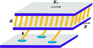
Figure 1: (color online): The earthquake-like model of friction.

Here we introduce a master equation (ME) approach which is much more efficient than simulations and can be solved analytically in cases which are particularly relevant. It provides a deeper understanding of friction analyzed at the mesoscale in terms of the statistical properties of the contacts. This splits the study of friction in two independent parts: (i) the calculation of the friction force given by the master equation provided the statistical properties of the contacts are known, (ii) the study of the contacts and their statistics, which needs inputs from the microscopic scale. Many aspects such as the interaction between the contacts and their aging can be studied separately to determine their role on the statistical properties of the contacts and then accounted for by the master equation approach.

Earthquake-like model. The EQ model describes the contact interface, i.e. the interface between the bottom of the solid block and the fixed substrate (Fig. 1). It assumes that the interaction occurs through $N_{c}$ asperities that make contacts with the substrate. Each asperity is characterized by its contact area $A_{i}$ and an elastic constant $k_{i}$, schematized by an elastic spring on Fig. 1, which can be estimated from $k_{i}\sim\rho\,c^{2}\sqrt{A_{i}}$, where $\rho$ is the mass density and $c$ is the transverse sound velocity of the material which forms the asperity P1995 . When the bottom of the solid block is moved by $X$, the stretching $x_{i}$ of an asperity, i.e. its elastic deformation with respect to its relaxed shape, increases. The force at the contact grows as $f_{i}=k_{i}x_{i}$ until it reaches the threshold value $f_{si}\propto A_{i}$ at $x_{si}=f_{si}/k_{i}\propto\sqrt{A_{i}}$; at this point the contact rapidly slides, and $f_{i}$ and $x_{i}$ drop to a small value before a contact is formed again.

Let $P_{c}(x_{s})$ be the normalized probability distribution of values of the thresholds $x_{si}$ at which contacts break. The model is studied in the quasi-static limit where inertia effects are neglected so that only positive values of $x_{i}$ are relevant. The distribution $P_{c}(x)$ can be characterized by its average value $\bar{x}_{s}$ and standard deviation $\sigma_{s}$. A typical example is a Gaussian distribution $P_{c}(x)=G(x;\bar{x},\sigma)$ note1 .

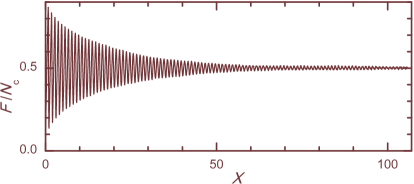
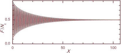
Figure 2: (a) Evolution of the EQ model. The curves show the distribution $Q(x;X)$ for incrementally increasing values of $X$ (with the step $\Delta X\approx 1$). The distribution $P_{c}(x)$ is Gaussian with $\bar{x}_{s}=1$ and $\sigma_{s}=0.05$, the initial distribution $Q_{\rm ini}(x)$ is Gaussian with $\bar{x}_{\rm ini}=0.1$ and $\sigma_{\rm ini}=0.025$. (b) Solution of the master equation with the increment $\Delta X=1.09$ for the same model parameters. The bottom panels show the corresponding dependences $F(X)$ for $\langle k_{i}\rangle=1$ and $K=\infty$.

To describe the evolution of the model, we introduce the distribution $Q(x;X)$ of the stretchings $x_{i}$ when the bottom of the solid block is at a position $X$. It is normalized by $\int_{0}^{\infty}dx\,Q(x;X)=1$ for all $X$. Let all asperities be initially relaxed or weakly stressed, e.g., let the distribution $Q(x;0)=Q_{\rm ini}(x)$ be the Gaussian $Q_{\rm ini}(x)=G(x;\bar{x}_{\rm ini},\sigma_{\rm ini})$ with $\bar{x}_{\rm ini}\ll\bar{x}_{s}$ and $\sigma_{\rm ini}\lesssim\sigma_{s}$. Now, let us adiabatically increase the displacement $X$ of the bottom of the solid block while the substrate remains fixed. The sum of the elastic forces exerted on the bottom of the block by the stretched asperities makes up the friction force

$$F(X)=N_{c}\langle k_{i}\rangle\int_{0}^{\infty}x\,Q(x;X)dx\;.$$ (1)

The evolution of the system, deduced from the numerical simulation of the EQ model is shown in Fig. 2a. It shows that, in the long term, the initial distribution approaches a stationary distribution $Q_{s}(x)$ and the total force $F$ becomes independent on $X$. The final distribution is independent of the initial one. An elegant mathematical proof of this statement was presented in Ref. FDW2005 . The statement is valid for any distribution $P_{c}(x)$ except for the singular case of $P_{c}(x)=\delta(x-x_{s})$.

Master equation. Rather than studying the evolution of the distribution $Q(x;X)$ by a simulation of the EQ model it is possible to describe it analytically. Let us consider a small displacement $\Delta\!X$ of the bottom of the solid block. It induces a variation of the stretching $x_{i}$ of the asperities which has the same value $\Delta\!X$ for all asperities if the deformation of the bottom surface of the block can be neglected. As discussed below, the general case where the relative positions of the asperities on the surface are allowed to vary can be cast into a generalization of this formalism. The displacement $X$ leads to three kinds of changes in the distribution $Q(x;X)$: first, there is a shift due to the global increase of the stretching of the asperities, second, some contacts break because the stretching exceeds the maximum that they can stand, and third, those broken contacts form again, at a lower stretching, after a slip at the scale of the asperities, which locally reduces the tension within the corresponding asperities. These three contributions can be written as a master equation for $Q(x;X)$:

$$Q(x;X+\Delta\!X)=Q(x-\Delta\!X;X)-\Delta Q_{-}(x;X)+\Delta Q_{+}(x;X).$$ (2)

The first term in the r.h.s. of Eq. (2) is just the shift. The second term $\Delta Q_{-}(x;X)$ designates the variation of the distribution due to the breaking of some contacts. It can be written as

$$\Delta Q_{-}(x;X)=P(x)\,\Delta\!X\,Q(x;X)\;,$$ (3)

where $P(x)\,\Delta\!X$ is the fraction of contacts that break when the position changes from $X$ to $X+\Delta\!X$. According to the definition of $P_{c}(x)$ the total number of unbroken contacts when the stretching of the asperities is equal to $x$ is given by $N_{c}\int_{x}^{\infty}P_{c}(\xi)\;d\xi$. The contacts that break when $X$ increases by $\Delta X$, so that the stretching of all asperities increases by $\Delta X$, is the number of contacts which have their thresholds between $x$ and $x+\Delta X$, i.e. $N_{c}P_{c}(x)\Delta X$. Thus

$$P(x)=P_{c}(x)\Big{/}\int_{x}^{\infty}d\xi P_{c}(\xi)\;.$$ (4)

The broken contacts relax and have to be added to the distribution around $x\sim 0$, leading to the third term in Eq. (2). We denote by $R(x)$ the normalized distribution of stretchings for the relaxed contacts. Writing that all broken contacts described by $\Delta Q_{-}(x;X)$ reappear with the distribution $R(x)$, we get

$$\Delta Q_{+}(x;X)=R(x)\int_{0}^{\infty}d\xi\,\Delta Q_{-}(\xi;X).$$ (5)

Equation (2) can be rewritten as $[Q(x;X+\Delta\!X)-Q(x;X)]+[Q(x;X)-Q(x-\Delta\!X;X)]=-\Delta Q_{-}(x;X)+\Delta Q_{+}(x;X)$. Taking the limit $\Delta\!X\to 0$, we finally get the integro-differential equation

$$\frac{\partial Q(x;X)}{\partial x}+\frac{\partial Q(x;X)}{\partial X}+P(x)\,Q(x;X)$$

$$=R(x)\int_{0}^{\infty}d\xi\,P(\xi)\,Q(\xi;X),$$ (6)

which has to be solved with the initial condition $Q(x;0)=Q_{\rm ini}(x)$. Notice that $Q_{\rm ini}(x)$ cannot be an arbitrary function, because the contacts that exceed their stability threshold, must relax from the very beginning.

Once the distribution $Q(x;X)$ is known, we can calculate the friction force $F(X)$ from Eq. (1). The static friction force is the maximum of $F(X)$, i.e., $F_{s}=F(X_{s})$, where $X_{s}$ is a solution of the equation $F^{\prime}(X)\equiv dF(X)/dX=0$. In order to simplify the calculation, we will assume in what follows that $R(x)=\delta(x)$, i.e. when the broken contacts stick again the asperities are completely relaxed.

Analytical solutions of the master equation can be obtained for some particular cases of contact properties BPnext , such as a rectangular $P_{c}(x)$ distribution. Moreover, for one particular but important choice of the initial distribution, when all contacts are relaxed at the beginning, $Q_{\rm ini}(x)=\delta(x)$, we can find analytically the initial part of the solution in a general case BPnext . For the rather general case of a Gaussian distribution of thresholds, $P_{c}(x)=G(x;\bar{x}_{s},\sigma_{s})$, a numerical solution of the master equation (6) is presented in Fig. 2b. One can see that it is almost identical to that of the EQ model (Fig. 2a), except for the noise on the EQ distributions. The distribution $Q(x;X)$ always approaches a stationary distribution $Q_{s}(x)$. The final distributions of the EQ model and the master equation approach are compared in Fig. 3.

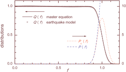
Figure 3: (color online): The final distribution $Q(x)$ for the parameters from Fig. 2 (solid curve; crosses show the averaged final distribution for the EQ model). The red dotted curve shows the distribution $P_{c}(x)$, and the blue broken curve shows $P(x)$.

The steady-state, or smooth-sliding solution, i.e. the solution of Eq. (6) which does not depend on $X$, can easily be found P1995 . In a general case it can be expressed as

$$Q_{s}(x)=C^{-1}\Theta(x)E_{P}(x),$$ (7)

where $\Theta(x)$ is the Heaviside step function, $E_{P}(x)=e^{-U(x)}$, $U(x)=\int_{0}^{x}d\xi\,P(\xi)$, and $C=\int_{0}^{\infty}dx\,E_{P}(x)$. The (kinetic) friction force is then equal to

$$F=(N_{c}/C)\langle k_{i}\rangle\int_{0}^{\infty}dx\,xE_{P}(x).$$ (8)

In the general case, let the distribution $P_{c}(x)$ be of bell-like shape with the maximum at $\bar{x}_{s}$ and the width $\sigma_{s}$. When $X$ shifts for the distance $\bar{x}_{s}$, due to the breaking and reforming of contacts with a lower stretching, an initially peaked distribution $Q(x;X)$ broadens by the value $\sim\sigma_{s}$ (Fig. 2). Therefore, any initial distribution tends to the stationary one as $|Q(x;X)-Q_{s}(x)|\propto\exp(-X/X^{*})$, where $X^{*}\sim\bar{x}_{s}^{2}/\sigma_{s}$.

Thus, in a general case the solution of the master equation always approaches the smooth-sliding one given by Eq. (7). However, there is one exception from this general scenario. When all contacts are identical, i.e., all contacts are characterized by the same threshold $x_{s}$, $P_{c}(x)=\delta(x-x_{s})$, the model admits a periodic solution BPnext . This singular periodic solution has been found in simulations and analyzed as describing the stick slip BN2006 , but actually it is unphysical and ceases to exist as soon as non-equivalent contacts are considered, whatever their precise properties. As discussed below the stick slip can be deduced from the solution of the master equation, but its origin is different Caroli .

Stick slip and smooth sliding. The master equation allows us to compute the friction force $F(X)$ when the bottom of the solid block is displaced by $X$. But actually we don’t control $X$. The displacement is caused by a shearing force $F_{T}$ applied on the top of the solid block which displaces the top surface by $X_{T}$. As the strain on the solid is generally small the deformation of the solid block can be assumed to be elastic so that $X_{T}$ is related to the applied force by $F_{T}=K(X_{T}-X)$ where $K$ is the shear elastic constant of the solid block. The total force applied to the bottom of the solid block, which determines its displacement $X$, is the sum of the applied force and the friction force

$$F_{\rm tot}=K(X_{T}-X)-F(X)\;.$$ (9)

It can be viewed as deriving from the potential

$$V(X_{T},X)=\frac{1}{2}K\,(X_{T}-X)^{2}+\int_{0}^{X}F(\xi)d\xi\;,$$ (10)

which determines the behavior of the solid block subjected to friction and applied force. A necessary condition for smooth sliding is that $X_{T}$ and $X$ grow together with $X_{T}-X=B$, where $B$ is a constant that measures the shear strain of the solid block during the sliding. It is determined by the condition ${\partial V}/{\partial(X_{T}-X)}=-{\partial V}/{\partial X}=0\;$ , which simply means that the total force on the interface vanishes. Smooth sliding also requires this state be stable,

$$\dfrac{\partial^{2}V}{\partial(X_{T}-X)^{2}}=\dfrac{\partial^{2}V}{\partial X^{2}}\geq 0\quad{\mathrm{or}}\quad F^{\prime}(X)\geq-K\;.$$ (11)

If we start from relaxed asperities, in the early stage of the motion $F(X)$ is a growing function of $X$, and then it passes by a maximum when some contacts start to break and reform at lower asperity stress. As a result $F^{\prime}(X)$ becomes negative. Depending on the value of $K$ two situations are possible. For large $K$ (stiff block) $F^{\prime}(X)$ never falls below $-K$ and the smooth sliding is a stable steady state. For small $K$ (soft block) $F^{\prime}(X)$ can become smaller than $-K$ so that the stability condition (11) is no longer valid. The instability causes $X_{T}-X$ to change abruptly by a breaking of all the contacts and a quick slip of the block before the contacts reform with relaxed asperities. And the process can repeat again, leading to the familiar stick slip motion. The master equation, which gives $F(X)$ can be used to compute the period of the stick slip, and, when the asperities fully relax before the contacts reform, an analytical solution can be obtained BPnext . It should be noticed that the existence of a stick slip is not only determined by the stiffness $K$ of the solid block. The properties of the asperities, defined by the distribution $P_{c}(x)$ of the stretching for which they break is also essential because it determines the expression of $F(X)$ and hence the minimal value of $F^{\prime}(X)$.

Discussion. The ME formalism can be extended to take into account various generalizations of the EQ model. For instance, in establishing the master equation we assumed that the asperities were fixed with respect to the solid block and were moving together with it. This is an approximation and one can, in principle, take into account the elastic deformation of the interface by introducing for instance a position dependent distribution $Q[x,X(\vec{r})]$ where $\vec{r}$ denotes the position of an asperity on the interface, and $X(\vec{r})$ the local translation of the interface averaged over a mesoscopic scale. The master equation must then be coupled to an equation describing the elastic deformation of the interface, subjected to the contact forces at each point $\vec{r}$. This illustrates the new viewpoint introduced by the ME approach which describes the phenomena at an intermediate scale between the microscopic scales of the contacts and the macroscopic scale of the displacement of the solid block. The ME equation only has a meaning if, on this intermediate scale, there are many individual contacts, allowing us to study them as a statistical distribution and not individually. A simpler view of the effect of the elastic interaction between the contacts is to describe it as a renormalization of the distribution $P_{c}(x)$ in a mean field like approach.

Another aspect which can be introduced in the ME formalism is the aging of the contacts BPnext . Experiments and MD simulations show that the static friction force grows with time since a contact is formed. As a result, if newly formed contacts are characterized by a distribution $P_{ci}(x)$ this distribution evolves with time, moving to a higher mean value and a smaller standard deviation. Aging is a stochastic process which can be described by a Smoluchowsky equation. The master equation for $Q(x,X)$ must then be completed by an equation for the evolution of $P_{c}(x)$, which in turns affects $P(x)$ in the master equation. Time enters through the velocity of the sliding, a faster sliding giving less time for the aging of the contacts. The full development is too long to be given here BPnext but it is easy to realize that a larger velocity leads to a smaller friction force because the contacts have less time to age, which is the source of a potential instability. Aging is therefore another cause for the stick-slip behavior.

The ME formalism can also accommodate temperature effects which enter again through their effect on the distribution $P(x)$ because thermal fluctuations allow an activated breaking of contacts for asperities which are still below their thresholds P1995 . The main point that we would like to stress is that this formalism introduces a new viewpoint on the mescoscopic modeling of friction. Moreover it splits the analysis of friction phenomena into problems that can be studied separately, the statistical properties of the contacts, and the evolution of the distribution $Q$ which is described by the master equation, coupled to additional equations representing different effects such as the elastic interactions between asperities, the aging of the contacts or temperature fluctuations.

This work was supported by CNRS-Ukraine grant No. 18977. O.B. acknowledges a partial support from the EU Exchange Grant within the ESF program “Nanotribology” (NANOTRIBO).

References

- (1) B. N. J. Persson, Sliding Friction: Physical Principles and Applications (Springer-Verlag, Berlin, 1998).
- (2) R. Burridge and L. Knopoff, Bull. Seismol. Soc. Am. 57, 341 (1967).
- (3) Z. Olami, H. J. S. Feder, and K. Christensen, Phys. Rev. Lett. 68, 1244 (1992).
- (4) B.N.J. Persson, Phys. Rev. B51, 13568 (1995).
- (5) O.M. Braun and J. Röder, Phys. Rev. Lett. 88, 096102 (2002).
- (6) More rigorously, the distribution should be truncated to be defined on the interval , where
- (7) Z. Farkas, S.R. Dahmen, and D.E. Wolf, J. Stat. Mech.: Theory and Experiment P06015 (2005); cond-mat/0502644. The authors considered a simplified version of EQ model, assuming that every contact keeps its own threshold value unchanged after breaking/reforming.
- (8) O.M. Braun and M. Peyrard, unpublished.
- (9) O.M. Braun and A. Naumovets, Surf. Sci. Reports 60, 79-158 (2006)
- (10) T. Baumberger and C. Caroli, Advances in Physics 55 279-348 (2006)