Pair Partitioning in time reversal acoustics

Abstract

Time reversal of acoustic waves can be achieved efficiently by the persistent control of excitations in a finite region of the system. The procedure, called Time Reversal Mirror, is stable against the inhomogeneities of the medium and it has numerous applications in medical physics, oceanography and communications. As a first step in the study of this robustness, we apply the Perfect Inverse Filter procedure that accounts for the memory effects of the system. In the numerical evaluation of such procedures we developed the Pair Partitioning method for a system of coupled oscillators. The algorithm, inspired in the Trotter strategy for quantum dynamics, obtains the dynamic for a chain of coupled harmonic oscillators by the separation of the system in pairs and applying a stroboscopic sequence that alternates the evolution of each pair. We analyze here the formal basis of the method and discuss his extension for including energy dissipation inside the medium.

I Introduction

In the recent years, the group of M. Fink developed an experimental technique called Time Reversal Mirror (TRM) fink99 that allows time reversal of ultrasonic waves. An ultrasonic pulse is emitted from the inside of the control region (called cavity) and the excitation is detected as it escapes through a set of transducers placed at the boundaries. These transducers can act alternatively like microphones or loudspeakers and the registered signal is played back in the time reversed sequence. Thus, the signal focalizes in space and time in the source point forming a Loschmidt Echo jalabert01 . It is remarkable that the quality of focalization gets better by increasing the inhomogeneities inside the cavity. This property allows for applications in many fields fink03 ; edelman02 . In order to have a first formal description for the exact reversion, we introduced a time reversal procedure denoted Perfect Inverse Filter (PIF) in the quantum domain pastawski07 . The PIF is based in the injection of a wave function that precisely compensates the feedback effects by means of the renormalization of the registered signal in the frequency domain. This also accounts for the correlations between the transducers. Recently, we proved that these concepts apply for classical waves calvo07 . We applied it to the numerical evaluation of the reversal of excitations in a linear chain of classical coupled harmonic oscillators with satisfactory results. A key issue in assessing the stability of the reversal procedure is have a numerical integrator that is stable and perfectly reversible. Therefore, we developed a numerical algorithm, the Pair Partitioning method (PP), that allowed the precise test of the reversal procedure. In the next section we develop the main idea of the method and then we use it to obtain the numerical results that we compare with the analytical solution for the homogeneous system. Additionally, we introduce a method to approximate the solution of an infinite system using a finite one. For this we introduce a non-homogeneous fictitious friction term that can simulate the diffusion of the excitation occurring in an unbounded system. These strategies are tested through a numerical simulation of a time reversal experiment.

II Wave dynamics in the Pair Partitioning method

The system to be used is shown in the figure 1: a one-dimensional chain of $N=2s$ coupled oscillators with masses $m_{i}$ and natural frequencies $\omega_{i}$ that can be represented as a set of coupled pendulums.

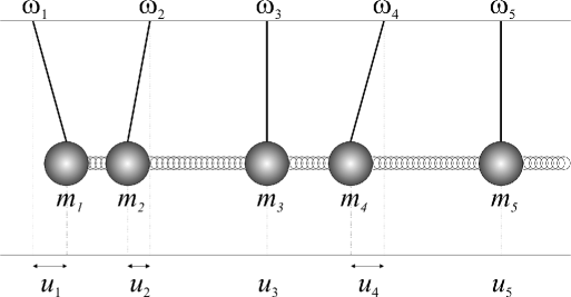
Figure 1: Scheme of the $N$ coupled oscillators system to be solved by the PP numerical method.

If $p_{i}$ denotes the impulse and $u_{i}$ the displacement amplitude from the equilibrium position for the $i$th oscillator, the Hamiltonian writes

$$\mathcal{H}=\sum_{i=1}^{N}\left(\frac{p_{i}^{2}}{2m_{i}}+\frac{m_{i}\omega_{i}^{2}}{2}u_{i}^{2}\right)+\sum_{i=1}^{N-1}\frac{K_{i}}{2}\left(u_{i+1}-u_{i}\right)^{2},$$ (1)

where $K_{i}$ is the elastic coefficient that accounts for the coupling between the oscillators $i$ and $i+1$. Notice that we could rewrite the Hamiltonian in terms of each coupling separating it in non-interacting terms including even pairs and odd pairs each:

$$\mathcal{H} =\mathcal{H}_{\mathrm{odd}}+\mathcal{H}_{\mathrm{even}}=\mathcal{H}_{1,2}+\mathcal{H}_{3,4}+\ldots+\mathcal{H}_{N-1,N}$$ (2)

$$+\mathcal{H}_{2,3}+\mathcal{H}_{4,5}+\ldots+\mathcal{H}_{N-2,N-1},$$

with

$$\mathcal{H}_{n,n+1}=\frac{p_{n}^{2}}{2\tilde{m}_{n}}+\frac{\tilde{m}_{n}\tilde{\omega}_{n}^{2}}{2}u_{n}^{2}+\frac{p_{n+1}^{2}}{2\tilde{m}_{n+1}}+\frac{\tilde{m}_{n+1}\tilde{\omega}_{n+1}^{2}}{2}u_{n+1}^{2}+\frac{K_{n}}{2}\left(u_{n+1}-u_{n}\right)^{2},$$ (3)

and

$$\tilde{m}_{1} =m_{1},\ \tilde{\omega}_{1}=\omega_{1},\ \tilde{m}_{N}=m_{N},\ \tilde{\omega}_{N}=\omega_{N},$$ (4)

$$\tilde{m}_{n} =2m_{n},\ \tilde{\omega}_{n}=\omega_{n}/2,\ n=2,\ldots,N-1.$$

A good approximation to the overall dynamics, inspired in the Trotter method used in quantum mechanics deraedt96 , can be obtained solving analytically the equations of motion for each independent Hamiltonian in a time step $\tau$. Therefore, the pair $\mathcal{H}_{n,n+1}$ has

$$\ddot{u}_{n} =-\left(\tilde{\omega}_{n}^{2}+\frac{K_{n}}{\tilde{m}_{n}}\right)u_{n}+\frac{K_{n}}{\tilde{m}_{n}}u_{n+1},$$ (5)

$$\ddot{u}_{n+1} =-\left(\tilde{\omega}_{n+1}^{2}+\frac{K_{n}}{\tilde{m}_{n+1}}\right)u_{n+1}+\frac{K_{n}}{\tilde{m}_{n+1}}u_{n}.$$

At each small time step $\tau$, the evolution for the even couplings is obtained and the resulting positions and velocities are used as initial conditions for the set of Hamiltonians accounting for odd couplings and so on. Since the equations of motion are solved separately, we could consider only the two coupled oscillators system, e.g.

$$\ddot{u}_{1} =-\omega_{1}^{2}u_{1}+\omega_{12}^{2}u_{2},$$ (6)

$$\ddot{u}_{2} =-\omega_{2}^{2}u_{2}+\omega_{21}^{2}u_{1}.$$

For this system, it is easy to obtain the corresponding normal modes

$$U_{\pm}=\mp\frac{\omega_{21}^{2}}{\omega_{+}^{2}-\omega_{-}^{2}}u_{1}\pm\frac{\omega_{1}^{2}-\omega_{\mp}^{2}}{\omega_{+}^{2}-\omega_{-}^{2}}u_{2},$$ (7)

with characteristic frequencies

$$\omega_{\pm}^{2}=\frac{\omega_{1}^{2}+\omega_{2}^{2}}{2}\pm\sqrt{\left(\frac{\omega_{1}^{2}-\omega_{2}^{2}}{2}\right)^{2}+\omega_{12}^{2}\omega_{21}^{2}}.$$ (8)

From (7), $U_{\pm}(t)$ are obtained and these values are used for the evolution after the temporal step $t\rightarrow t+\tau$, i.e.

$$U_{\pm}(t+\tau) =U_{\pm}(t)\cos(\omega_{\pm}\tau)+\dot{U}_{\pm}(t)\sin(\omega_{\pm}\tau)/\omega_{\pm},$$ (9)

$$\dot{U}_{\pm}(t+\tau) =\dot{U}_{\pm}(t)\cos(\omega_{\pm}\tau)-U_{\pm}(t)\sin(\omega_{\pm}\tau)\omega_{\pm}.$$

Once we have $U_{\pm}(t+\tau)$ and $\dot{U}_{\pm}(t+\tau)$ we can go back to the natural basis by means of the inverse of (7)

$$u_{1} =\frac{\omega_{1}^{2}-\omega_{+}^{2}}{\omega_{21}^{2}}U_{+}+\frac{\omega_{1}^{2}-\omega_{-}^{2}}{\omega_{21}^{2}}U_{-},$$ (10)

$$u_{2} =U_{+}+U_{-}.$$

Then, one obtains the displacements and momenta for all oscillators at time $t+\tau$. The above steps are summarized in the Pair Partitioning algorithm:

1. Determine all the masses and natural frequencies of the partitioned system $\tilde{m}_{n},\tilde{\omega}_{n}$.

2. For even couplings $\mathcal{H}_{2,3},\mathcal{H}_{4,5},\ldots$, rewrite the initial conditions $\left\{u_{i}(0),\dot{u}_{i}(0)\right\}$ for the normal modes according to (7).

3. Calculate the normal modes evolution for even couplings, according to (9) and obtain $\left\{u_{i}^{\mathrm{even}}(\tau),\dot{u}_{i}^{\mathrm{even}}(\tau)\right\}$ from (10).

4. Calculate the normal modes for odd couplings $\mathcal{H}_{1,2},\mathcal{H}_{3,4},\ldots$, using the recent positions and velocities.

5. Calculate the normal modes evolution for odd couplings and give the positions and velocities $\left\{u_{i}(\tau),\dot{u}_{i}(\tau)\right\}$.

6. Go back to the step 2 with $\left\{u_{i}(\tau),\dot{u}_{i}(\tau)\right\}$.

Therefore, applying $n$ times the PP algorithm we obtain the positions and velocities for all oscillators at time $t=n\tau$.
As an example we consider the homogeneous system where the $N$ oscillators have identical masses and the only natural frequencies correspond to the surface $\omega_{1}=\omega_{N}=\omega_{\mathrm{x}}=\sqrt{K/m}$. The displacement amplitude of the $i$th oscillator due to an initial displacement in the $j$th oscillator can be expressed analytically as

$$u_{i\leftarrow j}^{\mathrm{th.}}(t)=\frac{2}{N+1}\sum_{k=1}^{N}\sin\left(i\frac{k\pi}{N+1}\right)\sin\left(j\frac{\pi}{N+1}\right)\cos(\omega_{k}t),$$ (11)

with

$$\omega_{k}=\omega_{\mathrm{x}}\sin\left(\frac{k\pi}{2(N+1)}\right),$$ (12)

the characteristic frequency for the $k$th normal mode. In the figure 2 the analytical and numerical results are compared for the surface oscillator displacement in a case when all the oscillators were initially in their equilibrium positions except $u_{1}(0)=u_{1}^{0}$. We use $N=200$ in two cases where the temporal steps are $\tau=10^{-2}\omega_{\mathrm{x}}^{-1}$ and $\tau=10^{-3}\omega_{\mathrm{x}}^{-1}$.

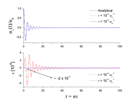
Figure 2: Time evolution for the surface oscillator. Top, comparison between the analytical and numerical results shows all curves superposed. Bottom, error in the displacement for both temporal steps.

We have taken $N$ such that no mesoscopics echoes pastawski95 appear in the interval of time shown. We also notice that the error

$$\varepsilon(t)=\frac{\left|u_{1}^{\mathrm{th.}}(t)-u_{1}^{\mathrm{PP}}(t)\right|}{u_{0}},$$ (13)

drops as the temporal step $\tau$ diminishes. We observe a quadratic dependence $\mathrm{\max}{\varepsilon(t)}=\alpha\tau^{2}$ in complete analogy with the Trotter method. In the particular case of the homogeneous system we have $\alpha\simeq 0.0445$.

II.1 Unbounded systems as damped oscillations

The solution of wave dynamics in infinite media remains as a delicate problem. In such case, the initially localized excitation spreads through the systems in a way that resembles actual dissipation. In contrast, finite systems present periodic revivals, the mesoscopic echoes, that show that energy remains in the system. In order to get rid the mesoscopic echoes and obtaining a form of “dissipation” using a finite number of oscillators, we add a fictitious “friction” term. The friction coefficients $\eta_{i}\geq 0$ can be included between the $2$th and $3$th steps of the PP algorithm supposing that the displacement amplitude decays exponentially

$$u_{i}(t)\rightarrow u_{i}(t)\exp(-\eta_{i}\tau),$$ (14)

as occurs in a damped oscillator in the limit $\eta/\omega\ll 1$. For the homogeneous system with $N=100$ oscillators were the cavity ending at site $x_{R}$ we choose a progressive increase in the damping as

$$\eta_{i}=0.1\frac{i-x_{R}}{N-x_{R}},\ i=x_{R},\ldots,N.$$ (15)

We compare the result of this approximation with the undamped case for the displacement amplitude in $x_{R}=10$. The figure 3 shows how the dynamics in the damped system has no mesoscopic echoes whereas in the undamped system we observe the echo at $t_{M}\simeq 2N\omega_{\mathrm{x}}^{-1}$.

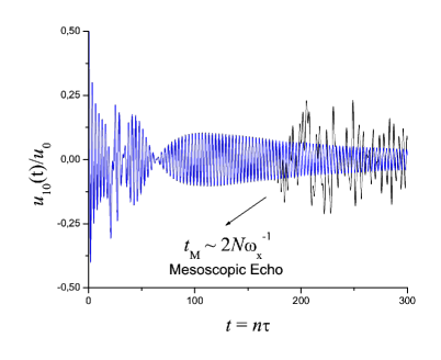
Figure 3: Comparison between the undamped evolution (black) and the damped evolution (blue) for the displacement amplitude $u_{R}(t)$.

As we will see for TRM and PIF procedures, this last result is very usefull since it allows to obtain the dynamics of an open system with a small number of oscillators (e.g. $N\simeq 100$).

III Numerical test for the Perfect Inverse Filter procedure

As we mentioned above, the Time Reversal Mirror procedure consists in the injection, at the boundaries of the cavity, of a signal proportional to that recorded during the forward propagation. In contrast, the Perfect Inverse Filter corrects this recorded signal to accounts for the contributions of multiple reflections and normal dispersion of the previously injected signal in a manner that their instantaneous total sum coincides precisely with the time reversed signal at the boundaries. The continuity of the wave equation ensures that perfect time reversal occurs at every point inside the cavity. The procedure for such correction is described somewhere else pastawski07 ; calvo07 . Here, it is enough to notice that the imposition of an appropriate wave amplitude at the boundaries should give the perfect reversal of an excitation originally localized inside the cavity. An example of such situation would be a “ surface pendulum” coupled to a semi-infinite linear chain of harmonically coupled masses calvo06 . In such a case, we know that the energy decays in a approximately exponential way, where the decay rate can be assimilated to a “friction coefficient ”. However, for very short times, the local energy decays with a quadratic law while for very long times the exponential decay gives rise to a power law characteristic of the slow diffusion of the energy rufeil06 . In the figure 4 we show how this overall decay is reversed by controling the amplitude at site $x_{R}=10$.

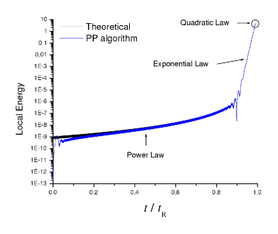
Figure 4: Local energy of the surface oscillator recovering. Here, we choose for the detection time $t_{R}=1000\tau$. evolution (blue) for the displacement amplitude $u_{R}(t)$.

As long as we have been able to wait until a neglegible amount of energy is left in the cavity, the control of the boundaries is enough to reverse the whole dynamics inside the cavity. As a comparison, the theoretical reversal of the decay of a surface excitation in a semi-infinite chain is shown. We see that the region they differ is when the injected signal is still negligible as compared to the energy still remaining in the cavity (as a concequence of the very slow power law decay).

IV Discussion

We have presented a numerical strategy for the solution of the wave equation that is completely time reversible. This involves the iterative application of the exact evolution of pairs of coupled effective oscillators where the energy is conserved, hence deserving the name of Pair Partitioning method. This is complemented with an original strategy for dealing with wave propagation through infinite media. While various tests of these procedures remain to be done, we have shown, through the solution of simple but highly non-trivial examples, that the method is numerically stable and can be used to revert wave dynamics up to a desired precision.

References

- (1) M. Fink, Time-reversed acoustics, Scientific American 281 (may), 91-97 (1999).
- (2) R.A. Jalabert and H.M. Pastawski, Environment-independent decoherence rate in classically chaotic systems, Physical Review Letters 86, 2490-2493 (2001).
- (3) M. Fink, G. Montaldo and M. Tanter, Time-reversal acoustics in biomedical engineering, Annual Reviews of Biomedical Engineering 5, 465-497 (2003).
- (4) G.F. Edelman, T. Akal, W.S. Hodkiss, S. Kim, W.A. Kuperman and H. C. Song, An initial demonstration of underwater acoustic communication using time reversal, IEEE Journal of Ocean Engineering 27 (3), 602-609 (2002).
- (5) H.M. Pastawski, E.P. Danieli, H.L. Calvo and L.E.F. Foa-Torres, Towards a time-reversal mirror for quantum systems, Europhysics Letters 77, 40001 (2007).
- (6) H.L. Calvo, E.P. Danieli and H.M. Pastawski, Time reversal mirror and perfect inverse filter in a microscopic model for sound propagation, Physica B 398 (2), 317-320 (2007).
- (7) H. deRaedt, Computer simulation of quantum phenomena in nanoscale devices, Annual Reviews of Computational Physics IV, 107-146 (1996).
- (8) H.M. Pastawski and P.R. Levstein and G. Usaj, Quantum dynamical echoes in the spin diffusion in mesoscopic systems, Physical Review Letters 75, 4310-4313 (1995).
- (9) H.L. Calvo and H.M. Pastawski, Dynamical phase transition in vibrational surface modes, Brazilian Journal of Physics 36 (3b), 963-966 (2006).
- (10) E. Rufeil Fiori and H.M. Pastawski, Non-Markovian decay beyond the Fermi Golden Rule: survival collapse of the polarization in spin chains, Chemical Physics Letters 420, 35-41 (2006).