Well-Posedness for the Euler-Nordström System with Cosmological Constant

Abstract.

In this paper the author considers the motion of a relativistic perfect fluid with self-interaction mediated by Nordström’s scalar theory of gravity. The evolution of the fluid is determined by a quasilinear hyperbolic system of PDEs, and a cosmological constant is introduced in order to ensure the existence of non-zero constant solutions. Accordingly, the initial value problem for a compact perturbation of an infinitely extended quiet fluid is studied. Although the system is neither symmetric hyperbolic nor strictly hyperbolic, Christodoulou’s constructive results on the existence of energy currents for equations derivable from a Lagrangian can be adapted to provide energy currents that can be used in place of the standard energy principle available for first-order symmetric hyperbolic systems. After providing such energy currents, the author uses them to prove that the Euler-Nordström system with a cosmological constant is well-posed in a suitable Sobolev space.

1. Introduction

It is well-known that for symmetric hyperbolic systems of PDEs, an energy principle is available that implies well-posedness (local existence, uniqueness, and continuous dependence on initial data) for initial data belonging to an appropriate Sobolev space. Consult [9], [10], [13], [21], [22], or [31] for the definition of a symmetric hyperbolic system and a detailed proof of local existence in this case. A full proof of well-posedness is difficult to locate in the literature, but Kato [18] supplies one using a very general setup that applies to symmetric hyperbolic systems in a Banach space. Additionally, for strictly hyperbolic (not necessarily symmetric) systems, well-posedness follows from the availability of a generalization of the energy principle for symmetric hyperbolic systems. For strictly hyperbolic systems, there are a variety of methods due to Petrovskii, Leray, G$\mathring{\mbox{a}}$rding, and Calderón for generating energy estimates; consult [9] or [21] for details on these methods.

We consider here the Cauchy problem for the Lorentz covariant Euler-Nordström (EN) system, which is a scalar caricature of the general covariant Euler-Einstein system describing a gravitationally self-interacting fluid. The EN system is a quasilinear hyperbolic system of PDEs that is not manifestly symmetric hyperbolic. Moreover, because of the repeated factors in the expression for $\mathcal{Q}(x;\cdot)$ in equation (5.1.7) below, and because the sheets of the characteristic subset of the cotangent space at $x$ intersect (see Fig. 1), it is not strictly hyperbolic. Therefore, well-posedness for the EN system does not follow from either of these two well-known frameworks.

Fortunately, alternate techniques recently developed by Christodoulou [6], and which are applied to the study of relativistic fluids in Minkowski spacetime in particular in [7], offer a viable approach to studying the Cauchy problem for the EN system. The central advantage afforded by Christodolou’s techniques, which provide energy currents for equations derivable from a Lagrangian, is that they bypass the physically artificial requirement of symmetry in the equations: even though the EN system is not manifestly symmetric, its energy currents allow for precisely the same energy estimates to be made as in the theory of symmetric hyperbolic systems. Once one has these estimates, the proof of well-posedness for the EN system mirrors the well known proof for symmetric hyperbolic systems. Our main goal is to use the method of energy currents to prove the following theorem (stated loosely here), which is divided into parts and stated rigorously in Section 7:

• Main Theorem (Well-Posedness).   Let $N\geq 3$ be an integer. Assume that the initial data $\mathring{\mathbf{V}}$ for the EN system are an $H^{N}$ perturbation of a constant background solution $\bar{\mathbf{V}}.$ Then these data launch a unique solution $\mathbf{V}$ possessing the regularity property $\mathbf{V}-\bar{\mathbf{V}}\in C_{b}^{1}([0,T]\times\mathbb{R}^{3})\cap C^{0}([0,T],H^{N})\cap C^{1}([0,T],H^{N-1}).$ Furthermore, the map from the initial perturbation $\mathring{\mathbf{V}}-\bar{\mathbf{V}}$ to $\mathbf{V}-\bar{\mathbf{V}}$ is a continuous map from an open subset of $H^{N}$ into $C^{0}([0,T],H^{N}).$

While Christodoulou’s methods are not the only techniques available for proving the well-posedness of the EN system, they are powerful and natural in the sense that they exploit the inherent geometry of the equations. In contrast, one may proceed by seeking a change of state-space variables that renders the system symmetric hyperbolic. For example, Makino applies this symmetrizing technique to the Euler-Poisson equations in [23], and Makino and Ukai apply it to the relativistic Euler equations without gravitational interaction in [24] and [25]. Further discussion of applications of symmetrization discussed in the literature can be found in sections 3.1 and 3.2. Yet the symmetrizing method is not without disadvantages: one must solve a formally over-determined system of equations to find the symmetrizing variables, and the resulting state-space variables, if they exist, may place un-physical and/or mathematically unappealing restrictions on the function spaces with which one would like to work. However, it should be noted that Makino’s symmetrization is currently capable of dealing with a restricted class of compactly supported data, while the techniques applied here cannot yet handle such data due to singularities in the energy current (5.5.1) when the proper energy density $\rho$ of the fluid vanishes.

2. Remarks on the Notation

We introduce here some notation that is used throughout this article, some of which is non-standard. We assume that the reader is familiar with standard notation for the $L^{p}$ spaces and the Sobolev spaces $H^{k}.$ Unless otherwise stated, the symbols $L^{p}$ and $H^{k}$ refer to $L^{p}(\mathbb{R}^{3})$ and $H^{k}(\mathbb{R}^{3})$ respectively.

2.1. Notation and assumptions regarding spacetime

In the Euler-Poisson system with cosmological constant introduced below, we use $t\in\mathbb{R}$ to denote the time variable and $\mathbf{s}\in\mathbb{R}^{3}$ to denote the space variable. In the Euler-Einstein and EN systems (which we also equip with a cosmological constant below), we assume that spacetime is a 4-dimensional, time-orientable Lorentzian manifold $\mathcal{M}$ and use the notation

(2.1.1) $$x=(x^{0},x^{1},x^{2},x^{3})$$

to denote spacetime points. For the EN system with cosmological constant, we assume the existence of a global system of rectangular coordinates (an inertial frame), and for this preferred time-space splitting, we identify $t=x^{0}$ with time and $\mathbf{s}=(x^{1},x^{2},x^{3})$ with space and use the notation (2.1.1) to denote the components of $x$ relative to this fixed coordinate system.

2.2. Notation regarding differential operators

If $F$ is a scalar or finite-dimensional array-valued function on $\mathbb{R}^{1+3},$ then $DF$ denotes the array consisting of all first-order spacetime partial derivatives (including the partial derivative with respect to time) of every component of $F,$ while $\nabla^{(a)}F$ denotes the array of consisting of all $a^{th}$ order spatial partial derivatives of every component of $F;$ this should not be confused with $\nabla,$ which represents covariant differentiation.

2.3. Index conventions

We adopt Einstein’s notation that repeated Latin indices are summed from $1\ \mbox{to}\ 3,$ while repeated Greek indices are summed from $0\ \mbox{to}\ 3.$ Indices are raised and lowered using a spacetime metric, which varies according to context.

2.4. Notation regarding norms and function spaces

If $\bar{\mathbf{V}}$ is a constant array, we use the notation

$$\|F\|_{L_{\bar{\mathbf{V}}}^{p}(\mathscr{A})}\overset{\mbox{\tiny{def}}}{=}\|F-\bar{\mathbf{V}}\|_{L^{p}(\mathscr{A})},$$

and we denote the set of all Lebesgue measurable functions $F$ such that
$\|F\|_{L_{\bar{\mathbf{V}}}^{p}(\mathscr{A})}<\infty$ by $L_{\bar{\mathbf{V}}}^{p}(\mathscr{A}).$ Unless we indicate otherwise, we assume that $\mathscr{A}=\mathbb{R}^{3}$ when the set $\mathscr{A}$ is not explicitly written.

If $F$ is a map from the interval $[T_{1},T_{2}]$ into the normed function space $X,$ we use the notation

$$\mid\mid\mid F\mid\mid\mid_{X,[T_{1},T_{2}]}\ \overset{\mbox{\tiny{def}}}{=}\underset{t\in[T_{1},T_{2}]}{\sup}\|F(t)\|_{X}.$$

We often abbreviate $\mid\mid\mid F\mid\mid\mid_{X,T}$ in place of $\mid\mid\mid F\mid\mid\mid_{X,[0,T]}.$

We also use the notation $C^{k}([0,T],X)$ to denote the set of $k$-times continuously differentiable maps from $(0,T)$ into $X$ that, together with their derivatives up to order $k,$ extend continuously to $[0,T].$

If $\mathscr{A}\subset\mathbb{R}^{d}$ ($d$ frequently equals $3,4,$ or $10$ in this article) and $\mathscr{A}$ is open, then $C^{k}_{b}(\bar{\mathscr{A}})$ denotes the set $k-$times continuously differentiable functions (either scalar or array-valued, depending on context) on $\mathscr{A}$ with bounded derivatives up to order $k$ that extend continuously to the closure of $\mathscr{A}.$ The norm of a function $F\in C^{k}_{b}(\bar{\mathscr{A}})$ is defined by

$$|F|_{k,\mathscr{A}}\overset{\mbox{\tiny{def}}}{=}\sum_{|\vec{\alpha}|\leq k}\sup_{z\in\mathscr{A}}|\partial_{\vec{\alpha}}F(z)|,$$

where $\partial_{\vec{\alpha}}$ represents differentiation with respect to the arguments $z$ of $F$ (which may be spacetime variables or state-space variables, depending on the context).

2.5. Notation regarding operators

If $X$ and $Y$ are normed function spaces, then $\mathcal{L}(X,Y)$ denotes the set of bounded linear maps from $X$ to $Y.$ If $\mathcal{U}\in\mathcal{L}(X,Y),$ then we denote its operator norm by $\|\mathcal{U}\|_{X,Y}.$ If $X=Y,$ we write $\mathcal{L}(X)$ instead of $\mathcal{L}(X,Y)$ and $\|\mathcal{U}\|_{X}$ instead of $\|\mathcal{U}\|_{X,X}.$ If $\mathcal{U}(t,t^{\prime})$ is an operator-valued map from the triangle
$\triangle_{T}\overset{\mbox{\tiny{def}}}{=}\{0\leq t^{\prime}\leq t\leq T\}$ into $\mathcal{L}(X),$ then we adopt the notation

$$\mid\mid\mid\mathcal{U}\mid\mid\mid_{X,\triangle_{T}}\overset{\mbox{\tiny{def}}}{=}\sup_{(t,t^{\prime})\in\triangle_{T}}\|\mathcal{U}(t,t^{\prime})\|_{X}.$$

2.6. Notation regarding constants

We use the symbol $C$ to denote a generic constant in the estimates below which is free to vary from line to line. If the constant depends on quantities such as real numbers $N^{\prime},$ subsets $\mathscr{A}$ of $\mathbb{R}^{d},$ functions $F$ of the state-space variables, etc., that are peripheral to the argument at hand, we sometimes indicate this dependence by writing $C(N^{\prime},\mathscr{A},F),$ etc. We frequently omit the dependence of $C$ on functions of the state-space variables below in order to conserve space, but we explicitly show the dependence when it is (in our judgment) illuminating. Occasionally, we shall use additional symbols such as $C_{\bar{\mathcal{O}}_{2}},L,K,$ etc., to denote constants that play a distinguished role in the discussion below.

3. The EN and EN_κ Models in Context

The EN system is an intermediate model in between the Galilean covariant Euler-Poisson (EP) and the general covariant Euler-Einstein (EE) systems for self-gravitating classical fluids. Although it is the most fundamental of these models for self-gravitating Eulerian fluids, the EE system presents numerous technical difficulties that make a detailed analysis of the system’s evolution, through either numerical or analytical methods, extremely difficult. For example, in General Relativity there is a coordinate gauge freedom due to the diffeomorphism covariance of the equations, and furthermore, there is no known law of local conservation of gravitational energy. Our main motivations for studying the EN system are to bridge the gap between the EP and the EE systems and to provide a special relativistic primer for studying the EE system.

Since it is based on Nordström’s theory of gravity, it should be stressed that the EN system is physically wrong. However, since both the EN and the EE systems are relativistic generalizations of the EP system, we expect, at least in some limiting cases, that there are some qualitative similarities between solutions to the three systems. Furthermore, in [32], Shapiro and Teukolsky discuss numerical simulations of the EN system in the spherically symmetric case; they expect that the numerical schemes developed in their paper can be adapted to allow for the calculation of accurate wave forms in the EE model.

Before discussing the EN system in detail, we briefly recall the EP and EE systems, endowing both with a cosmological constant denoted by $\kappa^{2}.$ We also briefly discuss some local existence proofs for these systems in the case $\kappa=0,$ emphasizing their dependence on the symmetric hyperbolic setup or the method of Leray (strict) hyperbolicity.

We introduce a positive cosmological constant out of mathematical necessity: the EN system fails to have non-zero constant solutions without it. Our reasoning is similar to the reasoning that led Einstein to introduce the cosmological constant into General Relativity; he sought a static universe, and General Relativity without a cosmological constant features only Minkowski space as a static homogeneous solution (see [12]). We emphasize the presence of the cosmological constant $\kappa^{2}$ in the models by referring to them as the EP${}_{\kappa},$ EE${}_{\kappa},$ and EN_κ systems; note that EP$=$EP${}_{0},$ and similarly for the other two models.

3.1. The Euler-Poisson system with cosmological constant (EP_κ)

In units with Newton’s universal gravitational constant equal to 1, the equations governing the dynamics in this case are

(3.1.1) $$\partial_{t}{{\eta}}+v^{k}\partial_{k}{{\eta}} =0$$

(3.1.2) $$\partial_{t}{\rho}+\partial_{k}(\rho v^{k}) =0$$

(3.1.3) $$\rho\left(\partial_{t}v_{j}+v^{k}\partial_{k}v^{j}\right)+\partial_{j}p+\rho\partial_{j}\phi =0\qquad(j=1,2,3),$$

where

(3.1.4) $$\Delta\phi-\kappa^{2}\phi =4\pi\rho$$

and

(3.1.5) $$p =\mathscr{P}(\rho,{{\eta}}).$$

The unknowns in (3.1.1) - (3.1.4) are the cosmological Newtonian gravitational scalar potential $\phi(t,\mathbf{s}),$ and the state-space variables mass density $\rho(t,\mathbf{s}),$ velocity $\mathbf{v}(t,\mathbf{s})=(v_{1},v_{2},v_{3}),$ pressure $p(t,\mathbf{s}),$ and entropy density ${{\eta}}(t,\mathbf{s}).$ We remark that in the EP_κ system, $\phi$ is not a state-space variable because it is uniquely determined by $\rho$ under the assumption of appropriate decay conditions on $\phi$ and $\rho$ at infinity. The equation that specifies $p$ as a function $\mathscr{P}$ of $\rho$ and ${{\eta}}$ is known as the equation of state.

This system of equations is discussed in [19], in which, under an isothermal equation of state ($p=c_{s}^{2}\rho,$ where the constant $c_{s}$ denotes the speed of sound), Kiessling derives the Jeans dispersion relation that arises from linearizing (3.1.2) - (3.1.4) about a static state in which the background mass density $\bar{\rho}$ is non-zero, followed by taking the limit $\kappa\to 0.$

In [23], Makino studies the Cauchy problem for the EP₀ system with “tame” compactly supported initial data belonging to an appropriate Sobolev space. He studies adiabatic equations of state $(p=K\rho^{\gamma},$ where $K$ is a positive constant) under the mathematical assumption $1<\gamma<3,$ and after finding symmetrizing variables, he proves local existence using the symmetric hyperbolic setup.

Remark 3.1.1.

Let us now make a few remarks about the “tame” data. Vanishing mass densities typically produce singularities in the expression for the energy, but Makino’s choice of symmetrizing variables, which works for the class of adiabatic equations of state described in the previous paragraph, allows him to handle a class of compactly supported data. The “tame” data are constrained by the requirement that $\rho^{\delta}$ must belong to an appropriate Sobolev space, where $\delta$ is a positive constant depending on $\gamma.$ To the author’s knowledge, a fully satisfactory treatment (i.e., without unphysical mathematical restrictions on the data) of the evolution of compactly supported data in the EP₀ system remains an open problem.

3.2. The Euler-Einstein system with cosmological constant (EE_κ)

We work in units with Newton’s universal gravitational constant and the speed of light both equal to 1. Given $T,$ the energy-momentum tensor of the contemplated matter model, the gravitational spacetime with cosmological constant is determined by the Einstein field equations,

(3.2.1) $$G_{\mu\nu}+\kappa^{2}g_{\mu\nu}=8\pi T_{\mu\nu}\qquad(0\leq\mu,\nu\leq 3),$$

where $G$ is the Einstein tensor of the spacetime metric $g.$ As a consequence of (3.2.1), $T$ has to satisfy the admissibility condition

(3.2.2) $$\nabla_{\mu}T^{\mu\nu}=0\qquad(0\leq\nu\leq 3),$$

where the $\nabla$ denotes the covariant derivative induced by the spacetime metric $g.$ Equation (3.2.2) follows from the twice contracted Bianchi identity, which implies that

(3.2.3) $$\nabla_{\mu}G^{\mu\nu}=0,$$

together with

(3.2.4) $${\nabla_{\lambda}}g^{\mu\nu}=0\qquad(0\leq\lambda,\mu,\nu\leq 3),$$

which follows from the fact that $\nabla$ is the Levi-Civita connection on spacetime.

We now briefly introduce the notion of a relativistic perfect fluid. Readers may consult [1] or [8] for more background. For a perfect fluid model, the components of the energy-momentum tensor of matter read

(3.2.5) $$T^{\mu\nu}\overset{\mbox{\tiny{def}}}{=}(\rho+p)u^{\mu}u^{\nu}+pg^{\mu\nu}.$$

Here the scalar $\rho\geq 0$ is the proper energy density, the scalar $p\geq 0$ is the pressure, and the vector $u$ is the 4-velocity, a future-directed timelike vectorfield which is subject to the normalization condition

(3.2.6) $$g_{\mu\nu}u^{\mu}u^{\nu}=-1.$$

We also introduce the additional thermodynamic scalar variables $n\geq 0$, the proper number density, and ${{\eta}}\geq 0,$ the proper entropy density, and the following continuity equation:

(3.2.7) $$\nabla_{\mu}(nu^{\mu})=0.$$

When $g$ is given and $T$ is defined by (3.2.5), equations (3.2.2) and (3.2.7) together form the Euler equations for a general-relativistic perfect fluid. In general, when both $g$ and $T$ are unknowns, (3.2.1), its consequence (3.2.2), and (3.2.5) - (3.2.7) form the EE_κ system for $u,\rho,p,n,{\eta},$ and $g$ (up to closure, for instance by providing two equations that relate $\rho,p,n,$ and ${\eta}$). As in the EP_κ system, the under-determined system consisting of (3.2.1), (3.2.2), and (3.2.5) - (3.2.7) may be closed (up to a choice of coordinate gauge) by providing further relationships between the state-space variables. An example of a simple closure often discussed in the mathematical (consult e.g. [1], [24], [25]) and astrophysical (consult e.g. [30]) literature is to assume that $\rho$ is a function of $n$ alone, in which case equation (3.2.7) is an automatic consequence of (3.2.2), (3.2.5) and the thermodynamic relation (3.3.4) below. Equivalently, one may specify $p$ as a function of $\rho$ alone; such fluids are called barotropic. If the fluid is barotropic, the variable ${\eta}$ becomes passive in the sense that it satisfies the equation $u^{\mu}\nabla_{\mu}{\eta}=0,$ but does not otherwise enter into the dynamics; the remaining state-space variables (which we may take to be $u,g,p$) decouple from ${\eta}.$

Local existence for a closed relativistic fluid system has been discussed by several authors under various assumptions. For example, in [5], Choquet-Bruhat showed that the EE₀ system with pressure-free dust sources forms a well-posed Leray-hyperbolic system, and in [30], Rendall adapted Makino’s symmetrization (as discussed in Section 3.1) of the EP₀ system to handle a subclass of compactly supported initial data for the EE₀ system with perfect fluid sources under an adiabatic equation of state with $\gamma>1.$ Similar results are also proved in [2], in which Brauer and Karp write the equations as a symmetric hyperbolic system in harmonic coordinates.

3.3. The Euler-Nordström system with cosmological constant

We base our discussion here on Calogero’s derivation of the Nordström-Vlasov system [3]. Consult sections 2.1 and 2.3 for some remarks on our assumptions concerning spacetime and our use of index notation. As in the EE_κ model, we work in units with the speed of light and Newton’s universal gravitational constant both equal to 1.

Like the EE_κ system, the EN_κ system subsumes equations (3.2.2), (3.2.5), (3.2.6), and (3.2.7), where $\rho\geq 0,p\geq 0,n\geq 0,{{\eta}}\geq 0,$ and $u$ are defined as in the EE_κ system. In contrast to the EE_κ model, we do not assume Einstein’s field equations (3.2.1); instead we turn to Nordström’s theory of gravity. We postulate that in our global rectangular coordinate system, the conformally flat metric is given by

(3.3.1) $$g_{\mu\nu}\overset{\mbox{\tiny{def}}}{=}e^{2\phi}\underline{g}{}_{\mu\nu},$$

where $\phi$ is the Nordström scalar potential, and $\underline{g}{}=$ diag$(-1,1,1,1)$ are the components of the Minkowski metric in the rectangular coordinate system.

Nordström’s theory of gravity [28] belongs to the class of theories known as scalar metric theories of gravity. For theories in this class, gravitational forces are mediated by a scalar field (or “potential”) $\phi$ that affects the spacetime metric. Furthermore, it is assumed that the effect of $\phi$ is to modify the otherwise flat metric by a scaling factor that depends on $\phi.$ Therefore, the physical metric in such a theory is given by $g_{\mu\nu}=\chi^{2}(\phi)\underline{g}{}_{\mu\nu},$ where $\underline{g}{}$ is the Minkowski metric. A metric of this form is said to be conformally flat. Strictly speaking, the scalar theory of gravity we study in this paper is not identical to the one published by Nordström in [28]. In his paper, Nordström makes the choice $\chi(\phi)=\phi,$ while in our paper, we make the choice $\chi(\phi)=e^{\phi},$ a theory that appears as a homework exercise in the well-known text “Gravitation” by Misner, Thorne, and Wheeler [26]. See [3] or [11] concerning the significance of the choice $\chi(\phi)=e^{\phi},$ which has the property of scale invariance of the gravitational interaction. Also consult [29] for a discussion of scalar theories of gravity, including the two mentioned here.

Following Nordström’s lead [28], we also introduce the auxiliary energy-momentum tensor $T_{\mbox{\tiny{aux}}}$ with components

(3.3.2) $$T_{\mbox{\tiny{aux}}}^{\mu\nu}\overset{\mbox{\tiny{def}}}{=}e^{6\phi}T^{\mu\nu}$$

and postulate that $\phi$ is a solution to

(3.3.3) $$\square\phi-{\kappa}^{2}\phi=-\underline{g}{}_{\mu\nu}T_{\mbox{\tiny{aux}}}^{\mu\nu}=-e^{4\phi}(3p-\rho).$$

Note that $\square\phi\overset{\mbox{\tiny{def}}}{=}-\partial^{2}_{t}\phi+\Delta\phi$ is the wave operator on flat spacetime applied to $\phi.$ The virtue of the postulate (3.3.3) is that it provides us with continuity equations for an energy-momentum tensor in Minkowski space which we label $\Theta$ and discuss below; see equations (4.1.8) and (4.1.9).

As in the EP_κ and EE_κ models, we may close the EN_κ system by supplying relationships between the state-space variables. The basic postulates we adopt are as follows (see e.g. [14]):

• $\mathbf{1)\ }$ $\rho\geq 0$ is a function of $n\geq 0$ and ${{\eta}}\geq 0.$

• $\mathbf{2)\ }$ $p\geq 0$ is defined by

  (3.3.4) $$p\overset{\mbox{\tiny{def}}}{=}n\left.\frac{\partial\rho}{\partial n}\right|_{{\eta}}-\rho,$$

  where the notation $\left.\right|_{\cdot}$ indicates partial differentiation with $\cdot$ held constant.

• $\mathbf{3)\ }$ A perfect fluid satisfies

  (3.3.5) $$\left.\frac{\partial\rho}{\partial n}\right|_{{\eta}}>0,\left.\frac{\partial p}{\partial n}\right|_{{\eta}}>0,\left.\frac{\partial\rho}{\partial{{\eta}}}\right|_{n}\geq 0\ \mbox{with}\ ``="\ \mbox{iff}\ {{\eta}}=0.$$

  As a consequence, we have that $\sigma,$ the speed of sound in the fluid, is always real:

  (3.3.6) $$\sigma^{2}\overset{\mbox{\tiny{def}}}{=}\left.\frac{\partial p}{\partial\rho}\right|_{{\eta}}=\frac{{\partial p/\partial n}|_{{\eta}}}{{\partial\rho/\partial n}|_{{\eta}}}>0.$$

• $\mathbf{4)\ }$ We also demand that the speed of sound is positive and less than the speed of light whenever $n,{\eta}>0$:

  (3.3.7) $$0<\sigma<1.$$

Postulates $\mathbf{1}$ - $\mathbf{3}$ express the laws of thermodynamics and fundamental thermodynamic assumptions, while as discussed in detail in Section 5, postulate $\mathbf{4}$ ensures that vectors that are timelike with respect to the sound cone are necessarily timelike with respect to the light cone.

Remark 3.3.1.

We note that the assumptions $\rho\geq 0,p\geq 0$ together imply that the energy momentum tensor (3.2.5) satisfies both the weak energy condition ($T_{\mu\nu}X^{\mu}X^{\nu}\geq 0$ holds whenever $X$ is future-directed and timelike) and the strong energy condition ($[T_{\mu\nu}-1/2g^{\alpha\beta}T_{\alpha\beta}g_{\mu\nu}]X^{\mu}X^{\nu}\geq 0$ holds whenever $X$ is future-directed and timelike). Furthermore, if we assume that the equation of state is such that $p=0$ when $\rho=0,$ then (3.3.7) guarantees that $p\leq\rho.$ It is then easy to check that $0\leq p\leq\rho$ implies the dominant energy condition ($-T^{\mu}_{\ \nu}X^{\nu}$ is future-directed and causal whenever $X$ is future-directed and causal).

Remark 3.3.2.

By (3.3.5), we can solve for $\sigma$ and $\rho$ as functions of $p$ and ${{\eta}}:$

(3.3.8) $$\sigma =\mathscr{S}({{\eta}},p)$$

(3.3.9) $$\rho =\mathscr{R}({{\eta}},p).$$

Remark 3.3.3.

We will make use of the following identity implied by (3.3.6), (3.3.8), and (3.3.9):

(3.3.10) $$\left.\frac{\partial\mathscr{R}}{\partial p}({\eta},p)\right|_{{\eta}}=\mathscr{S}^{-2}({\eta},p).$$

As a typical example, we mention a polytropic equation of state, that is, an equation of state of the form (see e.g. [14])

(3.3.11) $$\rho=n+\frac{A({{\eta}})}{\gamma-1}n^{\gamma},$$

where $1<\gamma<2,$ and $A$ is a positive, increasing function of ${{\eta}}.$ In this case $p=An^{\gamma},$ $\left.\partial p/\partial\rho\right|_{{\eta}}$ is increasing in $\rho,$ and the speed of sound $\sigma$ is bounded from above by $\sqrt{\gamma-1}.$

Remark 3.3.4.

We note here a curious discrepancy that arises when, for the polytropic equation of state under the isentropic condition ${{\eta}}\equiv{{\eta}}_{0}$, we consider the Newtonian limit, that is, the limit as the speed of light $c$ goes to $\infty.$ In dimensional units, (3.3.11) becomes $\rho=m_{0}c^{2}n+\frac{A_{c}({{\eta}})}{\gamma-1}n^{\gamma},$ and $p=A_{c}({{\eta}})n^{\gamma},$ where $m_{0}$ is the mass per fluid element, and $A_{c}({{\eta}})$ is a positive, increasing function of ${{\eta}}$ indexed by the parameter $c.$ The speed of sound squared is given by $\sigma^{2}\overset{\mbox{\tiny{def}}}{=}c^{2}\left.\frac{\partial p}{\partial\rho}\right|_{{\eta}}=\frac{\gamma c^{2}A_{c}({{\eta}}_{0})n^{\gamma-1}}{c^{2}m_{0}+(\gamma/{\gamma-1})A_{c}({{\eta}}_{0})n^{\gamma-1}}.$ Assuming that $\lim_{c\to\infty}A_{c}({{\eta}}_{0})\overset{\mbox{\tiny{def}}}{=}A_{\infty}({{\eta}}_{0})$ exists, we may consider the Newtonian limit $c\to\infty$ of $\sigma^{2}$ and $p,$ obtaining in the limit that $\sigma^{2}=\gamma m_{0}^{-1}A_{\infty}({{\eta}}_{0})n^{\gamma-1}$ and $p=A_{\infty}({{\eta}}_{0})n^{\gamma},$ Newtonian formulas that make mathematical sense and have physical interpretations for $1\leq\gamma<\infty.$ In the Newtonian case, $\gamma=1$ corresponds to isothermal conditions, while $\gamma\to\infty$ yields the rigid body dynamics. However, for finite values of $c,$ not all values of the parameter $\gamma$ make mathematical or physical sense: there is a mathematical singularity in the formula for $\rho$ at $\gamma=1.$ This is physically reasonable since isothermal conditions require the instantaneous transfer of heat energy. Thus, for finite $c,$ the polytropic equations of state do not allow for the case corresponding to the instantaneous transfer of heat energy over finite distances, a feature which we find desirable in a relativistic model. Additionally, we have that $\lim_{n\to\infty}\sigma^{2}=c^{2}(\gamma-1),$ so that for $\gamma>2,$ there is a $\gamma-$dependent critical threshold for the number density above which the speed of sound exceeds the speed of light. Since larger values of $\gamma$ correspond to “increasing rigidity” of the fluid, and the concept of rigidity violates the spirit of the framework of relativity, we are not surprised to discover that large values of $\gamma$ may lead to superluminal sound speeds. However, we find ourselves at the moment unable to attach a physical interpretation to the fact that the mathematical borderline case is $\gamma=2.$

We summarize this section by stating that equations (3.2.2), (3.2.5), (3.2.6), (3.2.7), (3.3.1), (3.3.2), (3.3.3), (3.3.4), and (3.3.9) constitute the EN_κ system.

4. Reformulation of the EN_κ System, the Linearized EN_κ System, and the Equations of Variation

Because it is mathematically advantageous, in this section we reformulate the EN_κ system as a fixed-background theory in flat Minkowski space. This is a mathematical reformulation only; the “physical” metric in the EN_κ system is $g$ from (3.3.1) rather than the Minkowski metric $\underline{g}{}.$ We also discuss the linearization of the EN_κ system and the related equations of variation, systems that are central to the well-posedness arguments.

4.1. Reformulating the EN_κ system

For the remainder of this article, indices are raised and lowered with the Minkowski metric, so for example, $\partial^{\lambda}\phi=\underline{g}{}^{\mu\lambda}\partial_{\mu}\phi.$ To begin, we use the form of the metric (3.3.1) to compute that in our fixed rectangular coordinate system (see Section 2.1), the continuity equation (3.2.2) for the energy-momentum tensor (3.2.5) is given by

$$0=\nabla_{\mu}T^{\mu\nu} =\partial_{\mu}T^{\mu\nu}+6T^{\mu\nu}\partial_{\mu}\phi-e^{-2\phi}g_{\alpha\beta}T^{\alpha\beta}\partial^{\nu}\phi$$

(4.1.1) $$=\partial_{\mu}T^{\mu\nu}+6T^{\mu\nu}\partial_{\mu}\phi-e^{-6\phi}\underline{g}{}_{\alpha\beta}T_{\mbox{\tiny{aux}}}^{\alpha\beta}\partial^{\nu}\phi\qquad(\nu=0,1,2,3),$$

where $T_{\mbox{\tiny{aux}}}^{\mu\nu}$ is given by (3.3.2). For this calculation we made use of the explicit form of the Christoffel symbols in our rectangular coordinate system:

(4.1.2) $$\Gamma_{\mu\nu}^{\alpha}=\delta^{\alpha}_{\nu}\partial_{\mu}\phi+\delta^{\alpha}_{\mu}\partial_{\nu}\phi-\underline{g}{}_{\mu\nu}\underline{g}{}^{\alpha\beta}\partial_{\beta}\phi.$$

Under the postulate (3.3.3) for $\phi,$ (4.1.1) can be rewritten as

(4.1.3) $$0=e^{6\phi}\nabla_{\mu}T^{\mu\nu}=\partial_{\mu}\big{(}T^{\mu\nu}_{\mbox{\tiny{aux}}}+\partial^{\mu}\phi\partial^{\nu}\phi-\frac{1}{2}\underline{g}{}^{\mu\nu}\partial^{\alpha}\phi\partial_{\alpha}\phi-\frac{1}{2}\underline{g}{}^{\mu\nu}\kappa^{2}\phi^{2}\big{)}.$$

Equation (4.1.3) now illustrates the divergence-free energy-momentum tensor $\Theta$ mentioned in Section 3.3. Its components $\Theta^{\mu\nu}$ consist of the terms from (4.1.3) that are inside the parentheses; we are thus afforded with local conservation laws in Minkowski space.

To simplify the notation, we make the change of state-space variables (recalling equation (3.3.9) for the definition of the function $\mathscr{R}$)

(4.1.4) $$U^{\nu} \overset{\mbox{\tiny{def}}}{=}e^{\phi}u^{\nu}\qquad\qquad(\nu=0,1,2,3)$$

(4.1.5) $$R \overset{\mbox{\tiny{def}}}{=}e^{4\phi}\rho=e^{4\phi}\mathscr{R}(p,{{\eta}})$$

(4.1.6) $$P \overset{\mbox{\tiny{def}}}{=}e^{4\phi}p$$

throughout the EN_κ system, noting that $U$ is subject to the constraint

(4.1.7) $$U^{0}=(1+U^{k}U_{k})^{1/2}.$$

Following the above substitutions, $\Theta$ has components

(4.1.8) $$\Theta^{\mu\nu}\overset{\mbox{\tiny{def}}}{=}(R+P)U^{\mu}U^{\nu}+P{\underline{g}{}}^{\mu\nu}+\partial^{\mu}\phi\partial^{\nu}\phi-\frac{1}{2}\underline{g}{}^{\mu\nu}\partial^{\alpha}\phi\partial_{\alpha}\phi-\frac{1}{2}\underline{g}{}^{\mu\nu}\kappa^{2}\phi^{2},$$

and (4.1.3) becomes

(4.1.9) $$\partial_{\mu}\Theta^{\mu\nu}=0\qquad(\nu=0,1,2,3).$$

We perform the same changes of variables in the equation (3.2.7) and expand the covariant differentiation in terms of coordinate derivatives and the Christoffel symbols (4.1.2), arriving at the equation

(4.1.10) $$\partial_{\mu}\left(ne^{3\phi}U^{\mu}\right)=0.$$

For our purposes below, we take as our equations the projections of (4.1.9) onto the orthogonal complement of $U$ and in the direction of $U.$ In this formulation, the mathematical form of the EN_κ system is that of the relativistic Euler equations in Mikowski space without gravitational interaction (as presented in [7]), with inhomogeneous terms involving $D\phi,$ and supplemented by the linear Klein-Gordon equation (3.3.3) for $\phi.$ Thus, we introduce $\Pi,$ the projection onto the orthogonal complement of $U,$ given by

(4.1.11) $$\Pi^{\mu\nu}\overset{\mbox{\tiny{def}}}{=}U^{\mu}U^{\nu}+\underline{g}{}^{\mu\nu}.$$

Considering first the projection of (4.1.9) in the direction of $U,$ we remark that one may use (3.3.4) and (4.1.10) to conclude that for $C^{1}$ solutions, $U_{\nu}\partial_{\mu}\Theta^{\mu\nu}=0$ is equivalent to

(4.1.12) $$U^{\mu}\partial_{\mu}{{\eta}}=0,$$

which implies that the entropy density ${{\eta}}$ is constant along the integral curves of $U.$

The projection of (4.1.9) onto the orthogonal complement of $U$ gives the 4 equations (only 3 of which are independent)

(4.1.13) $$(R+P)U^{\mu}\partial_{\mu}U^{\nu}+\Pi^{\mu\nu}\partial_{\mu}P=-(\square\phi-\kappa^{2}\phi)\Pi^{\mu\nu}\partial_{\mu}\phi\qquad(\nu=0,1,2,3).$$

By (3.3.9), (4.1.5) and (4.1.6), we may solve for $R$ as a function $\mathfrak{R}$ of ${{\eta}},P$ and $\phi:$

(4.1.14) $$R=\mathfrak{R}({{\eta}},P,\phi)\overset{\mbox{\tiny{def}}}{=}e^{4\phi}\mathscr{R}({{\eta}},e^{-4\phi}P).$$

We also the nameless quantity $Q$ and make use of (3.3.4), (3.3.6), (3.3.8), (3.3.9), (3.3.10), (4.1.5), and (4.1.6) to express it as a function $\mathfrak{Q}$ of ${{\eta}},P$ and $\phi:$

(4.1.15) $$Q=\mathfrak{Q}({{\eta}},P,\phi)\overset{\mbox{\tiny{def}}}{=}n\left.\frac{\partial P}{\partial n}\right|_{{{\eta}},\phi} =\left.\frac{\partial P}{\partial\rho}\right|_{{\eta},\phi}\cdot n\left.\frac{\partial\rho}{\partial n}\right|_{{{\eta}}}=e^{4\phi}{\mathscr{S}}^{2}({{\eta}},p)(\rho+p)$$

$$={\mathscr{S}}^{2}({{\eta}},e^{-4\phi}P)[\mathfrak{R}({{\eta}},P,\phi)+P].$$

We also we use the chain rule together with (4.1.10), (4.1.12), and (4.1.15) to derive

(4.1.16) $$U^{\mu}\partial_{\mu}P+Q\partial_{\mu}U^{\mu}=(4P-3Q)U^{\mu}\partial_{\mu}\phi,$$

which we may use in place of (4.1.10).

Deleting the redundant equation from (4.1.13), using (4.1.7) to derive the relation

(4.1.17) $$\partial_{\lambda}U^{0}=\frac{U_{k}}{U^{0}}\partial_{\lambda}U^{k},$$

and rewriting (3.3.3) as an equivalent first order system, the working form of the EN_κ system that we adopt is

(4.1.18) $$U^{\mu}\partial_{\mu}{{\eta}} =0$$

(4.1.19) $$U^{\mu}\partial_{\mu}P+Q\frac{U_{k}}{U^{0}}\partial_{0}U^{k}+Q\partial_{k}U^{k} =(4P-3Q)U^{\mu}\psi_{\mu}$$

(4.1.20) $$(R+P)U^{\mu}\partial_{\mu}U^{j}+\Pi^{\mu j}\partial_{\mu}P =(3P-R)\Pi^{\mu j}\psi_{\mu}\qquad(j=1,2,3)$$

(4.1.21) $$-\partial_{0}\psi_{0}+\partial^{j}\psi_{j} =\kappa^{2}\phi+R-3P$$

(4.1.22) $$\partial_{0}\psi_{j}-\partial_{j}\psi_{0} =0\qquad(j=1,2,3)$$

(4.1.23) $$\partial_{0}\phi =\psi_{0}.$$

Here, $U^{0},R,$ and $Q$ are expressed in terms of the unknowns through the relations

(4.1.24) $$U^{0} =(1+U^{k}U_{k})^{1/2}$$

(4.1.25) $$Q =\mathfrak{Q}({{\eta}},P,\phi)$$

(4.1.26) $$R =\mathfrak{R}({{\eta}},P,\phi),$$

where the function $\mathfrak{Q}$ is defined in (4.1.15), and the function $\mathfrak{R}$ is defined in (4.1.14). In our rewriting of (3.3.3) as a first order system, we treat $\psi_{\nu}\overset{\mbox{\tiny{def}}}{=}\partial_{\nu}\phi$ as separate unknowns for $\nu=0,1,2,3.$

To simplify the notation, we collect the unknowns $\mathbf{V}$ together into an array given by

(4.1.27) $$\mathbf{V} \overset{\mbox{\tiny{def}}}{=}({{\eta}},P,U^{1},U^{2},U^{3},\phi,\psi_{0},\psi_{1},\psi_{2},\psi_{3}),$$

and we refer to the first five components of $\mathbf{V}$ as

(4.1.28) $$\mathbf{W} \overset{\mbox{\tiny{def}}}{=}({{\eta}},P,U^{1},U^{2},U^{3}).$$

4.2. Linearization and the Equations of Variation (EOV)

The standard techniques for proving well-posedness require the linearization of the EN_κ system around a known background solution, which we refer to as a “bgs.” Each bgs $\widetilde{\mathbf{V}}:\mathcal{M}\rightarrow\mathbb{R}^{10}$ we consider is of the form $\widetilde{\mathbf{V}}=(\widetilde{{{\eta}}},\widetilde{P},\cdots,\widetilde{\psi}_{2},\widetilde{\psi}_{3}).$ The resulting system is known as the equations of variation (EOV). Thus, given such a $\widetilde{\mathbf{V}}$ and inhomogeneous terms $f,g,\cdots,l^{(4)},$ we define the EOV by

(4.2.1) $$\widetilde{U}^{\mu}\partial_{\mu}\dot{{{\eta}}} =f$$

(4.2.2) $$\widetilde{U}^{\mu}\partial_{\mu}\dot{P}+\widetilde{Q}\frac{\widetilde{U}_{k}}{\tilde{U}^{0}}\partial_{0}\dot{U}^{k}+\widetilde{Q}\partial_{k}\dot{U}^{k} =g$$

(4.2.3) $$(\widetilde{R}+\widetilde{P})\widetilde{U}^{\mu}\partial_{\mu}\dot{U}^{j}+\widetilde{\Pi}^{\mu j}\partial_{\mu}\dot{P} =h^{(j)}\qquad(j=1,2,3)$$

(4.2.4) $$-\partial_{0}\dot{\psi}_{0}+\partial^{j}\dot{\psi}_{j} =l^{(0)}$$

(4.2.5) $$\partial_{0}\dot{\psi}_{j}-\partial_{j}\dot{\psi}_{0} =l^{(j)}\qquad(j=1,2,3)$$

(4.2.6) $$\partial_{0}\dot{\phi} =l^{(4)},$$

where

(4.2.7) $$\widetilde{U}^{0} \overset{\mbox{\tiny{def}}}{=}(1+\widetilde{U}^{k}\widetilde{U}_{k})^{1/2}$$

(4.2.8) $$\widetilde{\Pi}^{\mu\nu} \overset{\mbox{\tiny{def}}}{=}\widetilde{U}^{\mu}\widetilde{U}^{\nu}+\underline{g}{}^{\mu\nu}$$

(4.2.9) $$\widetilde{Q} \overset{\mbox{\tiny{def}}}{=}\mathfrak{Q}(\widetilde{{{\eta}}},\widetilde{P},\widetilde{\phi})$$

(4.2.10) $$\widetilde{R} \overset{\mbox{\tiny{def}}}{=}\mathfrak{R}(\widetilde{{{\eta}}},\widetilde{P},\widetilde{\phi}).$$

Here, the function $\mathfrak{Q}$ is defined in (4.1.15), and the function $\mathfrak{R}$ is defined in (4.1.14). The unknowns are the components of $\dot{\mathbf{V}}\overset{\mbox{\tiny{def}}}{=}(\dot{{{\eta}}},\dot{P},\cdots,\dot{\psi}_{2},\dot{\psi}_{3})$, and we label the first five components of $\dot{\mathbf{V}}$ by $\dot{\mathbf{W}}\overset{\mbox{\tiny{def}}}{=}(\dot{{{\eta}}},\dot{P},\dot{U}^{1},\dot{U}^{2},\dot{U}^{3}).$

The EOV play multiple roles in this article. Except when discussing the space of variations $\dot{\mathbf{V}}$ as an abstract vector space isomorphic to $\mathbb{R}^{10},$ we use the symbol $\dot{\mathbf{V}}$ to represent a quantity that solves the EOV. The quantity represented by $\dot{\mathbf{V}}$, the bgs $\widetilde{\mathbf{V}},$ and the inhomogeneous terms will vary from application to application, but we will always be clear about their definitions in the relevant sections.

In the case that we are discussing the linearization of the EN_κ system around a bgs $\widetilde{\mathbf{V}},$ the inhomogeneous terms take the form

(4.2.11) $$f =\mathfrak{F}(\widetilde{\mathbf{V}})\overset{\mbox{\tiny{def}}}{=}0$$

(4.2.12) $$g =\mathfrak{G}(\widetilde{\mathbf{V}})\overset{\mbox{\tiny{def}}}{=}(4\widetilde{P}-3\widetilde{Q})\widetilde{U}^{\mu}\widetilde{\psi}_{\mu}$$

(4.2.13) $$h^{(j)} =\mathfrak{H}^{(j)}(\widetilde{\mathbf{V}})\overset{\mbox{\tiny{def}}}{=}(3\widetilde{P}-\widetilde{R})\widetilde{\Pi}^{\mu j}\widetilde{\psi}_{\mu}\qquad(j=1,2,3)$$

(4.2.14) $$l^{(0)} =\mathfrak{L}^{(0)}(\widetilde{\mathbf{V}})\overset{\mbox{\tiny{def}}}{=}\kappa^{2}\widetilde{\phi}+\widetilde{R}-3\widetilde{P}$$

(4.2.15) $$l^{(j)} =\mathfrak{L}^{(j)}(\widetilde{\mathbf{V}})\overset{\mbox{\tiny{def}}}{=}0\qquad(j=1,2,3)$$

(4.2.16) $$l^{(4)} =\mathfrak{L}^{(4)}(\widetilde{\mathbf{V}})\overset{\mbox{\tiny{def}}}{=}\widetilde{\psi}_{0},$$

where $\mathfrak{F},\mathfrak{G},\cdots,\mathfrak{L}^{(4)}$ are functions of $\widetilde{\mathbf{V}}.$

It is quite important that the coordinate derivatives of solutions to (4.2.1) - (4.2.10) also satisfy (4.2.1) - (4.2.10) with different inhomogeneous terms. This may be seen by differentiating the equations and relegating all but the principal terms to the right-hand side. Similarly, the difference of two solutions to (4.2.1) - (4.2.10) also satisfies (4.2.1) - (4.2.10). Thus, the “$\cdot$” is a suggestive placeholder that will frequently represent “derivative” or “difference” depending on the application.

Notation.

In reference to the inhomogeneous terms on the right-hand side of (4.2.11) - (4.2.16), we often use vector notation including but not limited to

(4.2.17) $$\mathbf{b} =(f,g,h^{(1)},h^{(2)},h^{(3)})$$

(4.2.18) $$\mathbf{l} =(l^{(0)},l^{(1)},l^{(2)},l^{(3)},l^{(4)}).$$

When it is convenient, we will use different vector notation to refer to the inhomogeneous terms, but we always use the notation $f,g,\cdots,l^{4}$ to refer to the inhomogeneous terms in scalar form; our use of notation for the inhomogeneous terms will always be made clear in the relevant sections.

Terminology: If $\dot{\mathbf{V}}$ is a solution to the system (4.2.1) - (4.2.10), we say that $\dot{\mathbf{V}}$ is a solution to the EOV defined by the bgs $\widetilde{\mathbf{V}}$ with inhomogeneous terms $(\mathbf{b},\mathbf{l}).$

Notation.

We will often find it advantageous to abbreviate the “upper half” of the various systems in this article using matrix notation. For example, we sometimes write (4.2.1) - (4.2.3) as

(4.2.19) $$A^{\mu}(\widetilde{\mathbf{V}})\partial_{\mu}\dot{\mathbf{W}} =\mathbf{b},$$

where each $A^{\mu}(\widetilde{\mathbf{V}})$ is a $5\times 5$ matrix with entries that are functions of the bgs $\widetilde{\mathbf{V}},$ while $\mathbf{b}$ is defined by (4.2.17). For instance,

(4.2.20) $$A^{0}(\widetilde{\mathbf{V}})=\begin{pmatrix}\widetilde{U}^{0}&0&0&0&0\\ 0&\widetilde{U}^{0}&\widetilde{Q}\widetilde{U}^{1}/\widetilde{U}^{0}&\widetilde{Q}\widetilde{U}^{2}/\widetilde{U}^{0}&\widetilde{Q}\widetilde{U}^{3}/\widetilde{U}^{0}\\ 0&\widetilde{\Pi}^{01}&(\widetilde{R}+\widetilde{P})\widetilde{U}^{0}&0&0\\ 0&\widetilde{\Pi}^{02}&0&(\widetilde{R}+\widetilde{P})\widetilde{U}^{0}&0\\ 0&\widetilde{\Pi}^{03}&0&0&(\widetilde{R}+\widetilde{P})\widetilde{U}^{0}\\ \end{pmatrix},$$

and similarly for the $A^{k}(\widetilde{\mathbf{V}}),$ for $k=1,2,3.$

Remark 4.2.1.

We reserve the use of matrix notation for the “upper half” for two reasons. The first is that the “lower half” involves constant coefficient differential operators, so when differentiating the “lower half” equations, we don’t have to worry about commutator terms, which are easily expressed using matrix notation as in (7.2.22), arising from differential operators acting on the coefficients. The second reason is that in future work, we plan to study the “lower-half” in its original form as an inhomogeneous Klein-Gordon equation, but we will still use matrix notation for the “upper-half.”

Remark 4.2.2.

A calculation gives that $\det\big{(}A^{0}(\widetilde{\mathbf{V}})\big{)}=-\widetilde{Q}(\widetilde{R}+\widetilde{P})^{2}(\widetilde{U}^{0})^{3},$ and in the Cauchy problem studied below, this formula will ensure that $A^{0}$ is invertible.

5. The Geometry of the EN_κ System

In this section, we discuss the geometry of the characteristics of the EN_κ system and relate the geometry to the speeds of propagation.

5.1. The symbol and the characteristic subset of $T^{*}_{x}\mathcal{M}$

The symbol $\sigma_{\xi}$ of the equations of variation at a given covector $\xi\in T^{*}_{x}\mathcal{M},$ the cotangent space of $\mathcal{M}$ at $x,$ is a linear operator on the space of variations $\dot{\mathbf{V}}.$ This operator is obtained by making the replacements $\partial_{\lambda}\mathscr{U}\longrightarrow\xi_{\lambda}\dot{\mathscr{U}}$ on the left-hand side of the system (4.2.1) - (4.2.6). Here, $\mathscr{U}$ stands for any of the unknowns. The characteristic subset of the cotangent space at $x$ is defined to be the set of all covectors $\xi\in T^{*}_{x}\mathcal{M}$ such that $\sigma_{\xi}$ has a nontrivial null space. Thus, $\xi$ lies in the characteristic subset of $T^{*}_{x}\mathcal{M}$ iff the following algebraic system has non-zero solutions $\dot{\mathbf{V}}\subset\mathbb{R}^{10}:$

(5.1.1) $$\widetilde{U}^{\mu}\xi_{\mu}\dot{{{\eta}}} =0$$

(5.1.2) $$\widetilde{U}^{\mu}\xi_{\mu}\dot{P}+\widetilde{Q}\frac{\widetilde{U}_{k}}{\widetilde{U}^{0}}\xi_{0}\dot{U}^{k}+\widetilde{Q}\xi_{k}\dot{U}^{k} =0$$

(5.1.3) $$(\widetilde{R}+\widetilde{P})\widetilde{U}^{\mu}\xi_{\mu}\dot{U}^{j}+\widetilde{\Pi}^{\mu j}\xi_{\mu}\dot{P} =0\qquad(j=1,2,3)$$

(5.1.4) $$\xi_{\mu}\dot{\psi}^{\mu} =0$$

(5.1.5) $$\xi_{0}\dot{\psi}_{j}-\xi_{j}\dot{\psi}_{0} =0\qquad(j=1,2,3)$$

(5.1.6) $$\xi_{0}\dot{\phi} =0.$$

The determinant of the linear operator $\sigma_{\xi}$ at $x,$ known as the characteristic form of the EOV and denoted by $\mathcal{Q}(x;\xi),$ is given by

(5.1.7) $$\mathcal{Q}(x;\xi)\overset{\mbox{\tiny{def}}}{=}(\xi_{0})^{3}\big{(}\widetilde{U}^{\lambda}\xi_{\lambda}\big{)}^{3}(\widetilde{h}^{-1})^{\mu\nu}\underline{g}{}^{\alpha\beta}\xi_{\mu}\xi_{\nu}\xi_{\alpha}\xi_{\beta},$$

where $\widetilde{h}^{-1}$ is the reciprocal acoustical metric, a non-degenerate quadratic form on $T^{*}_{x}\mathcal{M}$ defined by

(5.1.8) $$(\widetilde{h}^{-1})^{\mu\nu} \overset{\mbox{\tiny{def}}}{=}\widetilde{\Pi}^{\mu\nu}-\widetilde{\sigma}^{-2}\widetilde{U}^{\mu}\widetilde{U}^{\nu}=\underline{g}{}^{\mu\nu}-\left(\widetilde{\sigma}^{-2}-1\right)\widetilde{U}^{\mu}\widetilde{U}^{\nu},$$

(5.1.9) $$\widetilde{\sigma} \overset{\mbox{\tiny{def}}}{=}\mathscr{S}(e^{-4\widetilde{\phi}}\widetilde{P},\widetilde{{{\eta}}}),$$

and the function $\mathscr{S}$ is defined by (3.3.8). The characteristic subset of $T_{x}^{*}$ is therefore equal to the level set

(5.1.10) $$\{\xi\in T^{*}_{x}\mathcal{M}|\mathcal{Q}(x;\xi)=0\}.$$

Consequently, $\xi$ is an element of the characteristic subset of $T^{*}_{x}\mathcal{M}$ iff one of the following four conditions holds:

(5.1.11) $$\xi_{\mu}\widetilde{U}^{\mu} =0$$

(5.1.12) $$(\widetilde{h}^{-1})^{\mu\nu}\xi_{\mu}\xi_{\nu} =0$$

(5.1.13) $$\underline{g}{}^{\mu\nu}\xi_{\mu}\xi_{\nu} =0$$

(5.1.14) $$\xi_{0} =0.$$

Condition (5.1.11) defines a plane $P^{*}_{x,\widetilde{U}}$ in $T^{*}_{x}\mathcal{M},$ while conditions (5.1.12) and (5.1.13) define cones $C^{*}_{x,s(ound)}$ and $C^{*}_{x,l(ight)},$ respectively, in $T^{*}_{x}\mathcal{M}.$ Condition (5.1.14) also defines a plane $P^{*}_{x,0}$ in $T^{*}_{x}\mathcal{M},$ and its presence is a consequence of our choice of $\partial_{t}\phi$ as a state-space variable in our rewriting of the linear Klein-Gordon equation as a first order system. We refer to (5.1.11) - (5.1.14) as the four sheets of the characteristic subset of $T^{*}_{x}\mathcal{M}.$ Fig. 1 illustrates the characteristic subset of $T^{*}_{x}\mathcal{M}.$ In the illustration, we masquerade as if the domain of solutions to the EOV is $R^{1+2},$ with the vertical direction representing positive values of $\xi_{0}.$

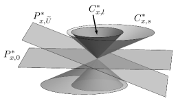
Figure 1. The Characteristic Subset of $T^{*}_{x}\mathcal{M}$

5.2. Characteristic surfaces and the characteristic subset of $T_{x}\mathcal{M}$

A $C^{1}$ surface $S\subset\mathcal{M}$ that is given as a level set of a function $\Phi$ is said to be a characteristic surface if at each point $x\in S,$ the covector $\xi$ with components $\xi_{\nu}=\partial_{\nu}\Phi\ \mbox{for}\ \nu=0,1,2,3,$ is an element of the characteristic subset of $T^{*}_{x}\mathcal{M}.$ It is well-known (consult e.g. [9]) that jump discontinuities in weak solutions can occur across characteristic surfaces, and that characteristic surfaces play a role in determining a domain of influence of a region of spacetime.

There is an alternative characterization of characteristic surfaces in terms of the duals of the sheets $P^{*}_{x,\widetilde{U}},$ $P^{*}_{x,0},$ $C^{*}_{x,s},$ and $C^{*}_{x,l}.$ The notion of duality we refer to is as follows (consult e.g. [9]): To each covector $\xi$ in the characteristic subset of $T_{x}^{*}\mathcal{M}$ there corresponds the null space of $\xi,$ which we denote by $N_{\xi}.$ This 3-dimensional plane is a subset of $T_{x}\mathcal{M}$, the tangent space of $\mathcal{M}$ at $x,$ and is described in coordinates as $N_{\xi}\overset{\mbox{\tiny{def}}}{=}\{X\in T_{x}\mathcal{M}|\xi_{\mu}X^{\mu}=0\}.$ We define the dual to a sheet of the characteristic subset of $T_{x}^{*}\mathcal{M}$ to be the envelope in $T_{x}\mathcal{M}$ generated by the $N_{\xi}$ as $\xi$ varies over the sheet. The characteristic subset of the tangent space at $x$ is defined to be the union of the duals to the sheets (5.1.11) - (5.1.14). A calculation of the envelopes implies that the respective duals to (5.1.11), (5.1.12), (5.1.13), and (5.1.14) are the sets of $X\in T_{x}\mathcal{M}$ such that in our fixed rectangular coordinate system (see Section 2.1),

(5.2.1) $$X =\lambda\widetilde{U}\ \mbox{for some}\ \lambda\in\mathbb{R}$$

(5.2.2) $$\widetilde{h}_{\mu\nu}X^{\mu}X^{\nu} =0$$

(5.2.3) $$\underline{g}{}_{\mu\nu}X^{\mu}X^{\nu} =0$$

(5.2.4) $$X =\lambda(1,0,0,0)\ \mbox{for some}\ \lambda\in\mathbb{R},$$

where

(5.2.5) $$\widetilde{h}_{\mu\nu}\overset{\mbox{\tiny{def}}}{=}\underline{g}{}_{\mu\nu}+(1-\widetilde{\sigma}^{2})\widetilde{U}_{\mu}\widetilde{U}_{\nu}$$

is the acoustical metric, a non-degenerate quadratic form on $T_{x}\mathcal{M}.$ The dual to $P^{*}_{x,\widetilde{U}},$ given by (5.2.1), is the linear span of $\widetilde{U},$ and the dual to the plane $P^{*}_{x,0},$ given by (5.2.4), is the linear span of $(1,0,0,0).$ The dual to $C^{*}_{x,s},$ given by (5.2.2) and labeled as $C_{x,s},$ is the sound cone in $T_{x}\mathcal{M},$ while the dual to $C^{*}_{x,l},$ given by (5.2.3) and labeled as $C_{x,l},$ is the light cone in $T_{x}\mathcal{M}.$ We refer to these subsets of $T_{x}\mathcal{M}$ as the four sheets of the characteristic subset of the $T_{x}\mathcal{M}$ (noting that the degenerate cases (5.2.1) and (5.2.4) are lines rather than “sheets”). See Fig. 2 for the picture in $\mathbb{R}^{1+2},$ where the vertical direction represents positive values of $X^{0}.$

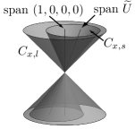
Figure 2. The Characteristic Subset of $T_{x}\mathcal{M}$

It follows from the above description that for each $\xi$ belonging to a fixed sheet of the characteristic subset of $T_{x}^{*}\mathcal{M},$ $N_{\xi}$ is tangent to the corresponding sheet of the characteristic subset of $T_{x}\mathcal{M}.$ Therefore, we may equivalently define a characteristic surface as a $C^{1}$ surface $S$ such that the tangent plane at each of its points $x$ is tangent to any of the four sheets of the characteristic subset of $T_{x}\mathcal{M}.$

Remark 5.2.1.

Note that $C_{x,s}$ lies inside $C_{x,l},$ but $C_{x,l}^{*}$ lies inside $C_{x,s}^{*}.$

5.3. Inner characteristic core, strict hyperbolicity, spacelike surfaces

The inner characteristic core of the cotangent space at $x,$ denoted $\mathcal{I}^{*}_{x},$ is the subset of $T_{x}^{*}\mathcal{M}$ lying strictly inside the innermost sheet $C^{*}_{x,l}.$ $\mathcal{I}^{*}_{x}$ comprises two components, and we refer to the component such that each co-vector $\xi$ belonging to it has $\xi_{0}>0$ as the positive component, denoted by $\mathcal{I}^{*+}_{x}:$

(5.3.1) $$\mathcal{I}^{*+}_{x}\overset{\mbox{\tiny{def}}}{=}\{\xi\in T^{*}_{x}\mathcal{M}|\xi_{\mu}\xi^{\mu}<0\ \mbox{and}\ \xi_{0}>0\}.$$

A co-vector $\xi\in T^{*}_{x}\mathcal{M}$ is said to be hyperbolic for $\mathcal{Q}$ at $x$ iff for any co-vector $\upsilon$ not parallel to $\xi,$ $\mathcal{Q}(x;\lambda\xi+\upsilon)=0$ has real roots in $\lambda,$ where $\mathcal{Q}$ is given in (5.1.7). The set of hyperbolic co-vectors at $x$ is equal to $\mathcal{I}^{*}_{x};$ see Fig. 1. A co-vector $\xi\in T^{*}_{x}\mathcal{M}$ is said to be strictly hyperbolic for $\mathcal{Q}$ at $x$ iff for any co-vector $\upsilon$ not parallel to $\xi,$ $\mathcal{Q}(x;\lambda\xi+\upsilon)=0$ has distinct real roots in $\lambda.$ As mentioned in Section 1, the EOV (and hence the EN_κ system) are (is) not strictly hyperbolic because of the repeated factors in the expression (5.1.7) for $\mathcal{Q}(x;\cdot),$ and because two of the sheets of the characteristic subset of $T^{*}_{x}\mathcal{M}$ intersect.

A $C^{1}$ surface $S\subset\mathcal{M}$ is said to be spacelike (with respect to the light cones $C^{*}_{x,l}$) if at each $x\in S,$ there is a co-vector $\xi$ belonging to $\mathcal{I}^{*}_{x}$ such that the tangent plane to $S$ at $x$ is equal to $N_{\xi}.$ Based on the discussion above, it follows that $S$ is spacelike at $x$ iff the tangent plane to $S$ at $x$ is the null space of a co-vector $\xi$ that is hyperbolic for $\mathcal{Q}$ at $x.$

5.4. Speeds of propagation

It is well-known that for first order symmetric hyperbolic systems, the speeds of propagation are locally governed by the characteristic subsets. For example, in the case that the characteristic subset of $T^{*}_{x}\mathcal{M}$ at each $x$ includes an innermost sheet, the domain of influence of a spacetime point $x^{\prime}$ is contained in the interior of the forward conoid in $\mathcal{M}$ traced out by the set of all curves emanating from $x^{\prime}$ and remaining tangent to the sheets of the characteristic subsets of the $T_{x}\mathcal{M}$ that are dual to the innermost sheets of the characteristic subsets of the $T_{x}^{*}\mathcal{M}$ as the curve parameter varies; consult [21] for a detailed discussion of this fact.

We will later illustrate the occurrence of similar phenomena in the EN_κ system. In this case, the innermost sheet at $x$ is $C^{*}_{x,l},$ the dual of which is $C_{x,l},$ the light cone in $T_{x}\mathcal{M}.$ Therefore, the forward conoid emanating from a spacetime point $x^{\prime}$ is the forward light cone in $\mathcal{M}$ with vertex at $x^{\prime}.$ Thus, one would expect that the fastest speed of propagation in the EN_κ system is the speed of light. This claim is given rigorous meaning below in the uniqueness argument (see Section 7.3.1) which shows, for example, that a solution that is constant in the Euclidean sphere of radius $r$ centered at the point $\mathbf{s}\in\mathbb{R}^{3}$ at $t=0$ remains constant in the Euclidean sphere of radius $r-t$ centered at $\mathbf{s}$ at time $t>0;$ see Remark 7.3.2.

We contrast this to the case of the special-relativistic Euler equations without gravitational interaction, in which there is no Klein-Gordon equation governing the propagation of gravitational waves at the speed of light, and the set $C^{*}_{x,l}$ does not belong to the characteristic subset of $T_{x}^{*}\mathcal{M}.$ The inner sheet at $x$ in this case is $C^{*}_{x,s},$ the dual of which is $C_{x,s},$ the sound cone in $T_{x}\mathcal{M},$ and the methods applied below can be used to show that the fastest local speed of propagation is dictated by the sound cones $C_{x,s}.$ This case is studied in detail in [6] and [7].

5.5. Energy currents

The role of energy currents in the well-posedness proof is to replace the energy principle available for symmetric hyperbolic systems. After providing the definition of an energy current, we illustrate its two key properties, namely that it has the positivity property (5.5.2) below, and that its divergence is lower order in the variation $\dot{\mathbf{V}}.$

5.5.1. The definition of an energy current

Given a variation $\dot{\mathbf{V}}:\mathcal{M}\rightarrow\mathbb{R}^{10}$ and a bgs $\widetilde{\mathbf{V}}:\mathcal{M}\rightarrow\mathbb{R}^{10}$ as defined in Section 4.2, we define the energy current to be the vectorfield $\dot{J}$ with components $\dot{J}^{0},$ $\dot{J}^{j},$ $j=1,2,3,$ in the global rectangular coordinate system given by

$$\dot{J}^{0}\overset{\mbox{\tiny{def}}}{=}\widetilde{U}^{0}\dot{{{\eta}}}^{2} +\frac{\widetilde{U}^{0}}{\widetilde{Q}}\dot{P}^{2}+2\frac{\widetilde{U}_{k}\dot{U}^{k}}{\widetilde{U}^{0}}\dot{P}+(\widetilde{R}+\widetilde{P})\widetilde{U}^{0}\Big{[}\dot{U}^{k}\dot{U}_{k}-\frac{(\widetilde{U}_{k}\dot{U}^{k})^{2}}{(\widetilde{U}^{0})^{2}}\Big{]}$$

$$+\frac{1}{2}\big{[}(\dot{\phi})^{2}+(\dot{\psi}_{0})^{2}+(\dot{\psi}_{1})^{2}+(\dot{\psi}_{2})^{2}+(\dot{\psi}_{3})^{2}\big{]}$$

(5.5.1) $$\dot{J}^{j} \overset{\mbox{\tiny{def}}}{=}\widetilde{U}^{j}\dot{{{\eta}}}^{2}+\frac{\widetilde{U}^{j}}{\widetilde{Q}}\dot{P}^{2}+2\dot{U}^{j}\dot{P}+(\widetilde{R}+\widetilde{P})\widetilde{U}^{j}\Big{[}\dot{U}^{k}\dot{U}_{k}-\frac{(\widetilde{U}_{k}\dot{U}^{k})^{2}}{(\widetilde{U}^{0})^{2}}\Big{]}-\dot{\psi}_{0}\dot{\psi}_{j}.$$

Notation.

In an effort to avoid cluttering the notation, we sometimes suppress the direct dependence of $\dot{J}$ on $\dot{\mathbf{V}}$ and $\widetilde{\mathbf{V}}$ and instead emphasize the indirect dependence of $\dot{J}$ on $(t,\mathbf{s})$ through $\dot{\mathbf{V}}$ and $\widetilde{\mathbf{V}}$ by writing $``\dot{J}(t,\mathbf{s})."$

Terminology: We say that $\dot{J}$ is the energy current for the variation $\dot{\mathbf{V}}$ with coefficients defined by the bgs $\widetilde{\mathbf{V}}.$

Remark 5.5.1.

The theory of hyperbolic PDEs derivable from a Lagrangian, and in particular the derivation of energy currents, is developed by Christodoulou in [6]. For readers interested in studying Christodoulou’s techniques, we remark that the Lagrangian density for (4.1.18) - (4.1.20) (the first 5 scalar equations of the EN_κ system) is expressed in the original variables as $\rho e^{4\phi}.$ The energy current (5.5.1) is the sum of an energy current for the linear Klein-Gordon equation, which supplies the terms involving $(\dot{\phi})^{2}$ and $(\dot{\psi_{\nu}})^{2},$ and an energy current used by Christodoulou in [7] to study the special-relativistic Euler equations without gravitational interaction.

5.5.2. The positive definiteness of $\xi_{\mu}\dot{J}^{\mu}$ for $\widetilde{P}>0$ and $\xi\in\mathcal{I}^{*+}_{x}$

Given an energy current as defined by (5.5.1) and a co-vector $\xi\in T^{*}_{x}\mathcal{M},$ the quantity $\xi_{\mu}\dot{J}^{\mu}$ may be viewed as a quadratic form in the variations $\dot{\mathbf{V}}$ with coefficients defined by the bgs $\widetilde{\mathbf{V}}.$ We emphasize this quadratic dependence on the variations by writing $\xi_{\mu}\dot{J}^{\mu}(\dot{\mathbf{V}},\dot{\mathbf{V}}).$ One of the two key features of the energy current is that $\widetilde{P}>0$ and $\xi\in\mathcal{I}^{*+}_{x}$ together imply that the form $\xi_{\mu}\dot{J}^{\mu}(\dot{\mathbf{V}},\dot{\mathbf{V}})$ is positive definite in $\dot{\mathbf{V}}:$

(5.5.2) $$\xi_{\mu}\dot{J}^{\mu}(\dot{\mathbf{V}},\dot{\mathbf{V}})>0\ \mbox{if}\ \xi\in\{\zeta\in T^{*}_{x}(\mathcal{M})\ |\ \zeta_{\mu}\zeta^{\mu}<0\ \mbox{and}\ \zeta_{0}>0\}\ \mbox{and}\ \dot{\mathbf{V}}\neq\mathbf{0}.$$

A direct verification of this fact can be carried out, for example, by calculating the eigenvalues of the matrix of the quadratic form $\xi_{\mu}\dot{J}^{\mu}(\dot{\mathbf{V}},\dot{\mathbf{V}}).$ The eigenvalues depend on $\xi$ and are positive whenever $\widetilde{P}>0$ and $\xi\in\mathcal{I}^{*+}_{x}.$ As we shall soon see, inequality (5.5.2) will allow us to use the form $\xi_{\mu}\dot{J}^{\mu}(\dot{\mathbf{V}},\dot{\mathbf{V}})$ to estimate the $L^{2}$ norms of the variations, provided that we estimate the bgs $\widetilde{\mathbf{V}}.$

Remark 5.5.2.

Although later in this article we make use of the fact that $\dot{\mathbf{V}}$ is a solution to the EOV, the inequality in (5.5.2) does not rely on this fact; it is an algebraic statement about $\xi_{\mu}\dot{J}^{\mu}(\dot{\mathbf{V}},\dot{\mathbf{V}})$ viewed as a quadratic form on $\mathbb{R}^{10}.$

5.5.3. The divergence of the energy current

If the variations $\dot{\mathbf{V}}$ are solutions of the EOV, then we can compute $\partial_{\mu}\dot{J}^{\mu}$ and use the equations (4.2.1) - (4.2.6) for substitution to eliminate the terms containing the derivatives of $\dot{\mathbf{V}}:$

(5.5.3) $$\begin{split}\partial_{\mu}\dot{J}^{\mu}&=(\partial_{\mu}\widetilde{U}^{\mu})\dot{{{\eta}}}^{2}+\partial_{\mu}\left(\frac{\widetilde{U}^{\mu}}{\widetilde{Q}}\right)\dot{P}^{2}+2\partial_{0}\left(\frac{\widetilde{U}_{k}}{\widetilde{U}^{0}}\right)\dot{U}^{k}\dot{P}\\ &+\partial_{\mu}[(\widetilde{R}+\widetilde{P})\widetilde{U}^{\mu}]\left[\dot{U}^{k}\dot{U}_{k}-\frac{(\widetilde{U}_{k}\dot{U}^{k})^{2}}{(\widetilde{U}^{0})^{2}}\right]-2\widetilde{U}_{k}\dot{U}^{k}(\widetilde{R}+\widetilde{P})\left(\frac{\widetilde{U}^{\mu}}{\widetilde{U}^{0}}\right)\partial_{\mu}\left(\frac{\widetilde{U}_{j}}{\widetilde{U}^{0}}\right)\dot{U}^{j}\\ &+2\dot{{{\eta}}}f+2\frac{\dot{P}g}{\widetilde{Q}}+2\dot{U}_{k}h^{(k)}-2\frac{\widetilde{U}_{j}h^{(j)}\widetilde{U}_{k}\dot{U}^{k}}{(\widetilde{U}^{0})^{2}}-\ {\dot{\psi}}_{0}l^{(0)}\ +\ {\dot{\psi}}_{k}l^{(k)}\ +\ \dot{\phi}l^{(4)}.\end{split}$$

That the right-hand side of (5.5.3) does not contain any derivatives of the variations is the second key property announced at the beginning of Section 5.5.

Remark 5.5.3.

Given a spatial derivative multi-index $\vec{\alpha}$ and an energy current $\dot{J}$ as defined in (5.5.1) such that the variation $\dot{\mathbf{V}}$ is a solution of (4.2.1) - (4.2.10) with inhomogeneous terms $(\mathbf{b},\mathbf{l})$, where $\mathbf{b}$ and $\mathbf{l}$ are defined by (4.2.17) and (4.2.18) respectively, we define the higher-order energy current $\dot{J}_{\vec{\alpha}}$ to be the energy current for the variation $\partial_{\vec{\alpha}}\dot{\mathbf{V}}$ with coefficients defined by the same bgs $\widetilde{\mathbf{V}}.$ The variations $\partial_{\vec{\alpha}}\dot{\mathbf{V}}$ are solutions of (4.2.1) - (4.2.10) with inhomogeneous terms $(\mathbf{b}_{\vec{\alpha}},\partial_{\vec{\alpha}}\mathbf{l}),$ where $\mathbf{b}_{\vec{\alpha}}$ is defined in terms of $\mathbf{b}$ below through (7.2.21). Consequently, the expression for $\partial_{\mu}\dot{J}^{\mu}_{\vec{\alpha}}$ is given by taking the formula (5.5.3) for $\partial_{\mu}\dot{J}^{\mu}$ and making the replacements $\dot{\mathbf{V}}\rightarrow\partial_{\vec{\alpha}}\dot{\mathbf{V}}$ and $(\mathbf{b},\mathbf{l})\rightarrow(\mathbf{b}_{\vec{\alpha}},\partial_{\vec{\alpha}}\mathbf{l}).$

6. Assumptions on the Initial Data

We now describe a class of initial data to which the energy methods for showing well-posedness can be applied. The Cauchy surface we consider is $\{(t,\mathbf{s})\in\mathcal{M}\ |\ t=0\}.$

6.1. An $H^{N}$ perturbation of a quiet fluid

The initial data for the EN_κ system are denoted by $\mathring{\mathbf{V}}=\mathring{\mathbf{V}}(\mathbf{s})\overset{\mbox{\tiny{def}}}{=}(\mathring{{{\eta}}},\mathring{P},\mathring{U}^{1},\cdots,\mathring{\psi}_{3}),$ where $\mathring{\psi}_{j}\overset{\mbox{\tiny{def}}}{=}\partial_{j}\mathring{\phi}$ for $j=1,2,3.$ We assume that the initial data $\mathring{\mathbf{V}}$ for the EN_κ system are constructed from initial data $(\mathring{{{\eta}}},\mathring{p},\mathring{u}^{1},\cdots,\mathring{\psi}_{3})$ in the original state-space variables $({{\eta}},p,u^{1},\cdots,\psi^{3})$ according to the substitutions (4.1.4), (4.1.5), and (4.1.6). Additionally, we assume that outside of the unit ball centered at the origin in the Cauchy surface

(6.1.1) $$\mathring{\mathbf{V}}\equiv\bar{\mathbf{V}}\overset{\mbox{\tiny{def}}}{=}(\bar{{{\eta}}},\bar{P},0,0,0,\bar{\phi},0,0,0,0),$$

where $\bar{\phi}$ is the unique solution to

(6.1.2) $${\kappa}^{2}\bar{\phi}+e^{4\bar{\phi}}\left(\mathscr{R}(\bar{p},\bar{{{\eta}}})-3\bar{p}\right)=0,$$

$\bar{{{\eta}}}$ and $\bar{p}$ are positive constants denoting the initial entropy and pressure of the fluid outside of the unit ball, $\bar{P}\overset{\mbox{\tiny{def}}}{=}e^{4\bar{\phi}}\bar{p},$ and the function $\mathscr{R}$ is defined in (3.3.9). An initial state of this form is a perturbation of an infinitely extended quiet fluid, such that the perturbation is initially contained in the unit ball. Here we need the cosmological constant $\kappa^{2}>0$ in order to ensure that the EN_κ system has non-zero constant solutions of the form $\bar{\mathbf{V}}.$

Because the standard energy methods require that the initial data belong to a Sobolev space of high enough order, we assume that

(6.1.3) $$\|\mathring{{{\eta}}}-\bar{{{\eta}}}\|_{H^{N}}+\|\mathring{p}-\bar{p}\|_{H^{N}}+\|\mathring{u}^{k}\|_{H^{N}}+\|\mathring{\phi}-\bar{\phi}\|_{H^{N+1}}+\|\mathring{\psi}_{0}\|_{H^{N}}<\infty,$$

where $N\in\mathbb{N}$ satisfies

(6.1.4) $$N\geq 3.\$$

Note that (6.1.3) implies that $\|\mathring{\psi}_{j}\|_{H^{N}}<\infty\ (j=1,2,3).$ By Proposition A.2 and Remark A.1, it follows from (6.1.3) that

(6.1.5) $$\|\mathring{\mathbf{V}}\|_{H_{\bar{\mathbf{V}}}^{N}}<\infty.$$

Remark 6.1.1.

It is not necessary to assume that the initial deviation from the constant state has compact support. It is sufficient to consider initial data $\mathring{\mathbf{V}}$ that differ from $\bar{\mathbf{V}}$ by a perturbation belonging to $H^{N},$ such that that $\mathring{\mathbf{V}}(\mathbb{R}^{3})$ is contained in a compact subset of $\mathcal{O},$ where $N$ is given by (6.1.4) and $\mathcal{O}$ is defined in Section 6.2. We make the compactness assumption because it is useful for illustrating the speeds of propagation as discussed in Section 5.4, and because we plan to make use of this setup in future work.

6.2. The admissible subset of state space and the uniform positive definiteness of $\dot{J}^{0}$

In this section we discuss a further positivity restriction that we place on the initial data. We will see in Section 7.2.3 that this positivity condition is propagated for short times during an iterative construction of solutions to the linearized EN_κ system. Since it plays a key role in our future analysis, we discuss here the implications of this positivity restriction regarding the uniform positive definiteness of the energy current, viewed as a quadratic form in the variations.

6.2.1. The definition of the admissible subset of state-space

In order to avoid studying the free boundary problem and in order to avoid singularities in the energy current, we assume that the initial pressure, energy density, and speed of sound are uniformly bounded from below by a positive constant. According to our assumptions (3.3.5) on the equation of state, to satisfy these requirements, it is sufficient to consider initial data for the EN_κ system such that $\mathring{\mathbf{V}}(\mathbb{R}^{3})$ is contained in a compact subset of the following open subset $\mathcal{O}$ of the state-space $\mathbb{R}^{10},$ the admissible subset of state-space:

(6.2.1) $$\mathcal{O}=\{\mathbf{V}\in\mathbb{R}^{10}|{\eta}>0,P>0\}.$$

We therefore assume that $\bar{\mathbf{V}}\in\mathcal{O}_{1}$ and $\mathring{\mathbf{V}}(\mathbb{R}^{3})\subset\mathcal{O}_{1},$ where $\mathcal{O}_{1}$ is a precompact open set with $\bar{\mathcal{O}}_{1}\Subset\mathcal{O}.$ We then fix a precompact open subset $\mathcal{O}_{2}$ with convex closure satisfying $\bar{\mathcal{O}}_{1}\Subset\mathcal{O}_{2}\subset\bar{\mathcal{O}}_{2}\Subset\mathcal{O};$ our goal is to show the existence of a solution that remains in $\bar{\mathcal{O}}_{2}$ for short times.

6.2.2. The uniform positive definiteness of $\dot{J}^{0}$

Most of the technical exposition below is devoted to obtaining control over $\|\dot{\mathbf{V}}(t)\|_{H^{N}},$ where $\dot{\mathbf{V}}$ is a solution to the EOV defined by a bgs $\widetilde{\mathbf{V}}.$ Instead of trying to estimate $\|\dot{\mathbf{V}}(t)\|_{L^{2}}$ directly, it is advantageous to estimate $\|\dot{J}^{0}(t)\|_{L^{1}},$ where $\dot{J}$ is an energy current for $\dot{\mathbf{V}}$ with coefficients defined by the bgs $\widetilde{\mathbf{V}},$ since the divergence of $\dot{J}$ is lower order in $\dot{\mathbf{V}}.$ A similar remark applies to estimating $\|\partial_{\vec{\alpha}}\dot{\mathbf{V}}\|_{L^{2}}$ using higher-order energy currents $\dot{J}_{\vec{\alpha}}.$ We shall see that $\|\dot{J}^{0}(t)\|_{L^{1}}$ can be used to estimate $\|\dot{\mathbf{V}}(t)\|^{2}_{L^{2}}$ from above and below provided that $\dot{J}^{0}$ is uniformly positive definite independent of the bgs $\widetilde{\mathbf{V}}.$ More precisely, we claim that there exists a $C_{\bar{\mathcal{O}}_{2}}$ with $0<C_{\bar{\mathcal{O}}_{2}}<1$ such that for any variation $\dot{\mathbf{V}}$ and any bgs $\widetilde{\mathbf{V}}$ contained in $\bar{\mathcal{O}}_{2},$ we have

(6.2.2) $$C_{\bar{\mathcal{O}}_{2}}|\dot{\mathbf{V}}|^{2}\leq\dot{J}^{0}(\dot{\mathbf{V}},\dot{\mathbf{V}})\leq\frac{1}{C_{\bar{\mathcal{O}}_{2}}}|\dot{\mathbf{V}}|^{2}.$$

To prove (6.2.2), recall that $\dot{J}$ is defined by (5.5.1) and note that $(1,0,0,0)\in\mathcal{I}^{*+}_{x}$ by (5.5.2). The uniform continuity of $\dot{J}$ (which we momentarily view as a function of $(\widetilde{\mathbf{V}},\dot{\mathbf{V}})$) on the compact set $\bar{\mathcal{O}}_{2}\times\{|\dot{\mathbf{V}}|=1\}$ implies that there exists a $C_{\bar{\mathcal{O}}_{2}}$ with $0<C_{\bar{\mathcal{O}}_{2}}<1$ such that (6.2.2) holds whenever $\widetilde{\mathbf{V}}(t,\mathbf{s})\in\bar{\mathcal{O}}_{2}$ and $|\dot{\mathbf{V}}|=1.$ Since the inequalities in (6.2.2) are invariant under any rescaling of $\dot{\mathbf{V}},$ it follows that we may remove the restriction $|\dot{\mathbf{V}}|=1.$

7. The Well-Posedness Theorems

In this section, we state and indicate how to prove our two main theorems. We have separated the proof of well-posedness into two theorems since the techniques used in proving each are different. Statements of the technical estimates involving the Sobolev-Moser calculus have been placed in the Appendix so as to not interrupt the flow of the main argument.

Theorem 1.

(Local Existence and Uniqueness) Let $\mathring{\mathbf{V}}(\mathbf{s})$ be initial data for the EN_κ system (4.1.18) - (4.1.26) that are subject to the conditions described in Section 6. Then there exists a $T>0$ such that (4.1.18) - (4.1.26) has a unique classical solution $\mathbf{V}(t,\mathbf{s})$ on $[0,T]\times\mathbb{R}^{3}$ satisfying $\mathbf{V}(0,\mathbf{s})=\mathring{\mathbf{V}}(\mathbf{s}).$ The solution is of the form $\mathbf{V}=({{\eta}},P,U^{1},U^{2},U^{3},\phi,\partial_{0}\phi,\partial_{1}\phi,\partial_{2}\phi,\partial_{3}\phi)$ and satisfies
$\mathbf{V}([0,T]\times\mathbb{R}^{3})\subset\bar{\mathcal{O}}_{2}.$ Furthermore,
$\mathbf{V}\in C_{b}^{1}([0,T]\times\mathbb{R}^{3})\cap C^{0}([0,T],H_{\bar{\mathbf{V}}}^{N})\cap C^{1}([0,T],H_{\bar{\mathbf{V}}}^{N-1}),$ and consequently
$\phi\in C_{b}^{2}([0,T]\times\mathbb{R}^{3})\cap C^{0}([0,T],H_{\bar{\phi}}^{N+1})\cap C^{1}([0,T],H_{\bar{\phi}}^{N})\cap C^{2}([0,T],H_{\bar{\phi}}^{N-1}).$

Proof.

As discussed in Section 7.1, our abbreviated proof of Theorem 1 is located in Section 7.2. ∎

Remark 7.0.1.

In the discussion below, we sometimes denote the solution from Theorem 1 by $\mathbf{V}_{sol}$ for clarity.

Corollary 7.0.1.

The interval of existence $[0,T]$ supplied by the Theorem 1 depends only on the set $\bar{\mathcal{O}}_{2}$ from Section 6, $\|{{}^{(0)}\mathring{\mathbf{V}}}\|_{H_{\bar{\mathbf{V}}}^{N+1}},$ and the constant $\Lambda$ chosen in (7.2.7) - (7.2.9) below. Here, ${{}^{(0)}\mathring{\mathbf{V}}}$ denotes the mollified initial data as described in Section 7.2. Furthermore, the set $\bar{\mathcal{O}}_{2},$ the mollified initial data ${{}^{(0)}\mathring{\mathbf{V}}},$ and constant $\Lambda$ can be chosen to be independent of all initial data varying in a small $H^{N}$ neighborhood of $\mathring{\mathbf{V}}.$ Therefore, if we define $B_{y}(\mathring{\mathbf{V}})\overset{\mbox{\tiny{def}}}{=}\{\mathring{\widetilde{\mathbf{V}}}\in H_{\bar{\mathbf{V}}}^{N}\ |\ \|\mathring{\widetilde{\mathbf{V}}}-\mathring{\mathbf{V}}\|_{H^{N}}<y\},$ then there exist $\delta>0$ and $T^{\prime}>0$ (depending on $\mathring{\mathbf{V}}$) such that any initial data $\mathring{\widetilde{\mathbf{V}}}$ belonging to $B_{\delta}(\mathring{\mathbf{V}})$ launch a unique classical solution $\widetilde{\mathbf{V}}$ that exists on the common time interval $[0,T^{\prime}]$ and that has the property $\widetilde{\mathbf{V}}([0,T^{\prime}]\times\mathbb{R}^{3})\subset\bar{\mathcal{O}}_{2}.$

Proof.

The corollary follows from the proof of Theorem 1. See in particular Remark 7.2.1 and Remark 7.2.2 below. ∎

Corollary 7.0.2.

The norms $\mid\mid\mid\mathbf{V}\mid\mid\mid_{H_{\bar{\mathbf{V}}}^{N},T}$ and $\mid\mid\mid\partial_{t}\mathbf{V}\mid\mid\mid_{H^{N-1},T}$ of the solution from Theorem 1 depend only $\bar{\mathcal{O}}_{2},$ $\|{{}^{(0)}\mathring{\mathbf{V}}}\|_{H_{\bar{\mathbf{V}}}^{N+1}},$ and $\Lambda.$ Furthermore, there exists a $K>0$ such that any initial data $\mathring{\widetilde{\mathbf{V}}}$ belonging to the set $B_{\delta}(\mathring{\mathbf{V}})$ defined in Corollary 7.0.1 launch a unique solution $\widetilde{\mathbf{V}}$ that satisfies the uniform bound

(7.0.1) $$\mid\mid\mid\widetilde{\mathbf{V}}\mid\mid\mid_{H_{\bar{\mathbf{V}}}^{N},T^{\prime}},\mid\mid\mid\partial_{t}\widetilde{\mathbf{V}}\mid\mid\mid_{H^{N-1},T^{\prime}}<K(N,\bar{\mathcal{O}}_{2},\|{{}^{(0)}\mathring{\mathbf{V}}}\|_{H_{\bar{\mathbf{V}}}^{N+1}},\Lambda,\delta),$$

where $T$ and $T^{\prime}$ are as in Corollary 7.0.1.

Proof.

The estimates for $\mid\mid\mid\mathbf{V}\mid\mid\mid_{H_{\bar{\mathbf{V}}}^{N},T}$ and $\mid\mid\mid\widetilde{\mathbf{V}}\mid\mid\mid_{H_{\bar{\mathbf{V}}}^{N},T^{\prime}}$ follow from Corollary 7.0.1, Proposition 7.2.1, and the fact that the sequence of iterates $\{{{}^{(m)}\mathring{\mathbf{V}}}(t)\}$ constructed below converges strongly in $L_{\bar{\mathbf{V}}}^{2}$ and weakly in $H_{\bar{\mathbf{V}}}^{N}$ to $\mathbf{V}(t);$ consult [22] for the missing details. We then use the EN_κ equations to solve for the time derivatives together with Proposition A.2 and Remark A.1 to obtain the estimates for
$\mid\mid\mid\partial_{t}\mathbf{V}\mid\mid\mid_{H^{N-1},T}$ and $\mid\mid\mid\partial_{t}\widetilde{\mathbf{V}}\mid\mid\mid_{H^{N-1},T^{\prime}}.$ ∎

Theorem 2.

(Continuous Dependence on Initial Data) Let $\mathring{\mathbf{V}}(\mathbf{s})$ be initial data for the EN_κ system (4.1.18) - (4.1.26) that are subject to the conditions described in Section 6, and let $\mathbf{V}$ be the solution existing on the time interval $[0,T]$ furnished by Theorem 1. Let $B_{\delta}(\mathring{\mathbf{V}})$ be as in Corollary 7.0.1. Let $\{\mathring{\mathbf{V}}^{m}\}\subset B_{\delta}$ be a sequence of initial data with $\lim_{m\to\infty}\|\mathring{\mathbf{V}}^{m}-\mathring{\mathbf{V}}\|_{H^{N}}=0,$ and let $\mathbf{V}^{m}$ denote the solution to (4.1.18) - (4.1.26) launched by $\mathring{\mathbf{V}}^{m}.$ Then for all large $m,$ the solutions $\mathbf{V}^{m}$ exist on $[0,T],$ and $\lim_{m\to\infty}\mid\mid\mid\mathbf{V}^{m}-\mathbf{V}\mid\mid\mid_{H^{N},T}=0.$

Proof.

Our proof of Theorem 2 is located in Section 7.4. ∎

Remark 7.0.2.

It is unknown to the author whether or not the continuity statement from Theorem 2 can be strengthened to one of Lipschitz continuity or Hölder continuity. However, using Burger’s equation $\partial_{t}u+u\partial_{x}u=0,$ Kato [18] provides a counterexample in which the map from the initial data $u_{0}\in H^{a}(\mathbb{R})$ to the solution $u(t)\in C([0,T],H^{a})$ is not Hölder continuous with any positive exponent; such a counterexample is explicitly constructed for $a\geq 2.$ On the other hand, inequality (7.3.27) below shows that for the EN_κ system, the map from the initial data to the solution is a Lipschitz-continuous map from $H_{\bar{\mathbf{V}}}^{N}$ into $C([0,T],H_{\bar{\mathbf{V}}}^{N-1}).$

7.1. A discussion of the structure of the proof of the theorems

We prove local existence by following a standard method described in detail in Majda’s book [22]: we construct a sequence of iterates $\{{{}^{(m)}\mathbf{V}}(t,\mathbf{s})\}$ that converges to the solution $\mathbf{V}_{sol}(t,\mathbf{s}).$ To construct the iterates, we first define a sequence of $C^{\infty}$ initial data $\{{{}^{(m)}\mathring{\mathbf{V}}}\}$ such that ${{}^{(m)}\mathring{\mathbf{V}}}(\mathbb{R}^{3})\Subset\mathcal{O}_{2}$ and $\lim_{m\to\infty}\mid\mid{{}^{(m)}\mathring{\mathbf{V}}}-\mathring{\mathbf{V}}\mid\mid_{H^{N}}=0.$ The advantage of smoothing the data is that all of the iterates are $C^{\infty},$ thus allowing us to work with classical derivatives during the approximation process. Then beginning with ${{}^{(0)}\mathbf{V}}(t,\mathbf{s})\overset{\mbox{\tiny{def}}}{=}{{}^{(0)}\mathring{\mathbf{V}}}(\mathbf{s}),$ we inductively define ${{}^{(m+1)}\mathbf{V}}(t,\mathbf{s})$ as the unique solution to the linearization of the EN_κ system around ${{}^{(m)}\mathbf{V}}(t,\mathbf{s})$ with initial data ${{}^{(m+1)}\mathbf{V}}(0,\mathbf{s})={{}^{(m+1)}\mathring{\mathbf{V}}}(\mathbf{s}).$ As a consequence of the theory of linear PDEs (consult [9]), each iterate ${{}^{(m)}\mathbf{V}}$ is known to possess a classical solution on a strip $[0,T_{m}]\times\mathbb{R}^{3},$ on which it satisfies, for every real number $N^{\prime},$ ${{}^{(m)}\mathbf{V}}\in C^{0}([0,T_{m}],H_{\bar{\mathbf{V}}}^{N^{\prime}}).$ Here, $T_{m}$ is any real number such that ${{}^{(m-1)}\mathbf{V}}([0,T_{m}]\times\mathbb{R}^{3})\subset\bar{\mathcal{O}}_{2},$ which ensures that the sequence of proper energy densities is bounded from below by a uniform constant and therefore precludes singularities in energy the currents we use during the linearization process.

In order for the limiting function $\mathbf{V}_{sol}$ to be defined on a strip, it is obviously necessary that we show that the sequence of time values $\{T_{m}\}$ can be bounded from below by a positive constant $T_{*}.$ To this end, we examine the EOV satisfied by ${{}^{(m)}\mathbf{V}}-{{}^{(0)}\mathring{\mathbf{V}}}$ and its partial derivatives, and we control the growth in $T_{*}$ of $\mid\mid\mid{{}^{(m)}\mathbf{V}}-{{}^{(0)}\mathring{\mathbf{V}}}\mid\mid\mid_{H^{N},T_{*}}$ uniformly in $m$ using energy currents. According to the above paragraph and the Sobolev embedding result $H^{2}(\mathbb{R}^{3})\subset C^{0}_{b}(\mathbb{R}^{3}),$ it follows that if $\mid\mid\mid{{}^{(m)}\mathbf{V}}-{{}^{(0)}\mathring{\mathbf{V}}}\mid\mid\mid_{H^{N},T_{*}}$ is small enough, uniformly in $m,$ then $T_{*}$ may be selected as a uniform lower bound on the $T_{m}.$ Our detailed proof of the control of the terms $\mid\mid\mid{{}^{(m)}\mathbf{V}}-{{}^{(0)}\mathring{\mathbf{V}}}\mid\mid\mid_{H^{N},T_{*}}$ is given in Proposition 7.2.1 below and uses the Sobolev-Moser calculus inequalities, which are refined versions of the fact that for $N^{\prime}>\frac{3}{2},$ $H^{N^{\prime}}(\mathbb{R}^{3})$ is a Banach algebra. Their purpose is to control the $L^{2}$ norms of terms of a product form, based on known Sobolev regularity of each factor in the product. We state the relevant Sobolev-Moser estimates in the Appendix and give references for readers interested in the proofs.

Our proof of Proposition 7.2.1 illustrates the relevant techniques for obtaining Sobolev estimates from the method of energy currents. Instead of completing the existence proof, which requires arguments similar to the ones used in proving this proposition, we refer the reader to Majda’s local existence proof for symmetric hyperbolic systems [22]; the only necessary modification to Majda’s proof is to use the method of energy currents in place of the energy principle for symmetric hyperbolic systems.

In Section 7.3.1 we show uniqueness and $H^{N-1}-$Lipschitz-continuous dependence on the initial data. The methods used in this argument are similar to the methods used to prove Proposition 7.2.1, so we provide fewer details. We consider the EOV satisfied by the difference of two solutions $\mathbf{V}$ and $\widetilde{\mathbf{V}}$ to the EN_κ system, and then use an appropriately defined energy current to bound the growth of $\mid\mid\mid\mathbf{V}-\widetilde{\mathbf{V}}\mid\mid\mid_{H^{N-1},T}$ by a constant times exponential growth in $T.$ We show that the constant depends on the initial data and is bounded from above by another constant times $\|\mathbf{V}(0)-\widetilde{\mathbf{V}}(0)\|_{H^{N-1}},$ thus implying uniqueness and $H^{N-1}-$Lipschitz-continuous dependence on the initial data. Our abbreviated proof of Theorem 1 is complete at the end of this section.

Our proof of Theorem 2 requires some machinery from the theory of evolution equations in a Banach space. The basic method is due to Kato [18], and most of the technical results we use in this section are merely quoted from his papers. We find it worthwhile to prove Theorem 2 because aside from Kato’s work, we have had difficulty locating this result in the literature.

7.2. An abbreviated proof of Theorem 1

As described in Section 7.1, we produce a sequence of iterates $\{{{}^{(m)}\mathbf{V}}(t,\mathbf{s})\}$ that converges to the solution $\mathbf{V}_{sol}(t,\mathbf{s}).$

7.2.1. Smoothing the initial data

We begin by smoothing the initial data $\mathring{\mathbf{V}},$ which we assume are of the form described in Section 6, so that we can work with classical derivatives. Let $\Psi(\mathbf{s})$ be a Friedrich’s mollifier; i.e. $\Psi\in C_{c}^{\infty}(\mathbb{R}^{3}),\ \mbox{supp}(\Psi)\subset\{\mathbf{s}|\ |\mathbf{s}|\leq 1\},\Psi\geq 0,$ and $\int\Psi\ d^{3}\mathbf{s}=1.$ For $\epsilon>0,$ we set $\Psi_{\epsilon}(\mathbf{s})\overset{\mbox{\tiny{def}}}{=}{\epsilon}^{-3}\Psi(\frac{\mathbf{s}}{\epsilon})$ and define $\Psi_{\epsilon}\mathring{\mathbf{V}}\in C^{\infty}(\mathbb{R}^{3})$ by

(7.2.1) $$\Psi_{\epsilon}\mathring{\mathbf{V}}(\mathbf{s})\overset{\mbox{\tiny{def}}}{=}\int_{\mathbb{R}^{3}}\Psi_{\epsilon}(\mathbf{s}-\mathbf{s}^{\prime})\mathring{\mathbf{V}}(\mathbf{s}^{\prime})\,d^{3}\mathbf{s^{\prime}}.$$

The following properties of such a mollification are well-known:

(7.2.2) $$\underset{\epsilon\rightarrow 0^{+}}{\lim}\|\Psi_{\epsilon}\mathring{\mathbf{V}}-\mathring{\mathbf{V}}\|_{H^{N}} =0$$

(7.2.3) $$\exists\{\epsilon_{0}>0\land C(\mathring{\mathbf{V}})>0\}\owns 0<\epsilon<\epsilon_{0} \Rightarrow\|\Psi_{\epsilon}\mathring{\mathbf{V}}-\mathring{\mathbf{V}}\|_{L^{2}}\leq\epsilon C(\mathring{\mathbf{V}})\|\mathring{\mathbf{V}}\|_{H^{1}}.$$

We will choose below an $\epsilon_{0}$ that is at least as small as the one in (7.2.3). Once chosen, for a given $m\in\mathbb{N},$ we define

(7.2.4) $$\epsilon_{m} \overset{\mbox{\tiny{def}}}{=}2^{-m}\epsilon_{0}$$

(7.2.5) $${{}^{(m)}\mathring{\mathbf{V}}} \overset{\mbox{\tiny{def}}}{=}\Psi_{\epsilon_{m}}\mathring{\mathbf{V}}$$

(7.2.6) $${{}^{(m)}\mathring{\mathbf{W}}} \overset{\mbox{\tiny{def}}}{=}\Psi_{\epsilon_{m}}\mathring{\mathbf{W}},$$

where $\mathring{\mathbf{W}}$ denotes the first 5 components of $\mathring{\mathbf{V}}.$

By Sobolev embedding, by the assumptions on the initial data $\mathring{\mathbf{V}}$, and by the mollification properties above, $\exists\{\Lambda>0\land\epsilon_{0}>0\}$ (at least as small as the $\epsilon_{0}$ in (7.2.3)) such that

(7.2.7) $$\|\mathring{\mathbf{V}}-{{}^{(0)}\mathring{\mathbf{V}}}\|_{H^{N}} \leq C_{\bar{\mathcal{O}}_{2}}\frac{\Lambda}{4}$$

(7.2.8) $$\|\mathbf{V}-{{}^{(0)}\mathring{\mathbf{V}}}\|_{H^{N}} \leq\Lambda\Rightarrow\mathbf{V}(\mathbb{R}^{3})\subset\bar{\mathcal{O}}_{2}$$

(7.2.9) $$\|{{}^{(m)}\mathring{\mathbf{V}}}-{{}^{(0)}\mathring{\mathbf{V}}}\|_{H^{N}} \leq C_{\bar{\mathcal{O}}_{2}}\frac{\Lambda}{2}\ \mbox{holds for}\ m\geq 0,$$

where $C_{\bar{\mathcal{O}}_{2}}$ is defined in (6.2.2).

Remark 7.2.1.

It is a standard result that if $\epsilon>0$ and $N^{\prime}$ is any real number, then $\Psi_{\epsilon}\mathring{\mathbf{V}}\in H_{\bar{\mathbf{V}}}^{N^{\prime}}(\mathbb{R}^{3}).$ We will make use of this remark below, for in the local existence proof, we will need to differentiate the equations (7.2.15) - (7.2.20) $N$ times and utilize Sobolev estimates; since several terms from these undifferentiated equations already contain one derivative of the smoothed initial data, our estimates will involve $\|{{}^{(0)}\mathring{\mathbf{V}}}\|_{H_{\bar{\mathbf{V}}}^{N+1}}.$ See e.g. (7.3.6) and (7.3.9).

Remark 7.2.2.

If we are considering initial data $\mathring{\widetilde{\mathbf{V}}}$ in a small enough $H^{N}$ neighborhood $\mathcal{N}$ of the initial data $\mathring{\mathbf{V}},$ we can use a fixed smoothed function ${{}^{(0)}\mathring{\mathbf{V}}}$ in place of each ${{}^{(0)}\mathring{\widetilde{\mathbf{V}}}}$ in Proposition 7.2.1 below, and choose $\Lambda$ to be uniform over the neighborhood. For what then enters into the proof of local existence for the initial data $\mathring{\widetilde{\mathbf{V}}}$ are the quantities $\|{{}^{(0)}\mathring{\mathbf{V}}}\|_{H_{\bar{\mathbf{V}}}^{N+1}}$ and $\|{{}^{(m)}\mathring{\widetilde{\mathbf{V}}}}-{{}^{(0)}\mathring{\mathbf{V}}}\|_{H^{N}},$ and the latter quantity is easily controlled by the inequality

(7.2.10) $$\|{{}^{(m)}\mathring{\widetilde{\mathbf{V}}}}-{{}^{(0)}\mathring{\mathbf{V}}}\|_{H^{N}}\leq\|{{}^{(m)}\mathring{\widetilde{\mathbf{V}}}}-\mathring{\widetilde{\mathbf{V}}}\|_{H^{N}}+\|\mathring{\widetilde{\mathbf{V}}}-\mathring{\mathbf{V}}\|_{H^{N}}+\|\mathring{\mathbf{V}}-{{}^{(0)}\mathring{\mathbf{V}}}\|_{H^{N}};$$

once we fix an appropriately chosen smoothed function ${{}^{(0)}\mathring{\mathbf{V}}}$ and a corresponding $\Lambda$ satisfying (7.2.7) and (7.2.8), we may independently adjust the mollification of each $\mathring{\widetilde{\mathbf{V}}}$ belonging to $\mathcal{N}$ so that the right-hand side of (7.2.10) is $\leq C_{\bar{\mathcal{O}}_{2}}\Lambda/2$ for $m\geq 0.$ This estimate would then enter into our proof in inequality (7.2.3). We also note that this remark is relevant for Corollary 7.0.1 above.

7.2.2. Defining the iterates

Consider the iteration scheme described in Section 7.1. The components of the iterates are denoted by ${{}^{(m)}\mathbf{V}}=\left({{}^{(m)}{\eta}},{{}^{(m)}P},\cdots,{{}^{(m)}\psi_{3}}\right),$ and we use the notation ${{}^{(m)}\mathbf{W}}$ to denote the first five components of ${{}^{(m)}\mathbf{V}}.$ Linear existence theory implies that each iterate ${{}^{(m+1)}\mathbf{V}}$ is a well-defined, smooth function with $\|{{}^{(m+1)}\mathbf{V}}(t)-{{}^{(0)}\mathring{\mathbf{V}}}\|_{H^{N}}<\infty$ for $0\leq t\leq T_{m}.$ Here, by (7.2.8), $[0,T_{m}]$ is any time interval for which $\mid\mid\mid{{}^{(m)}\mathbf{V}}-{{}^{(0)}\mathring{\mathbf{V}}}\mid\mid\mid_{H^{N},T_{m}}\leq\Lambda$ holds.

7.2.3. The uniform time estimate

As discussed in Section 7.1, we show the existence of a fixed $T_{*}>0$ such that $\mid\mid\mid{{}^{(m)}\mathbf{V}}-{{}^{(0)}\mathring{\mathbf{V}}}\mid\mid\mid_{H^{N},T_{*}}\leq\Lambda$ for $m\in\mathbb{N},$ thus ensuring that each iterate is defined for a uniform amount of time and remains inside of $\bar{\mathcal{O}}_{2}.$ We state a slightly stronger version of this result as a proposition:

Proposition 7.2.1.

Let $\Lambda$ denote the constant defined in (7.2.7) - (7.2.9). Then there exist $T_{*}>0$ and $L>0$ such that each of the iterates ${{}^{(m)}\mathbf{V}}(t,\mathbf{s})$ satisfies

(7.2.11a) $$\mid\mid\mid{{}^{(m)}\mathbf{V}}-{{}^{(0)}\mathring{\mathbf{V}}}\mid\mid\mid_{H^{N},T_{*}}\leq\Lambda$$

(7.2.11b) $$\mid\mid\mid\partial_{t}\big{(}{{}^{(m)}\mathbf{V}}\big{)}\mid\mid\mid_{H^{N-1},T_{*}}\leq L.$$

Proof. We proceed in our proof of Proposition 7.2.1 by induction on $m,$ noting that ${{}^{(0)}\mathbf{V}(t,\mathbf{s})}\overset{\mbox{\tiny{def}}}{=}{{}^{(0)}\mathring{\mathbf{V}}}(\mathbf{s})$ satisfies (7.2.11a) and (7.2.11b) with any $T_{*}>0$ and any positive number $L$. We thus assume that ${}^{(m)}\mathbf{V}$ satisfies (7.2.11a) and (7.2.11b) without first specifying the values of $T_{*}$ or $L.$ At the end of the proof, we will show that we can choose such a $T_{*}$ and an $L,$ both independent of $m,$ such that energy estimates imply the inductive step. To obtain the estimates stated in the proposition, it is convenient to work not with the iterates themselves, but with the difference between the iterate and the smoothed initial value. Thus, referring to the notation defined in (7.2.5) and (7.2.6) , for each $m\in\mathbb{N}$ we define

(7.2.12) $$\dot{\mathbf{V}}(t,\mathbf{s}) \overset{\mbox{\tiny{def}}}{=}{{}^{(m+1)}\mathbf{V}}(t,\mathbf{s})-{{}^{(0)}\mathring{\mathbf{V}}}(\mathbf{s})$$

(7.2.13) $$\dot{\mathbf{W}}(t,\mathbf{s}) \overset{\mbox{\tiny{def}}}{=}{{}^{(m+1)}\mathbf{W}}(t,\mathbf{s})-{{}^{(0)}\mathring{\mathbf{W}}}(\mathbf{s})$$

(7.2.14) $$\widetilde{\mathbf{V}} \overset{\mbox{\tiny{def}}}{=}{{}^{(m)}\mathbf{V}}.$$

We have used the notation $\dot{\mathbf{V}}$ and $\widetilde{\mathbf{V}}$ suggestively: it follows from the the definition of the iterates, definition (7.2.12), and definition (7.2.14) that $\dot{\mathbf{V}}$ is a solution to the EOV (4.2.1) - (4.2.10) defined by the bgs $\widetilde{\mathbf{V}}$ with initial data $\dot{\mathbf{V}}(0,\mathbf{s})={{}^{(m+1)}\mathring{\mathbf{V}}}(\mathbf{s})-{{}^{(0)}\mathring{\mathbf{V}}}(\mathbf{s}).$ Our notation (7.2.12) - (7.2.14) is therefore consistent with our notation for the EOV introduced in Section 4.2. Recalling also the notation (4.2.17) and (4.2.18) introduced in Section 4.2, the inhomogeneous terms in the EOV satisfied by $\dot{\mathbf{V}}$ are given by $(\mathbf{b},\mathbf{l})=(f,g,\cdots,l^{(4)}),$ where for $j=1,2,3,$

(7.2.15) $$f =-\widetilde{U}^{k}\partial_{k}[{{}^{(0)}\mathring{{{\eta}}}}]$$

(7.2.16) $$g =-\widetilde{U}^{k}\partial_{k}[{{}^{(0)}\mathring{P}}]\ -\ \widetilde{Q}\partial_{k}[{{}^{(0)}\mathring{U}^{k}}]\ +\ (4\widetilde{P}-3\widetilde{Q})\widetilde{U}^{\mu}\widetilde{\psi}_{\mu}$$

(7.2.17) $$h^{(j)} =-(\widetilde{R}+\widetilde{P})\widetilde{U}^{k}\partial_{k}[{{}^{(0)}\mathring{U}^{j}}]\ -\widetilde{\Pi}^{kj}\partial_{k}[{{}^{(0)}\mathring{P}}]+(3\widetilde{P}-\widetilde{R})\widetilde{\Pi}^{\mu j}\widetilde{\psi}_{\mu}$$

(7.2.18) $$l^{(0)} =\kappa^{2}\widetilde{\phi}+\widetilde{R}-3\widetilde{P}-\partial^{k}[{{}^{(0)}\mathring{\psi}_{k}}]$$

(7.2.19) $$l^{(j)} =\partial^{j}[{{}^{(0)}\mathring{\psi}_{0}}]$$

(7.2.20) $$l^{(4)} =\widetilde{\psi}_{0}.$$

As explained in Section 4.2, for each spatial derivative multi-index $\vec{\alpha}$ with
$0\leq|\vec{\alpha}|\leq N,$ we may differentiate the EOV with inhomogeneous terms $(\mathbf{b},\mathbf{l})$ to which $\dot{\mathbf{V}}$ is a solution, obtaining that $\partial_{\vec{\alpha}}\dot{\mathbf{V}}$ is also a solution to the EOV defined by the same bgs $\widetilde{\mathbf{V}}$ with inhomogeneous terms $(\mathbf{b}_{\vec{\alpha}},\partial_{\vec{\alpha}}\mathbf{l}).$ The inhomogeneous terms $\mathbf{b}_{\vec{\alpha}}$ are given by

(7.2.21) $$\mathbf{b}_{\vec{\alpha}}\overset{\mbox{\tiny{def}}}{=}A^{0}\partial_{\vec{\alpha}}\left((A^{0})^{-1}\mathbf{b}\right)+\mathbf{k}_{\vec{\alpha}},$$

where

(7.2.22) $$\mathbf{k}_{\vec{\alpha}}\overset{\mbox{\tiny{def}}}{=}A^{0}\left[(A^{0})^{-1}A^{k}\partial_{k}(\partial_{\vec{\alpha}}\dot{\mathbf{W}})-\partial_{\vec{\alpha}}\left((A^{0})^{-1}A^{k}\partial_{k}\dot{\mathbf{W}}\right)\right]$$

for $0\leq|\vec{\alpha}|\leq N.$ Note that we have suppressed the dependence of the $A^{\nu}(\cdot)$ on $\widetilde{\mathbf{V}}.$

As discussed in Section 6.2.2, we will use energy currents to control $\mid\mid\mid\dot{\mathbf{V}}\mid\mid\mid_{H^{N},T}.$ We state here as a lemma an important differential inequality that allows us to proceed with our desired Sobolev estimates. Its proof is based on the key properties of energy currents described in Section 5.5 and the divergence theorem.

Lemma 7.2.2.

(See Fig. 3) Suppose $r\geq T>0.$ For $0\leq t\leq T,$ let
$\Sigma_{t,r-t}\overset{\mbox{\tiny{def}}}{=}\{x\in\mathcal{M}|x^{0}=t,x^{k}x_{k}\leq r-t\}$ denote the Euclidean sphere of radius $r-t$ centered at $(t,0,0,0)$ in the flat hypersurface $\{x^{0}=t\},$ and let
$M_{t,r}\overset{\mbox{\tiny{def}}}{=}\{x\in\mathcal{M}|0\leq x^{0}\leq t,x^{k}x_{k}=r-x^{0}\}$ denote the mantle of the past directed, truncated light cone with lower base $\Sigma_{0,r}$ and upper base $\Sigma_{t,r-t}.$ Let $\dot{\mathbf{V}}$ be a solution to the EOV (4.2.1) - (4.2.10) defined by the bgs $\widetilde{\mathbf{V}},$ and assume that
$\widetilde{\mathbf{V}}([0,T]\times\mathbb{R}^{3})\subset\bar{\mathcal{O}}_{2}.$ Let $\dot{J}$ be the energy current (5.5.1) for the variation $\dot{\mathbf{V}}$ defined by the bgs $\widetilde{\mathbf{V}},$ and define $\mathscr{E}(t;r)\overset{\mbox{\tiny{def}}}{=}\Big{(}\underset{\Sigma_{t,r-t}}{\int}\dot{J}^{0}(t,\mathbf{s})\,d^{3}\mathbf{s}\Big{)}^{1/2}.$ Then

(7.2.23) $$2\mathscr{E}(t;r)\frac{d}{dt}\mathscr{E}(t;r)\leq\underset{\Sigma_{t,r-t}}{\int}\partial_{\mu}\dot{J}^{\mu}(t,\mathbf{s})\,d^{3}\mathbf{s}.$$

Remark 7.2.3.

We note that our use of $t$ in the statement of Lemma 7.2.2 as a constant value taken on by the generic spacetime coordinate $x^{0}$ is inconsistent with our usual notational convention for spacetime points defined in Section 2.1, in which $t$ and $x_{0}$ are both used in the same manner as generic coordinate variables.

Proof.

By the divergence theorem, we have that

$$\mathscr{E}^{2}(t;r)=\underset{\Sigma_{t,r-t}}{\int}\dot{J}^{0}(t,\mathbf{s})\,d^{3}\mathbf{s}=\underset{\Sigma_{0,r}}{\int}\dot{J}^{0}(0,\mathbf{s})\,d^{3}\mathbf{s}\$$

(7.2.24) $$-\ \underset{M_{t,r}}{\int}\langle\hat{n}(x),\dot{J}(x)\rangle_{E}\,d\mathcal{H}(x)\ +\ \int_{t^{\prime}=0}^{t^{\prime}=t}\Big{(}\underset{\Sigma_{t^{\prime},r-t^{\prime}}}{\int}\partial_{\mu}\dot{J}^{\mu}(t^{\prime},\mathbf{s})\,d^{3}\mathbf{s}\Big{)}\,d{t^{\prime}}.$$

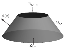
Figure 3. The Surfaces of Integration in Lemma 7.2.2

Here, $\hat{n}(x)$ is the Euclidean outer normal at $x\in M_{t,r}$ to the mantle of truncated cone, $\langle\hat{n}(x),\dot{J}(x)\rangle_{E}$ denotes the Euclidean inner product of $\hat{n}(x)$ and $\dot{J}(x)$ as vectors in $\mathbb{R}^{4},$ and $\mathcal{H}$ is the Hausdorff measure on the mantle of the cone. For each normal vector $\hat{n}(x),$ let ${}_{\hat{n}(x)}\xi$ denote the co-vector belonging to $T^{*}_{x}\mathcal{M}$ such that ${}_{\hat{n}(x)}\xi(X)={{}_{\hat{n}(x)}\xi_{\mu}}X^{\mu}=\langle\hat{n}(x),X\rangle_{E}$ holds for every $X\in T_{x}\mathcal{M}.$ By the positivity condition (5.5.2), co-vectors $\xi$ belonging to $\mathcal{I}^{*+}_{x}$ satisfy $\xi_{\mu}\dot{J}^{\mu}(\dot{\mathbf{V}},\dot{\mathbf{V}})>0$ for all non-zero variations $\dot{\mathbf{V}}.$ Since for each $x\in M_{t,r},$ the co-vector ${}_{\hat{n}(x)}\xi$ belongs to the boundary of $\mathcal{I}^{*+}_{x}$, which is the positive component of the cone $C^{*}_{x,l},$ continuity in the variable $\xi$ implies that $\langle\hat{n}(x),\dot{J}(x)\rangle_{E}\ ={{}_{\hat{n}(x)}\xi_{\mu}}\dot{J}^{\mu}(\dot{\mathbf{V}},\dot{\mathbf{V}})\geq 0$ holds for $x\in M_{t,r}.$ Furthermore, if $t_{1}<t_{2}$, then $M_{t_{1},r}\subset M_{t_{2},r}.$ From these facts it follows that $-\underset{M_{t,r}}{\int}\langle\hat{n}(x),\dot{J}(x)\rangle_{E}\,d\mathcal{H}(x)$ is a decreasing function of $t$ on $[0,T].$ Lemma 7.2.2 now follows from differentiating each side of (7.2.24) with respect to $t$ and accounting for this decreasing term. Fig. 3 illustrates the setup in $\mathbb{R}^{1+2},$ where the vertical direction represents positive values of $t.$ ∎

Returning to the proof of the proposition and recalling that we are using definitions (7.2.12) and (7.2.14) to define $\dot{\mathbf{V}}$ and $\widetilde{\mathbf{V}},$ we let $\dot{J}_{\vec{\alpha}}$ denote the energy current for the variation $\partial_{\vec{\alpha}}\dot{\mathbf{V}}$ defined by the bgs $\widetilde{\mathbf{V}}.$ For notational convenience, we allow $\vec{\alpha}$ to take on the value $\vec{\mathbf{0}},$ in which case $\dot{J}_{\vec{\mathbf{0}}}$ is defined to be the energy current in the variation $\dot{\mathbf{V}}$ defined by the bgs $\widetilde{\mathbf{V}}.$

As in Lemma 7.2.2, we define for any $T_{*}>0$ and $r>T_{*}$ the following functions of $t$ on $[0,T_{*}]:$

$$\mathscr{E}_{\vec{\alpha}}(t;r) \overset{\mbox{\tiny{def}}}{=}\Big{(}\underset{\Sigma_{t,r-t}}{\int}{\dot{J}_{\vec{\alpha}}}^{0}(t,\mathbf{s})\,d^{3}\mathbf{s}\Big{)}^{1/2}$$

(7.2.25) $$E(t;r;N) \overset{\mbox{\tiny{def}}}{=}\Big{(}\sum_{0\leq|\vec{\alpha}|\leq N}\mathscr{E}_{\vec{\alpha}}^{2}(t;r)\Big{)}^{\frac{1}{2}}=\Big{(}\sum_{0\leq|\vec{\alpha}|\leq N}\underset{\Sigma_{t,r-t}}{\int}{\dot{J}_{\vec{\alpha}}}^{0}(t,\mathbf{s})\,d^{3}\mathbf{s}\Big{)}^{\frac{1}{2}}.$$

Then with $C_{\bar{\mathcal{O}}_{2}}$ defined in (6.2.2), we have that

(7.2.26) $$C_{\bar{\mathcal{O}}_{2}}E^{2}(t;r;N) \leq\|\dot{\mathbf{V}}(t)\|_{H^{N}(\Sigma_{t,r-t})}^{2}\leq C_{\bar{\mathcal{O}}_{2}}^{-1}E^{2}(t;r;N).$$

Additionally, by Lemma 7.2.2, we have the following inequality for $0\leq t\leq T_{*}:$

(7.2.27) $$2E(t;r;N)\frac{d}{dt}E(t;r;N)\leq\sum_{0\leq|\vec{\alpha}|\leq N}{}\underset{\Sigma_{t,r-t}}{\int}\partial_{\mu}\left({\dot{J}_{\vec{\alpha}}}^{\mu}(t,\mathbf{s})\right)\,d^{3}\mathbf{s}.$$

The technically cumbersome aspect of the proof of Proposition 7.2.1 is bounding the right-hand side of (7.2.27) by a constant times $E(t;r;N)+E^{2}(t;r;N),$ which then allows us to use Gronwall’s inequality to exponentially bound from above the growth of $E(t;r;N)$ in $t.$ We prove some of the technical points in lemmas 7.3.1 and 7.3.2 below, so as to not disrupt the main argument. The keys to proofs of lemmas 7.3.1 and 7.3.2 are Sobolev-Moser calculus inequalities, special versions of which are stated in the Appendix. In the following argument, $C=C(N,\bar{\mathcal{O}}_{2},\|{{}^{(0)}\mathring{\mathbf{V}}}\|_{H_{\bar{\mathbf{V}}}^{N+1}},\Lambda,L),$ even though we have not yet chosen $L.$ By Lemma 7.3.1, we have that

$$\sum_{0\leq|\vec{\alpha}|\leq N}{}\underset{\Sigma_{t,r-t}}{\int}\partial_{\mu}\left({\dot{J}_{\vec{\alpha}}}^{\mu}(t,\mathbf{s})\right)\,d^{3}\mathbf{s} \leq C\cdot\big{[}\|\dot{\mathbf{V}}(t)\|_{H^{N}(\Sigma_{t,r-t})}+\|\dot{\mathbf{V}}(t)\|_{H^{N}(\Sigma_{t,r-t})}^{2}\big{]}$$

(7.2.28) $$\leq C\cdot\big{[}C^{-1/2}_{\bar{\mathcal{O}}_{2}}E(t;r;N)+C^{-1}_{\bar{\mathcal{O}}_{2}}E^{2}(t;r;N)\big{]},$$

where in the second inequality we have used (7.2.26). Combining (7.2.27) with (7.2.3), and applying Gronwall’s inequality, we have for $0\leq t\leq T_{*}$ that

(7.2.29) $$E(t;r;N)\leq\big{[}E(0;r;N)+C\cdot(2C_{\bar{\mathcal{O}}_{2}})^{-1/2}t\big{]}\cdot\big{[}\mbox{exp}\big{(}C\cdot(2C_{\bar{\mathcal{O}}_{2}})^{-1}t\big{)}\big{]},$$

and consequently by (7.2.26), that

(7.2.30) $$\|\dot{\mathbf{V}}(t)\|_{H^{N}(\Sigma_{t,r-t})} \leq{C_{\bar{\mathcal{O}}_{2}}^{-1}}\big{[}\|\dot{\mathbf{V}}(0)\|_{H^{N}(\Sigma_{0,r})}+Ct\big{]}\cdot\big{[}\mbox{exp}\big{(}Ct\big{)}\big{]}.$$

Letting $r\to\infty,$ taking the $\sup$ over $t\in[0,T_{*}],$ and using (7.2.9), we have that

$$\mid\mid\mid\dot{\mathbf{V}}\mid\mid\mid_{H^{N},T_{*}}\leq C^{-1}_{\bar{\mathcal{O}}_{2}}\big{[}\|\dot{\mathbf{V}}(0)\|_{H^{N}}+CT_{*}\big{]}\cdot\mbox{exp}\big{(}CT_{*}\big{)}$$

(7.2.31) $$\leq\big{[}\Lambda/2+C(N,\bar{\mathcal{O}}_{2},\|{{}^{(0)}\mathring{\mathbf{V}}}\|_{H_{\bar{\mathbf{V}}}^{N+1}},\Lambda,L)\cdot T_{*}\big{]}\cdot\mbox{exp}\big{(}C(N,\bar{\mathcal{O}}_{2},\|{{}^{(0)}\mathring{\mathbf{V}}}\|_{H_{\bar{\mathbf{V}}}^{N+1}},\Lambda,L)\cdot T_{*}\big{)}.$$

To make a viable choice of $L,$

(7.2.32) $$\mbox{we first \emph{assume} that right-hand side of \eqref{E:IterateInequality} is}\ \leq\Lambda,$$

which implies the inductive step (7.2.11a) for ${{}^{(m+1)}\mathbf{V}}$. Using assumption (7.2.32) as a hypothesis, Lemma 7.3.2 implies that there exists an $L(N,\bar{\mathcal{O}}_{2},\|{{}^{(0)}\mathring{\mathbf{V}}}\|_{H_{\bar{\mathbf{V}}}^{N}},\Lambda)>0$ such that

(7.2.33) $$\mid\mid\mid\partial_{t}\big{(}{{}^{(m+1)}\mathbf{V}}\big{)}\mid\mid\mid_{H^{N-1},T_{*}}\leq L.$$

For this fixed choice of $L,$ we can implicitly solve for a $T_{*}>0$ such that the right-hand side of inequality (7.2.3) is in fact $\leq\Lambda,$ thus justifying the assumption (7.2.32) and the conclusion (7.2.33), thereby closing the induction argument. This completes the proof of Proposition 7.2.1.

$\Box$

7.3. Proofs of Lemma 7.3.1 and Lemma 7.3.2

We now state and prove the two technical lemmas quoted in the proof of Proposition 7.2.1.

Lemma 7.3.1.

Assume the hypotheses and notation of Proposition 7.2.1. In addition, assume that
$\|\partial_{t}\widetilde{\mathbf{V}}(t)\|_{H^{N-1}}\leq L.$ Then

(7.3.1) $$\|\partial_{\mu}{\dot{J}_{\vec{\alpha}}}^{\mu}(t)\|_{L^{1}(\Sigma_{t,r-t})}\leq C(N,\bar{\mathcal{O}}_{2},\|{{}^{(0)}\mathring{\mathbf{V}}}\|_{H_{\bar{\mathbf{V}}}^{N+1}},\Lambda,L)\cdot\left(\|\dot{\mathbf{V}}(t)\|_{H^{N}}+\|\dot{\mathbf{V}}(t)\|_{H^{N}}^{2}\right).$$

Proof.

We use here the definitions (7.2.12) and (7.2.14) from Proposition 7.2.1. Recall that $\partial_{\vec{\alpha}}\dot{\mathbf{V}}$ is a solution to the EOV defined by the bgs $\widetilde{\mathbf{V}}$ with inhomogeneous terms $(\mathbf{b}_{\vec{\alpha}},\partial_{\vec{\alpha}}\mathbf{l}),$ and that $\dot{J}_{\vec{\alpha}}$ is the energy current for $\partial_{\vec{\alpha}}\dot{\mathbf{V}}$ defined by the bgs $\widetilde{\mathbf{V}}.$ Furthermore,

(7.3.2) $$\|\widetilde{\mathbf{V}}-{{}^{(0)}\mathring{\mathbf{V}}}\|_{H^{N}}\leq\Lambda$$

holds by the induction assumption from the proposition.

By (5.5.3) and Remark 5.5.3, the expression for $\partial_{\mu}{\dot{J}_{\vec{\alpha}}}^{\mu}$ consists of terms that are either precisely linear or precisely quadratic in the components of the variation $\partial_{\vec{\alpha}}\dot{\mathbf{V}}.$ The coefficients of the quadratic variation terms are smooth functions with arguments $\widetilde{\mathbf{V}}$ and $D\widetilde{\mathbf{V}}.$ Examining the particular form of these coefficients and using the fact that $\widetilde{\mathbf{V}}([0,T]\times\mathbb{R}^{3})\subset\bar{\mathcal{O}}_{2},$ we see that their $L^{\infty}$ norm is bounded by $C(\bar{\mathcal{O}}_{2})\|D\widetilde{\mathbf{V}}\|_{L^{\infty}}.$ By assumption, $\|\widetilde{\mathbf{V}}-{{}^{(0)}\mathring{\mathbf{V}}}\|_{H^{N}}\leq\Lambda$ and $\|\partial_{t}\widetilde{\mathbf{V}}(t)\|_{H^{N-1}}\leq L.$ Therefore, by Sobolev embedding, $\|D\widetilde{\mathbf{V}}\|_{L^{\infty}}\leq C(N,\|{{}^{(0)}\mathring{\mathbf{V}}}\|_{H_{\bar{\mathbf{V}}}^{N}},\Lambda,L).$ These facts imply that the $L^{1}(\Sigma_{t,r-t})$ norm of the terms involving the quadratic variations is bounded from above by $C(N,\bar{\mathcal{O}}_{2},\|{{}^{(0)}\mathring{\mathbf{V}}}\|_{H_{\bar{\mathbf{V}}}^{N}},\Lambda,L)\|\partial_{\vec{\alpha}}\dot{\mathbf{V}}\|_{L^{2}(\Sigma_{t,r-t})}^{2}.$

The coefficients of the linear variation terms are linear combinations of products of the components of $(\mathbf{b}_{\vec{\alpha}},\partial_{\vec{\alpha}}\mathbf{l}),$ where $\mathbf{b}_{\vec{\alpha}}$ is defined in (7.2.21), with smooth functions, the arguments of which are the components of $\widetilde{\mathbf{V}}.$ Since
$\widetilde{\mathbf{V}}([0,T]\times\mathbb{R}^{3})\subset\bar{\mathcal{O}}_{2},$ the smooth functions of $\widetilde{\mathbf{V}}$ are bounded in $L^{\infty}$ by $C(\bar{\mathcal{O}}_{2}).$ Therefore, by the Cauchy-Schwarz integral inequality for $L^{2},$ the $L^{1}(\Sigma_{t,r-t})$ norm of the terms depending linearly on the variations is bounded from above by $C(\bar{\mathcal{O}}_{2})\|(\mathbf{b}_{\vec{\alpha}},\partial_{\vec{\alpha}}\mathbf{l})\|_{L^{2}}\|\partial_{\vec{\alpha}}\dot{\mathbf{V}}\|_{L^{2}(\Sigma_{t,r-t})}.$ To complete the proof of (7.3.1), it remains to show that for $0\leq|{\vec{\alpha}}|\leq N,$ we have that

(7.3.3) $$\|(\mathbf{b}_{\vec{\alpha}},\partial_{\vec{\alpha}}\mathbf{l})\|_{L^{2}}\leq C(N,\bar{\mathcal{O}}_{2},\|{{}^{(0)}\mathring{\mathbf{V}}}\|_{H_{\bar{\mathbf{V}}}^{N+1}},\Lambda)\cdot\big{(}1+\|\dot{\mathbf{W}}\|_{H^{N}}\big{)}.$$

The proof of (7.3.3) will follow easily from the propositions given in the Appendix.

Concerning ourselves with the $\|\mathbf{b}_{\vec{\alpha}}\|_{L^{2}}$ estimate first, we claim that the term $A^{0}\partial_{\vec{\alpha}}\left((A^{0})^{-1}\mathbf{b}\right)$ from (7.2.21) satisfies

(7.3.4) $$\|A^{0}\partial_{\vec{\alpha}}\left((A^{0})^{-1}\mathbf{b}\right)\|_{L^{2}}\leq C(N,\bar{\mathcal{O}}_{2},\|{{}^{(0)}\mathring{\mathbf{V}}}\|_{H_{\bar{\mathbf{V}}}^{N+1}},\Lambda).$$

We repeat for clarity that $\mathbf{b}=(f,g,h^{1},h^{2},h^{3}),$ where the scalar-valued quantities $f,g,h^{1},h^{2},h^{3}$ are defined in (7.2.15) - (7.2.17). Since $\|A^{0}(\widetilde{\mathbf{V}})\|_{L^{\infty}}\leq C(\bar{\mathcal{O}}_{2}),$ to prove (7.3.4), it suffices to control the $L^{2}$ norm of $\partial_{\vec{\alpha}}\big{(}(A^{0})^{-1}\mathbf{b}\big{)}.$ Using Proposition A.2 and Remark A.1, with $(A^{0})^{-1}$ playing the role of $F$ in the proposition and $\mathbf{b}$ playing the role of $G,$ we have that

(7.3.5) $$\|\partial_{\vec{\alpha}}\big{(}(A^{0})^{-1}\mathbf{b}\big{)}\|_{L^{2}}\leq\|(A^{0})^{-1}\mathbf{b}\|_{H^{N}}\leq C(N,\bar{\mathcal{O}}_{2},\|{{}^{(0)}\mathring{\mathbf{V}}}\|_{H_{\bar{\mathbf{V}}}^{N}},\Lambda)\|\mathbf{b}\|_{H^{N}}.$$

Furthermore, Proposition A.2 and Remark A.1 imply that

(7.3.6) $$\|\mathbf{b}\|_{H^{N}}\leq C(N,\bar{\mathcal{O}}_{2},\|{{}^{(0)}\mathring{\mathbf{V}}}\|_{H_{\bar{\mathbf{V}}}^{N+1}},\Lambda).$$

Combining (7.3.5) with (7.3.6) proves (7.3.4).

We next claim that the $\mathbf{k}_{\vec{\alpha}}$ from (7.2.22) satisfy

(7.3.7) $$\|\mathbf{k}_{\vec{\alpha}}\|_{L^{2}}\leq C(N,\bar{\mathcal{O}}_{2},\|{{}^{(0)}\mathring{\mathbf{V}}}\|_{H_{\bar{\mathbf{V}}}^{N}},\Lambda)\|\dot{\mathbf{W}}\|_{H^{N}}.$$

Again, since $\|A^{0}(\widetilde{\mathbf{V}})\|_{L^{\infty}}\leq C(\bar{\mathcal{O}}_{2}),$ to prove (7.3.7), it suffices to control the $L^{2}$ norm of $(A^{0})^{-1}A^{k}\partial_{k}(\partial_{\vec{\alpha}}\dot{\mathbf{W}})-\partial_{\vec{\alpha}}\left((A^{0})^{-1}A^{k}\partial_{k}\dot{\mathbf{W}}\right).$ By Proposition A.5 and Remark A.3, with $(A^{0})^{-1}A^{k}$ playing the role of $F$ in the proposition, and $\partial_{k}\dot{\mathbf{W}}$ playing the role of $G,$ we have that

(7.3.8) $$\|(A^{0})^{-1}A^{k}\partial_{k}(\partial_{\vec{\alpha}}\dot{\mathbf{W}})-\partial_{\vec{\alpha}}\big{(}(A^{0})^{-1}A^{k}\partial_{k}\dot{\mathbf{W}}\big{)}\|_{L^{2}}$$

$$\leq C(N,\bar{\mathcal{O}}_{2},\|{{}^{(0)}\mathring{\mathbf{V}}}\|_{H_{\bar{\mathbf{V}}}^{N}},\Lambda)\|\nabla^{(1)}\dot{\mathbf{W}}\|_{H^{N-1}},$$

from which (7.3.7) immediately follows.

To finish the proof of (7.3.3), we will show that

(7.3.9) $$\|l^{(z)}\|_{H^{N}}\leq C(N,\bar{\mathcal{O}}_{2},\|{{}^{(0)}\mathring{\mathbf{V}}}\|_{H_{\bar{\mathbf{V}}}^{N+1}},\Lambda)\qquad(z=0,1,2,3,4).$$

For $l^{(1)},l^{(2)},l^{(3)},l^{(4)}$ defined in (7.2.19) and (7.2.20), the claim is trivial. To estimate the component $l^{(0)},$ defined in (7.2.18), we first rewrite

(7.3.10) $$l^{(0)}=\kappa^{2}(\widetilde{\phi}-\bar{\phi})+(\widetilde{R}-\bar{R})-3(\widetilde{P}-\bar{P})-\partial^{k}[{{}^{(0)}\mathring{\psi}_{k}}],$$

where $\bar{P}\overset{\mbox{\tiny{def}}}{=}e^{4\bar{\phi}}\bar{p}$ and $\bar{R}\overset{\mbox{\tiny{def}}}{=}e^{4\bar{\phi}}\mathscr{R}(e^{-4\bar{\phi}}\bar{P},\bar{{{\eta}}}),$ the function $\mathscr{R}$ is defined in (4.1.5), and $\bar{p}$ and $\bar{{{\eta}}}$ are constants defined in Section 6. In equation (7.3.10), we have made use of (6.1.2), which is the assumption that $\kappa^{2}\bar{\phi}+\bar{R}-3\bar{P}=0.$ Since

(7.3.11) $$\|\kappa^{2}(\widetilde{\phi}-\bar{\phi})\|_{H^{N}}+3\|(\widetilde{P}-\bar{P})\|_{H^{N}}+\|\partial^{k}[{{}^{(0)}\mathring{\psi}_{k}}]\|_{H^{N}}\leq C(\|{{}^{(0)}\mathring{\mathbf{V}}}\|_{H_{\bar{\mathbf{V}}}^{N+1}},\Lambda),$$

we only need to show that

(7.3.12) $$\|\widetilde{R}-\bar{R}\|_{H^{N}}\leq C(N,\bar{\mathcal{O}}_{2},\|{{}^{(0)}\mathring{\mathbf{V}}}\|_{H_{\bar{\mathbf{V}}}^{N}},\Lambda).$$

This follows immediately from definition (4.2.10), Proposition A.4, and Remark A.2.

Inequality (7.3.3) now follows from combining (7.2.21), (7.3.4), (7.3.7), and (7.3.9); this completes the proof of (7.3.1). ∎

Lemma 7.3.2.

Assume the hypotheses and notation of Proposition 7.2.1. Also assume the induction hypothesis $\mid\mid\mid{{}^{(m)}\mathbf{V}}-{{}^{(0)}\mathring{\mathbf{V}}}\mid\mid\mid_{H^{N},T_{*}}\leq\Lambda$ from Proposition 7.2.1. Assume further that $\mid\mid\mid{{}^{(m+1)}\mathbf{V}}-{{}^{(0)}\mathring{\mathbf{V}}}\mid\mid\mid_{H^{N},T_{*}}\leq\Lambda.$ Then

(7.3.13) $$\mid\mid\mid\partial_{t}\big{(}{{}^{(m+1)}\mathbf{V}}\big{)}\mid\mid\mid_{H^{N-1},T_{*}}\leq L(N,\bar{\mathcal{O}}_{2},\|{{}^{(0)}\mathring{\mathbf{V}}}\|_{H_{\bar{\mathbf{V}}}^{N}},\Lambda).$$

Proof.

By Remark 4.2.2, we may solve for $\partial_{t}({{}^{(m+1)}\mathbf{W}}):$

(7.3.14) $$\partial_{t}\big{(}{{}^{(m+1)}\mathbf{W}}\big{)}=\big{(}A^{0}({{}^{(m)}\mathbf{V}})\big{)}^{-1}\big{(}\mathbf{b}-A^{k}({{}^{(m)}\mathbf{V}})\partial_{k}({{}^{(m+1)}\mathbf{W}})\big{)},$$

where the function $\mathbf{b}$ denotes the inhomogeneous terms from the linearized EN_κ equations satisfied by ${{}^{(m+1)}\mathbf{W}};$ i.e., $\mathbf{b}{=}\boldsymbol{\mathfrak{B}}({{}^{(m)}\mathbf{V}}),$ where

(7.3.15) $$\boldsymbol{\mathfrak{B}}(\cdot)\overset{\mbox{\tiny{def}}}{=}\left(\mathfrak{F}(\cdot),\mathfrak{G}(\cdot),\mathfrak{H}^{(1)}(\cdot),\mathfrak{H}^{(2)}(\cdot),\mathfrak{H}^{(3)}(\cdot)\right)$$

is an array-valued function, the scalar-valued functions $\mathfrak{F},\mathfrak{G},\cdots,\mathfrak{H}^{(3)}$ are defined in (4.2.11) - (4.2.13), and the $A^{\mu}(\cdot)$ are defined in (4.2.19).

Using the hypotheses of the lemma, we apply Proposition A.2 and Remark A.1 to the right-hand side of (7.3.14), concluding that

(7.3.16) $$\mid\mid\mid\partial_{t}\big{(}{{}^{(m+1)}\mathbf{W}}\big{)}\mid\mid\mid_{H^{N-1},T_{*}}\leq L(N,\bar{\mathcal{O}}_{2},\|{{}^{(0)}\mathring{\mathbf{V}}}\|_{H_{\bar{\mathbf{V}}}^{N}},\Lambda).$$

Likewise, an argument similar to the one used to prove (7.3.9) gives that

(7.3.17) $$\mid\mid\mid\partial_{t}\big{(}{{}^{(m+1)}\phi},{{}^{(m+1)}\psi_{0}},\cdots,{{}^{(m+1)}\psi_{3}}\big{)}\mid\mid\mid_{H^{N-1},T_{*}}\leq L(N,\bar{\mathcal{O}}_{2},\|{{}^{(0)}\mathring{\mathbf{V}}}\|_{H_{\bar{\mathbf{V}}}^{N}},\Lambda).$$

Combining (7.3.16) and (7.3.17) proves (7.3.13). ∎

7.3.1. Uniqueness and $H^{N-1}-$Lipschitz-continuous dependence on initial data.

We now prove the prove the uniqueness of $H_{\bar{\mathbf{V}}}^{N}$ solutions to the EN_κ system and show that the solution is an $H^{N-1}-$Lipschitz-continuous function of the initial data. Let $\mathring{\mathbf{V}}$ denote initial data that launch a solution $\mathbf{V}$ of the EN_κ system as furnished by the existence aspect of Theorem 1. Let $\delta,B_{\delta}(\mathring{\mathbf{V}}),T^{\prime},$ and $K(N,\bar{\mathcal{O}}_{2},\|{{}^{(0)}\mathring{\mathbf{V}}}\|_{H_{\bar{\mathbf{V}}}^{N+1}},\Lambda,\delta)$ be as in corollaries 7.0.1 and 7.0.2. Assume that the initial data $\mathring{\widetilde{\mathbf{V}}}$ belong to $B_{\delta},$ and let $\widetilde{\mathbf{V}}$ be a solution of the EN_κ system with initial data $\mathring{\widetilde{\mathbf{V}}}$ existing on the interval $[0,T^{\prime}]$ as furnished by Corollary 7.0.1. We now define

(7.3.18) $$\dot{\mathbf{V}}\overset{\mbox{\tiny{def}}}{=}\widetilde{\mathbf{V}}-\mathbf{V}.$$

It follows from definition (7.3.18) that $\dot{\mathbf{V}}$ is a solution to the EOV (4.2.1) - (4.2.10) defined by the bgs $\widetilde{\mathbf{V}}$ with inhomogeneous terms given by (for $j=1,2,3$)

(7.3.19) $$f =(U^{\mu}-\widetilde{U}^{\mu})\partial_{\mu}{{\eta}}$$

(7.3.20) $$g =(U^{\mu}-\widetilde{U}^{\mu})\partial_{\mu}P+\big{[}QU_{k}/U^{0}-\widetilde{Q}\widetilde{U}_{k}/\widetilde{U}^{0}\big{]}\partial_{0}U^{k}$$

$$\ \ +(Q-\widetilde{Q})\partial_{k}U^{k}+(4\widetilde{P}-3\widetilde{Q})\widetilde{U}^{\mu}\widetilde{\psi}_{\mu}-(4P-3Q)U^{\mu}\psi_{\mu}$$

(7.3.21) $$h^{(j)} =\big{[}(R+P)U^{\mu}-(\widetilde{R}+\widetilde{P})\widetilde{U}^{\mu}\big{]}\partial_{\mu}U^{j}+(\Pi^{\mu j}-\widetilde{\Pi}^{\mu j})\partial_{\mu}P$$

(7.3.22) $$\ \ +(3\widetilde{P}-\widetilde{R})\widetilde{\Pi}^{\mu j}\widetilde{\psi}_{\mu}-(3P-R)\Pi^{\mu j}\psi_{\mu}$$

(7.3.23) $$l^{(0)} ={\kappa}^{2}(\widetilde{\phi}-\phi)+(\widetilde{R}-3\widetilde{P})-(R-3P)$$

(7.3.24) $$l^{(j)} =0$$

(7.3.25) $$l^{(4)} =\widetilde{\psi}_{0}-\psi_{0},$$

and we denote them using the abbreviated notation $\mathbf{b}$ and $\mathbf{l}$ defined in (4.2.17) and (4.2.18).

By combining Proposition A.2, Remark A.1, Proposition A.4, and Remark A.2 (noting the particular manner in which the inhomogeneous terms depend on the difference of functions of $\mathbf{V}$ and $\widetilde{\mathbf{V}}$), we have that

(7.3.26) $$\mid\mid\mid(\mathbf{b},\mathbf{l})\mid\mid\mid_{H^{N-1},T^{\prime}}\leq C(N,\bar{\mathcal{O}}_{2},K)\mid\mid\mid\dot{\mathbf{V}}\mid\mid\mid_{H_{\bar{\mathbf{V}}}^{N-1},T^{\prime}}.$$

Without providing details, we reason as in our proof of Proposition 7.2.1, using (7.3.26) in place of (7.3.6) and (7.3.9) to arrive at the following bound:

(7.3.27) $$\mid\mid\mid\dot{\mathbf{V}}\mid\mid\mid_{H_{\bar{\mathbf{V}}}^{N-1},T^{\prime}} \leq C^{-1}_{\bar{\mathcal{O}}_{2}}\|\dot{\mathbf{V}}(0)\|_{H^{N-1}}\cdot\mbox{exp}\big{(}C(N,\bar{\mathcal{O}}_{2},K)\cdot T^{\prime}\big{)},$$

where $\dot{\mathbf{V}}(0)\overset{\mbox{\tiny{def}}}{=}\mathring{\widetilde{\mathbf{V}}}-\mathring{\mathbf{V}}.$

We now observe that (7.3.27) implies both the uniqueness statement in Theorem 1 and the $H^{N-1}-$Lipschitz-continuous dependence on the initial data mentioned in Remark 7.0.2.

Remark 7.3.1.

We cannot obtain an estimate analogous to (7.3.27) by using the $H_{\bar{\mathbf{V}}}^{N}$ norm in place of the $H_{\bar{\mathbf{V}}}^{N-1}$ norm; the inhomogeneous terms (7.3.19) - (7.3.25) already contain one derivative of $\mathbf{V},$ and therefore cannot be bounded in the $H_{\bar{\mathbf{V}}}^{N}$ norm. However, for $N^{\prime}<N,$ we can obtain an estimate for the $H_{\bar{\mathbf{V}}}^{N^{\prime}}$ norm by combining Proposition A.6, (7.3.27) and the uniform bound provide by the constant $K.$ The inequality we obtain is

(7.3.28) $$\mid\mid\mid\dot{\mathbf{V}}\mid\mid\mid_{H_{\bar{\mathbf{V}}}^{N^{\prime}},T^{\prime}} \leq C\|\dot{\mathbf{V}}(0)\|^{1-N^{\prime}/N}_{H^{N^{\prime}}}\cdot\mbox{exp}\left(CT^{\prime}\right),$$

where in (7.3.28), $C=C(N^{\prime},N,\bar{\mathcal{O}}_{2},K).$

Remark 7.3.2.

The estimate (7.3.27) is a limiting version of the “conical” estimate

(7.3.29) $$\|\dot{\mathbf{V}}(t)\|_{H^{N-1}(\Sigma_{t,r-t})} \leq C^{-1}_{\bar{\mathcal{O}}_{2}}\|\dot{\mathbf{V}}(0)\|_{H^{N-1}(\Sigma_{0,r})}\cdot\mbox{exp}\left(Ct\right),$$

where we are using notation defined in Lemma 7.2.2. A proof of (7.3.29) can be constructed using arguments similar to the ones used in our proof of (7.2.30). Inequality (7.3.29) shows that two solutions that agree on $\Sigma_{0,r}$ also agree on $\Sigma_{t,r-t}.$ By translating the cone from Lemma 7.2.2 so that its lower base is centered at the spacetime point $x,$ we may produce a translated version of the inequality. Thus, we observe that a domain of dependence for $x\in\mathcal{M}$ is given by the solid backward light cone in $\mathcal{M}$ with vertex at $x;$ i.e., the past (relative to $x$) behavior of a solution to the EOV outside of this cone does not influence behavior of the solution at $x.$ Similarly, a domain of influence of $x$ is the solid forward light cone with vertex at $x;$ the behavior of a solution at $x$ does not influence the future (relative to $x$) behavior of the solution outside of this cone, a fact which justifies our claim made in Section 5.4 that the fastest speed of propagation in the EN_κ system is the speed of light. In [6], Christodoulou gives an advanced discussion of these and related topics for hyperbolic PDEs derivable from a Lagrangian.

This completes our abbreviated proof of Theorem $\ref{T:LocalExistence}.$

$\Box$

7.4. Proof of Theorem 2.

We now provide a detailed proof of Theorem 2.

7.4.1. The setup

Let $\{\mathring{\mathbf{V}}^{m}\}$ be the sequence of initial data from the hypotheses of Theorem 2 converging in $H_{\bar{\mathbf{V}}}^{N}$ to $\mathring{\mathbf{V}}$ . By corollaries 7.0.1 and 7.0.2, for all large $m,$ the initial data $\mathring{\mathbf{V}}^{m}$ and $\mathring{\mathbf{V}}$ launch unique solutions $\mathbf{V}^{m}$ and $\mathbf{V}$ respectively to (4.1.18) - (4.1.26) that exist on a common interval $[0,T^{\prime}]$ and that have the property
$\mathbf{V}([0,T^{\prime}]\times\mathbb{R}^{3})\subset\bar{\mathcal{O}}_{2},\mathbf{V}^{m}([0,T^{\prime}]\times\mathbb{R}^{3})\subset\bar{\mathcal{O}}_{2}.$ Furthermore, for all large $m,$ with
$K=K(N,\bar{\mathcal{O}}_{2},\|{{}^{(0)}\mathring{\mathbf{V}}}\|_{H_{\bar{\mathbf{V}}}^{N+1}},\Lambda,\delta),$ we have the uniform (in $m$) bounds

(7.4.1) $$\mid\mid\mid\mathbf{V}\mid\mid\mid_{H_{\bar{\mathbf{V}}}^{N},T},\mid\mid\mid\partial_{t}\mathbf{V}\mid\mid\mid_{H^{N-1},T},\mid\mid\mid\mathbf{V}^{m}\mid\mid\mid_{H_{\bar{\mathbf{V}}}^{N},T^{\prime}},\mid\mid\mid\partial_{t}\mathbf{V}^{m}\mid\mid\mid_{H^{N-1},T^{\prime}}\ <\ K,$$

where $[0,T]$ is the interval of existence for $\mathbf{V}$ furnished by Theorem 1. In this section, we will show that for all large $m,\mathbf{V}^{m}$ exists on $[0,T]$ and that

(7.4.2) $$\lim_{m\to\infty}\mid\mid\mid\mathbf{V}^{m}-\mathbf{V}\mid\mid\mid_{H^{N},T}=0.$$

The proof we give here is inspired by a similar proof given by Kato in [18]. We use results and terminology from the theory of abstract evolution equations in Banach spaces, an approach that streamlines the argument. We also freely use results from the theory of integration in Banach spaces; a detailed discussion of this theory may be found in [34]. We begin by rewriting the linearization of the EN_κ system around $\mathbf{V}$ and $\mathbf{V}^{m}$ as abstract evolution equations in the affine Banach space $H_{\bar{\mathbf{V}}}^{N}(\mathbb{R}^{3}).$ In this form, the linearized systems are respectively written as

(7.4.3) $$\partial_{t}\mathbf{Z}+\mathcal{A}(\mathbf{V})\mathbf{Z}=\mathbf{f}(\mathbf{V})$$

(7.4.4) $$\partial_{t}\mathbf{Z}+\mathcal{A}(\mathbf{V}^{m})\mathbf{Z}=\mathbf{f}(\mathbf{V}^{m}),$$

where $\mathbf{f}(\cdot)$ is a smooth function on $\mathcal{O},$ and $\mathbf{f}(\bar{\mathbf{V}})=\mathbf{0}.$ Here, the symbol $\mathbf{Z}$ stands for all 10 components of a solution to a linearized system, and the operator $\mathcal{A}(\cdot)$ is a first order spatial differential operator with coefficients that depend smoothly on its arguments. We state for clarity that the first 5 components of the inhomogeneous terms $\mathbf{f}(\mathbf{V}^{m})$ are given by $\left(A^{0}(\mathbf{V}^{m})\right)^{-1}\cdot(\mathfrak{F}(\mathbf{V}^{m}),\mathfrak{G}(\mathbf{V}^{m}),\cdots,\mathfrak{H}^{(3)}(\mathbf{V}^{m}))^{Transpose},$ where the matrix-valued function $A^{0}(\cdot)$ is defined in (4.2.20) and the scalar-valued functions $\mathfrak{F},\mathfrak{G},\cdots\mathfrak{H}^{3}$ are defined in (4.2.11) - (4.2.13).

We will make use of the pseudodifferential operator

(7.4.5) $$\mbox{{S}}\overset{\mbox{\tiny{def}}}{=}(1-\Delta)^{N/2},$$

which is an isomorphism between $H^{N}$ and $L^{2};$ i.e., $\mbox{{S}}\in\mathcal{L}(H^{N},L^{2})$ and
$\mbox{{S}}^{-1}\in\mathcal{L}(L^{2},H^{N}).$

7.4.2. Technical estimates

In this section, we provide some technical lemmas that will be needed in our proof of Theorem 2. For certain function spaces $X,$ there exist evolution operators

(7.4.6) $$\mathcal{U}(t,t^{\prime}),\ \mathcal{U}^{m}(t,t^{\prime}):X\rightarrow X$$

defined on $\triangle_{T^{\prime}}\overset{\mbox{\tiny{def}}}{=}\{0\leq t^{\prime}\leq t\leq T^{\prime}\}$ that map solutions (belonging to the space $X$) of the corresponding homogeneous version of the linearized systems (7.4.3) and (7.4.4) at time $t^{\prime}$ to solutions at time $t.$ The relevant spaces in our discussion are $X=L^{2}$ and $X=H^{N}.$ In the following three lemmas, we describe the properties of the operators $\mathcal{U}(t,t^{\prime})$ and $\mathcal{U}^{m}(t,t^{\prime}).$ Complete proofs are given in [16], [17], and [18]; rather than repeating them, we instead attempt to provide some insight into how the proofs relate to the methods described in this paper.

Lemma 7.4.1.

$\mathcal{U}(\cdot,\cdot)$ and $\mathcal{U}^{m}(\cdot,\cdot)$ (for $m\geq 0$) are strongly-continuous maps from $\triangle_{T^{\prime}}$ into $\mathcal{L}(L^{2})\cap\mathcal{L}(H^{N}).$ Furthermore, there exists a $C(K)>0$ such that $\mid\mid\mid\mathcal{U}\mid\mid\mid_{L^{2},\triangle_{T^{\prime}}},\mid\mid\mid\mathcal{U}^{m}\mid\mid\mid_{L^{2},\triangle_{T^{\prime}}},\mid\mid\mid\mathcal{U}\mid\mid\mid_{H^{N},\triangle_{T^{\prime}}},\mid\mid\mid\mathcal{U}^{m}\mid\mid\mid_{H^{N},\triangle_{T^{\prime}}}<C(K).$

Remark 7.4.1.

Lemma 7.4.1 is essentially a consequence of the fact that the uniform bound (7.4.1) for $\mathbf{V}$ and $\mathbf{V}^{m}$ allows for uniform Sobolev estimates to be made on the $L^{2}$ (or $H^{N}$) norm of $L^{2}$ (or $H^{N}$) solutions to the linearized equations.

Remark 7.4.2.

By the regularity result of $\mathbf{V}$ furnished by Theorem 1, Corollary A.3, Remark A.1, and (6.1.2), the right-hand side (7.4.3) is an element of $C^{0}([0,T],H^{N}).$ Given a function $\mathring{\mathbf{Z}}\in H_{\bar{\mathbf{V}}}^{N},$ it follows from Lemma 7.4.1 and standard linear theory (via Duhamel’s principle) that there exists a unique solution $\mathbf{Z}\in C^{0}([0,T],H_{\bar{\mathbf{V}}}^{N})$ to (7.4.3) with initial data equal to $\mathring{\mathbf{Z}}.$ An analogous result holds for solutions to (7.4.4).

Lemma 7.4.2.

$\mathcal{U}^{m}(t,t^{\prime})$ converges to $\mathcal{U}(t,t^{\prime})$ strongly in $\mathcal{L}(L^{2})$ as $m\to\infty.$ Furthermore, the strong convergence is uniform on $\triangle_{T^{\prime}}.$

Remark 7.4.3.

By smoothing the initial data, a solution $\mathbf{Z}\in C^{0}([0,T],L^{2})$ to either $\partial_{t}\mathbf{Z}+\mathcal{A}(\mathbf{V})\mathbf{Z}=0$ or $\partial_{t}\mathbf{Z}+\mathcal{A}(\mathbf{V}^{m})\mathbf{Z}=\mathbf{f}(\mathbf{V}^{m})$ can be realized as the limit (in the norm $\mid\mid\mid\cdot\mid\mid\mid_{L^{2},T}$) of a sequence $\{\mathbf{Z}^{k}\}\subset C^{0}([0,T],H^{N}).$ Therefore, to prove Lemma 7.4.2, one only needs to check that given initial data $\mathring{\mathbf{Z}}\in H^{N},$ we have that

(7.4.7) $$\lim_{m\to\infty}\mid\mid\mid\big{(}\mathcal{U}^{m}(\cdot,0)-\mathcal{U}(\cdot,0)\big{)}\mathring{\mathbf{Z}}\mid\mid\mid_{L^{2},T}=0.$$

Based on Lemma 7.4.1 and (7.3.28), which can be used to show that for $N^{\prime}<N$ we have $\mathbf{V}^{m}\rightarrow\mathbf{V}$ in $C^{0}([0,T^{\prime}],H_{\bar{\mathbf{V}}}^{N^{\prime}})\cap C_{b}^{1}([0,T^{\prime}]\times\mathbb{R}^{3}),$ (7.4.7) follows from the method of energy currents.

Lemma 7.4.3.

There exist operator-valued functions $\mathcal{B}:[0,T]\rightarrow\mathcal{L}(L^{2}),\\ \mathcal{B}^{m}:[0,T^{\prime}]\rightarrow\mathcal{L}(L^{2})$ such that

(7.4.8) $$\mbox{{S}}\mathcal{A}(\mathbf{V}(t))\mbox{{S}}^{-1}=\mathcal{A}(\mathbf{V}(t))+\mathcal{B}(t)$$

(7.4.9) $$\mbox{{S}}\mathcal{A}(\mathbf{V}^{m}(t))\mbox{{S}}^{-1}=\mathcal{A}(\mathbf{V}^{m}(t))+\mathcal{B}^{m}(t).$$

Furthermore, for all $t^{\prime}$ with $0\leq t^{\prime}\leq T^{\prime},$ $\mathcal{B}$ and $\mathcal{B}^{m}$ satisfy the estimates

(7.4.10) $$\mid\mid\mid\mathcal{B}^{m}-\mathcal{B}\mid\mid\mid_{L^{2},t^{\prime}} \leq C(K)\mid\mid\mid\mathbf{V}^{m}-\mathbf{V}\mid\mid\mid_{H^{N},t^{\prime}}$$

(7.4.11) $$\mbox{and}\ \mid\mid\mid\mathcal{B}\mid\mid\mid_{L^{2},T},\ \mid\mid\mid\mathcal{B}^{m}\mid\mid\mid_{L^{2},T^{\prime}} \leq C(K).$$

Remark 7.4.4.

A modern treatment of commutator estimates that can be used to prove Lemma 7.4.3 is located in [33].

Our proof of Theorem 2 also requires the following lemma, whose simple proof is based on Duhamel’s principle:

Lemma 7.4.4.

Let $\mathring{\mathbf{Z}}\in H_{\bar{\mathbf{V}}}^{N},$ and let $\mathbf{Z}\in C^{0}([0,T],H_{\bar{\mathbf{V}}}^{N})$ denote the unique solution to (7.4.3) with initial data equal to $\mathring{\mathbf{Z}}$ as furnished by Remark 7.4.2. Then for
$t\in[0,T],$ $\mbox{{S}}(\mathbf{Z}-\bar{\mathbf{V}})$ satisfies the Duhamel formula

$$\mbox{{S}}(\mathbf{Z}(t)-\bar{\mathbf{V}})=\mathcal{U}(t,0)\mbox{{S}}(\mathring{\mathbf{Z}}-\bar{\mathbf{V}}) -\int_{0}^{t}\mathcal{U}(t,t^{\prime})\mathcal{B}(t^{\prime})\mbox{{S}}(\mathbf{Z}(t^{\prime})-\bar{\mathbf{V}})\,dt^{\prime}$$

(7.4.12) $$+\int_{0}^{t}\mathcal{U}(t,t^{\prime})\mbox{{S}}\mathbf{f}(\mathbf{V}(t^{\prime}))\,dt^{\prime}.$$

An analogous result holds for the linearization of the EN_κ system around $\mathbf{V}^{m}.$

Proof.

We apply S to each side of the equation satisfied by $\mathbf{Z}-\bar{\mathbf{V}}$ and use Lemma 7.4.3 to arrive at the equation

(7.4.13) $$\partial_{t}\big{[}\mbox{{S}}(\mathbf{Z}-\bar{\mathbf{V}})\big{]}+\mathcal{A}(\mathbf{V})\mbox{{S}}(\mathbf{Z}-\bar{\mathbf{V}})=-\mathcal{B}(\mathbf{V})\mbox{{S}}(\mathbf{Z}-\bar{\mathbf{V}})+\mbox{{S}}\mathbf{f}(\mathbf{V}).$$

Thus, $\mbox{{S}}(\mathbf{Z}-\bar{\mathbf{V}})$ is a solution to the same linear equation that $\mathbf{Z}$ solves, except the inhomogeneous terms for $\mbox{{S}}(\mathbf{Z}-\bar{\mathbf{V}})$ are given by the right-hand side of (7.4.13) and the initial data are given by $\mbox{{S}}(\mathring{\mathbf{Z}}-\bar{\mathbf{V}}).$ Equation (7.4.4) now follows from Duhamel’s principle. Note that $\mbox{{S}}\mathbf{f}(\mathbf{V})$ is well-defined since $\mathbf{f}(\bar{\mathbf{V}})=\mathbf{0},$ and we can therefore apply Proposition A.4 and Remark A.2 to conclude that $\mathbf{f}(\mathbf{V})\in H^{N}.$ ∎

7.4.3. Proof of Theorem 2

We will now demonstrate (7.4.2) by providing a proof of the equivalent statement

(7.4.14) $$\lim_{m\to\infty}\mid\mid\mid\mbox{{S}}\left(\mathbf{V}^{m}-\mathbf{V}\right)\mid\mid\mid_{L^{2},T}=0.$$

Lemma 7.4.4 implies the following equality, valid for $0\leq t\leq T^{\prime}:$

$$\mbox{{S}}\big{(}\mathbf{V}^{m}(t)-\mathbf{V}(t)\big{)}=\mathcal{U}^{m}(t,0)\mbox{{S}}\big{(}\mathring{\mathbf{V}}^{m}-\mathring{\mathbf{V}}\big{)}+\big{(}\mathcal{U}^{m}(t,0)-\mathcal{U}(t,0)\big{)}\mbox{{S}}(\mathring{\mathbf{V}}-\bar{\mathbf{V}})$$

$$+\int_{0}^{t}\mathcal{U}(t,t^{\prime})\mathcal{B}(t^{\prime})\mbox{{S}}(\mathbf{V}(t^{\prime})-\bar{\mathbf{V}})\,dt^{\prime}-\int_{0}^{t}\mathcal{U}^{m}(t,t^{\prime})\mathcal{B}^{m}(t^{\prime})\mbox{{S}}(\mathbf{V}^{m}(t^{\prime})-\bar{\mathbf{V}})\,dt^{\prime}$$

(7.4.15) $$+\int_{0}^{t}\mathcal{U}^{m}(t,t^{\prime})\mbox{{S}}\mathbf{f}(\mathbf{V}^{m}(t^{\prime}))\,dt^{\prime}-\int_{0}^{t}\mathcal{U}(t,t^{\prime})\mbox{{S}}\mathbf{f}(\mathbf{V}(t^{\prime}))\,dt^{\prime}.$$

By Lemma 7.4.1, we have that

(7.4.16) $$\mid\mid\mid\mathcal{U}^{m}(t,0)\mbox{{S}}\big{(}\mathring{\mathbf{V}}^{m}-\mathring{\mathbf{V}}\big{)}\mid\mid\mid_{L^{2},T^{\prime}}\leq C(\mbox{{S}},K)\mid\mid\mathring{\mathbf{V}}^{m}-\mathring{\mathbf{V}}\mid\mid_{H^{N}}.$$

Furthermore, if we define

(7.4.17) $$\sup_{t\in[0,T^{\prime}]}\|\big{(}\mathcal{U}^{m}(t,0)-\mathcal{U}(t,0)\big{)}\mbox{{S}}(\mathring{\mathbf{V}}-\bar{\mathbf{V}})\|_{L^{2}}\overset{\mbox{\tiny{def}}}{=}d_{m},$$

then Lemma 7.4.2 implies that

(7.4.18) $$\lim_{m\to\infty}d_{m}=0.$$

We now rewrite the second line of (7.4.3) as

$$\int_{0}^{t}(\mathcal{U}(t,t^{\prime})-\mathcal{U}^{m}(t,t^{\prime}))\mathcal{B}(t^{\prime})\mbox{{S}}(\mathbf{V}(t^{\prime})-\bar{\mathbf{V}})\,dt^{\prime}$$

$$+ \int_{0}^{t}\mathcal{U}^{m}(t,t^{\prime})\left(\mathcal{B}(t^{\prime})-\mathcal{B}^{m}(t^{\prime})\right)\mbox{{S}}(\mathbf{V}(t^{\prime})-\bar{\mathbf{V}})\,dt^{\prime}$$

(7.4.19) $$+ \int_{0}^{t}\mathcal{U}^{m}(t,t^{\prime})\mathcal{B}^{m}(t^{\prime})\mbox{{S}}\left(\mathbf{V}(t^{\prime})-\mathbf{V}^{m}(t^{\prime})\right)\,dt^{\prime}.$$

By (7.4.1), Lemma 7.4.1 and Lemma 7.4.3, for $0\leq t\leq T_{*}\leq T^{\prime},$ the $L^{2}$ norms of the second and third integrals in (7.4.3) are each bounded from above by
$C(\mbox{{S}},K)T_{*}\mid\mid\mid\mathbf{V}^{m}-\mathbf{V}\mid\mid\mid_{H^{N},T*}.$

We similarly split the third line of (7.4.3) into two terms and use (7.4.1), Lemma 7.4.1, Proposition A.4, and Remark A.2 to bound the $L^{2}$ norm of one of them, namely $\int_{0}^{t}\mathcal{U}^{m}(t,t^{\prime})\mbox{{S}}\big{(}\mathbf{f}(\mathbf{V}^{m}(t^{\prime})-\mathbf{f}(\mathbf{V}(t^{\prime}))\big{)}\,dt^{\prime},$ from above by
$C(\mbox{{S}},K)T_{*}\mid\mid\mid\mathbf{V}^{m}-\mathbf{V}\mid\mid\mid_{H^{N},T*}.$

Combining these estimates with (7.4.16) and (7.4.17), we take the $L^{2}$ norm of each side of (7.4.3) followed by the $\sup$ over $t\in[0,T_{*}]$ to arrive at the inequality

$$\mid\mid\mid\mbox{{S}}\left(\mathbf{V}^{m}-\mathbf{V}\right)\mid\mid\mid_{L^{2},T_{*}} \leq C(\mbox{{S}},K)\|\mathring{\mathbf{V}}^{m}-\mathring{\mathbf{V}}\|_{H^{N}}+d_{m}$$

$$+C(\mbox{{S}},K)T_{*}\mid\mid\mid\mathbf{V}^{m}-\mathbf{V}\mid\mid\mid_{H^{N},T_{*}}$$

$$+\int_{0}^{T_{*}}\sup_{t\in[0,T_{*}]}\|(\mathcal{U}(t,t^{\prime})-\mathcal{U}^{m}(t,t^{\prime}))\mathcal{B}(t^{\prime})\mbox{{S}}(\mathbf{V}(t^{\prime})-\bar{\mathbf{V}})\|_{L^{2}}\,dt^{\prime}$$

(7.4.20) $$+\int_{0}^{T_{*}}\sup_{t\in[0,T_{*}]}\|(\mathcal{U}^{m}(t,t^{\prime})-\mathcal{U}(t,t^{\prime}))\mbox{{S}}\mathbf{f}(\mathbf{V}(t^{\prime}))\|_{L^{2}}\,dt^{\prime}.$$

We now choose $T_{*}$ small enough so that

(7.4.21) $$C(\mbox{{S}},K)T_{*}\mid\mid\mid\mathbf{V}^{m}-\mathbf{V}\mid\mid\mid_{H^{N},T_{*}}\leq\frac{1}{2}\mid\mid\mid\mbox{{S}}\left(\mathbf{V}^{m}-\mathbf{V}\right)\mid\mid\mid_{L^{2},T_{*}},$$

from which it follows that

$$\mid\mid\mid\mbox{{S}}\left(\mathbf{V}^{m}-\mathbf{V}\right) \mid\mid\mid_{L^{2},T_{*}}\ \leq 2C(\mbox{{S}},K)\|\mathring{\mathbf{V}}^{m}-\mathring{\mathbf{V}}\|_{H^{N}}+2d_{m}$$

$$+2\int_{0}^{T_{*}}\sup_{t\in[0,T_{*}]}\|\left(\mathcal{U}^{m}(t,t^{\prime})-\mathcal{U}(t,t^{\prime})\right)\mathcal{B}(t^{\prime})\mbox{{S}}(\mathbf{V}(t^{\prime})-\bar{\mathbf{V}})\|_{L^{2}}\,dt^{\prime}$$

(7.4.22) $$+2\int_{0}^{T_{*}}\sup_{t\in[0,T_{*}]}\|\left(\mathcal{U}^{m}(t,t^{\prime})-\mathcal{U}(t,t^{\prime})\right)\mbox{{S}}\big{(}\mathbf{f}({\mathbf{V}}(t^{\prime}))-\mathbf{f}(\bar{\mathbf{V}})\big{)}\|_{L^{2}}\,dt^{\prime},$$

where in (7.4.22), we have used the fact that $\mathbf{f}(\bar{\mathbf{V}})=\mathbf{0}.$

By (7.4.1), Lemma 7.4.1, Lemma 7.4.3, Proposition A.2, Remark A.1, Proposition A.4, and Remark A.2, the two integrands in (7.4.22), viewed as functions of $t^{\prime},$ are uniformly bounded by $C(K)$ on $[0,T_{*}].$ Furthermore, by Lemma 7.4.2, the integrands converge to $0$ pointwise in $t^{\prime}$ as $m\to\infty.$ Therefore, by the dominated convergence theorem, the two integrals in (7.4.22) converges to $0$ as $m\to\infty.$ Recalling that by hypothesis we have that $\lim_{m\to\infty}\|\mathring{\mathbf{V}}^{m}-\mathring{\mathbf{V}}\|_{H^{N}}=0,$ and also using (7.4.18), we conclude that

(7.4.23) $$\lim_{m\to\infty} \mid\mid\mid\mbox{{S}}\left(\mathbf{V}^{m}-\mathbf{V}\right)\mid\mid\mid_{L^{2},T_{*}}=0.$$

To extend this argument to the interval $[0,2T_{*}],$ let $\epsilon>0$ and choose $m_{0}$ large enough so that $m\geq m_{0}$ implies that $\mid\mid\mid\mathbf{V}^{m}-\mathbf{V}\mid\mid\mid_{H^{N},T_{*}}<{\epsilon}/\big{(}4C(\mbox{{S}},K)\big{)}.$ Starting from time $T_{*},$ we may argue as above to show that

(7.4.24) $$\limsup_{m\to\infty}\sup_{t\in[T_{*},2T_{*}]}\|{\textnormal{S}}\left(\mathbf{V}^{m}-\mathbf{V}\right)\|_{H^{N}}\leq\frac{1}{2}\epsilon.$$

Thus, we can choose $m_{1}\geq m_{0}$ such that $\mid\mid\mid{\textnormal{S}}\left(\mathbf{V}^{m}-\mathbf{V}\right)\mid\mid\mid_{L^{2},2T_{*}}\leq\epsilon$ when $m\geq m_{1}.$ Continuing in this manner, we may inductively extend this argument to the interval $[0,T^{\prime}].$ We state for emphasis that the size of $T_{*}$ required to satisfy the inequality (7.4.21) depends only on $C(\mbox{{S}},K).$ Consequently, the length of the time interval of extension $T_{*}$ may be chosen to be the same at each step in the induction.

We now show that this argument can be extended to the entire interval $[0,T]$ on which $\mathbf{V}$ exists. Define

$$T_{max}\overset{\mbox{\tiny{def}}}{=}\sup\{T^{\prime}\ |\ \mathbf{V}\ \mbox{and the}\ \mathbf{V}^{m}\ \mbox{exist on the interval}$$

$$[0,T^{\prime}]\ \mbox{for all large}\ m\ \mbox{and}\ \lim_{m\to\infty}\mid\mid\mid\mathbf{V}^{m}-\mathbf{V}\mid\mid\mid_{H^{N},T^{\prime}}=0\}.$$

We will show that the assumption $T_{max}<T$ leads to a contradiction.

By Theorem 1 and Corollary 7.0.1, for each $t\in[0,T],$ there exist an $H^{N}$ neighborhood $B_{\delta_{t}}(\mathbf{V}(t))$ of $\mathbf{V}(t)$ with positive radius $\delta_{t}$ and a $\Delta_{t}>0$ such that initial data belonging to $B_{\delta_{t}}(\mathbf{V}(t))$ launch a unique solution that exists on the interval $[t,t+\Delta_{t}]$ (the term “initial” here refers to the time $t$). By continuity, $\mathbf{V}([0,T])$ is a compact subset of $H_{\bar{\mathbf{V}}}^{N}.$ Therefore, there exist $\delta>0$ and $\Delta>0$ such that initial data belonging to $B_{\delta}(\mathbf{V}(t))$ launch a unique solution that exists on the interval $[t,t+\Delta].$ Furthermore, by Corollary 7.0.2, there exists a $C_{uniform}>0$ such that for any “initial” data $\mathring{\widetilde{\mathbf{V}}}$ contained in the ball $B_{\delta}(\mathbf{V}(t)),$ the corresponding solution $\widetilde{\mathbf{V}}$ to the EN_κ system satisfies the bounds

$$\mid\mid\mid\widetilde{\mathbf{V}}\mid\mid\mid_{H_{\widetilde{\mathbf{V}}}^{N},[t,t+\Delta]} \leq C_{uniform}$$

(7.4.25) $$\mid\mid\mid\partial_{t}\widetilde{\mathbf{V}}\mid\mid\mid_{H^{N-1},[t,t+\Delta]} \leq C_{uniform}.$$

We emphasize that $\delta$ and $\Delta$ are independent of $t$ belonging to $[0,T],$ and that $C_{uniform}$ is independent of the data. Note that as a consequence of this reasoning, it follows that $\mathbf{V}$ exists on the interval $[0,T+\Delta].$

The contradiction is now easily obtained: assume that $T_{max}<T.$ Then according to the above paragraph, initial data belonging to $B_{\delta}(\mathbf{V}(T_{max}-\frac{1}{2}\Delta))$ launch a solution that exists on the interval $[T_{max}-\frac{1}{2}\Delta,T_{max}+\frac{1}{2}\Delta].$ Furthermore, for all large $m,$ $\mathbf{V}^{m}(T_{max}-\frac{1}{2}\Delta)$ is contained in $B_{\delta}(\mathbf{V}(T_{max}-\frac{1}{2}\Delta)).$ Therefore, for all large $m,$ $\mathbf{V}^{m}$ can be extended to a solution that exists on $[0,T_{max}+\frac{1}{2}\Delta].$ In addition, using (7.4.25), we have that for all large $m,$ $\mid\mid\mid\mathbf{V}^{m}\mid\mid\mid_{H_{\widetilde{\mathbf{V}}}^{N},T_{max}+\frac{1}{2}\Delta}\leq C_{uniform},$ and $\mid\mid\mid\partial_{t}\mathbf{V}^{m}\mid\mid\mid_{H^{N-1},T_{max}+\frac{1}{2}\Delta}\leq C_{uniform}.$ Therefore, we can repeat the entire argument given in Section 7.4, substituting $T_{max}+\frac{1}{2}\Delta$ in (7.4.1) in place of $T^{\prime}$ and $T,$ and $C_{uniform}$ in place of $K,$ to show that $\lim_{m\to\infty}\mid\mid\mid\mathbf{V}^{m}-\mathbf{V}\mid\mid\mid_{H^{N},T_{max}+\frac{1}{2}\Delta}=0.$ This contradicts the definition of $T_{max}$ and completes the proof of Theorem 2.   $\Box$

A. Appendix

In this Appendix, we use notation that is as consistent as possible with our use of notation in the body of the paper. To conserve space, we refer the reader to the literature instead of providing proofs: propositions A.2 and A.4 are similar to propositions proved in chapter 6 of [15], while Proposition A.5 is proved in [20]. The corollaries and remarks below are straightforward extensions of the propositions. With the exception of Proposition A.6, which is a standard Sobolev interpolation inequality, the proofs of the propositions given in the literature are commonly based on the following version of the Gagliardo-Nirenberg inequality [27], together with repeated use of Hölder’s inequality and/or Sobolev embedding:

Lemma A.1.

If $i,k\in\mathbb{N}$ with $0\leq i\leq k,$ and $\mathbf{V}$ is a scalar-valued or array-valued function on $\mathbb{R}^{d}$ satisfying $\mathbf{V}\in L^{\infty}(\mathbb{R}^{d})$ and $\|\nabla^{(k)}\mathbf{V}\|_{L^{2}(\mathbb{R}^{d})}<\infty,$ then

(A.1) $$\|\nabla^{(i)}\mathbf{V}\|_{L^{2k/i}}\leq C(k)\|\mathbf{V}\|_{L^{\infty}}^{1-\frac{i}{k}}\|\nabla^{(k)}\mathbf{V}\|_{L^{2}}^{\frac{i}{k}}.$$

Proposition A.2.

Let $\mathcal{O}_{2}\subset\mathbb{R}^{n}$ be a bounded open set, and let $j,d\in\mathbb{N}$ with $j>\frac{d}{2}.$ Let $\mathbf{V}:\mathbb{R}^{d}\rightarrow\mathbb{R}^{n}$ be an element of $H^{j}(\mathbb{R}^{d}),$ and assume that $\mathbf{V}(\mathbb{R}^{d})\subset\bar{\mathcal{O}}_{2}.$ Let $F\in C_{b}^{j}(\bar{\mathcal{O}}_{2})$ be a $q\times q$ matrix-valued function, and let $G\in H^{j}(\mathbb{R}^{d})$ be a $q\times q$ ($q\times 1)$ matrix-valued (array-valued) function. Then the $q\times q$ $(q\times 1)$ matrix-valued (array-valued) function $(F\circ\mathbf{V})G$ is an element of $H^{j}(\mathbb{R}^{d})$ and

(A.2) $$\|(F\circ\mathbf{V})G\|_{H^{j}(\mathbb{R}^{d})}\leq C(j,d)|F|_{j,\bar{\mathcal{O}}_{2}}(1+\|\mathbf{V}\|_{H^{j}(\mathbb{R}^{d})}^{j})\|G\|_{H^{j}(\mathbb{R}^{d})}.$$

Corollary A.3.

Assume the hypotheses of Proposition A.2 with the following changes:
$\mathbf{V},G\in C^{0}([0,T],H^{j}(\mathbb{R}^{d})).$ Then the $q\times q$ $(q\times 1)$ matrix-valued (array-valued) function $(F\circ\mathbf{V})G$ is an element of $C^{0}([0,T],H^{j}(\mathbb{R}^{d})).$

Remark A.1.

We often make use of a slight modification of Proposition A.2 in which the assumption $\mathbf{V}\in H^{j}(\mathbb{R}^{d})$ is replaced with the assumption $\mathbf{V}\in H_{\bar{\mathbf{V}}}^{j}(\mathbb{R}^{d}),$ where $\bar{\mathbf{V}}\in\mathbb{R}^{n}$ is a constant array. Under this modified assumption, the conclusion of Proposition A.2 is modified as follows:

(A.3) $$\|(F\circ\mathbf{V})G\|_{H^{j}}\leq C(j,d)|F|_{j,\bar{\mathcal{O}}_{2}}(1+\|\mathbf{V}\|_{H_{\bar{\mathbf{V}}}^{j}}^{j})\|G\|_{H^{j}}.$$

A similar modification can be made to Corollary A.3.

Proposition A.4.

Let $\mathcal{O}_{2}\subset\mathbb{R}^{n}$ be a bounded open set with convex closure $\bar{\mathcal{O}}_{2}$, and let $j,d\in\mathbb{N}$ with $j>\frac{d}{2}.$ Let $F\in C_{b}^{j}(\bar{\mathcal{O}}_{2})$ be a scalar or array-valued function. Let $\mathbf{V},\widetilde{\mathbf{V}}:\mathbb{R}^{d}\rightarrow\mathbb{R}^{n},$ and assume that $\mathbf{V},\widetilde{\mathbf{V}}\in H^{j}(\mathbb{R}^{d}).$ Assume further that $\bar{\mathbf{V}}\in\bar{\mathcal{O}}_{2}$ and $\mathbf{V}(\mathbb{R}^{d}),\widetilde{\mathbf{V}}(\mathbb{R}^{d})\subset\bar{\mathcal{O}}_{2}.$ Then $F\circ\mathbf{V}-F\circ\widetilde{\mathbf{V}}\in H^{j}(\mathbb{R}^{d})$ and

(A.4) $$\|F\circ\mathbf{V}-F\circ\widetilde{\mathbf{V}}\|_{H^{j}}\leq C(j,d,\|\mathbf{V}\|_{H^{j}},\|\widetilde{\mathbf{V}}\|_{H^{j}})|F|_{j+1,\bar{\mathcal{O}}_{2}}\|\mathbf{V}-\widetilde{\mathbf{V}}\|_{H^{j}}.$$

Remark A.2.

As in Remark A.1, we may replace the hypotheses $\mathbf{V},\mathbf{\widetilde{V}}\in H^{j}(\mathbb{R}^{d})$ from Proposition A.4 with the hypotheses $\mathbf{V},\mathbf{\widetilde{V}}\in H_{\bar{\mathbf{V}}}^{j}(\mathbb{R}^{d}),$ where $\bar{\mathbf{V}}$ is a constant array, in which case the conclusion of the proposition is:

(A.5) $$\|(F\circ\mathbf{V})-(F\circ\mathbf{\widetilde{V}})\|_{H^{j}}\leq C(j,d,\|\mathbf{V}\|_{H_{\bar{\mathbf{V}}}^{j}},\|\widetilde{\mathbf{V}}\|_{H_{\bar{\mathbf{V}}}^{j}})|F|_{j+1,\bar{\mathcal{O}}_{2}}\|\mathbf{V}-\widetilde{\mathbf{V}}\|_{H^{j}}.$$

Furthermore, a careful analysis of the special case $\widetilde{\mathbf{V}}=\bar{\mathbf{V}}$ gives the bound

(A.6) $$\|F\circ\mathbf{V}-F\circ\bar{\mathbf{V}}\|_{H^{j}}\leq C(j,d)|\partial F/\partial\mathbf{V}|_{j-1,\bar{\mathcal{O}}_{2}}(1+\|\mathbf{V}\|_{H_{\bar{\mathbf{V}}}^{j}}^{j-1})(\|\mathbf{V}\|_{H_{\bar{\mathbf{V}}}^{j}}),$$

in which we require less regularity of $F$ than we do in the general case.

Proposition A.5.

Assume the hypotheses of Proposition A.2 with the following two changes:

1. Assume $j>\frac{d}{2}+1.$

2. Assume that $G\in H^{j-1}(\mathbb{R}^{d}).$

Let $k\in\mathbb{N}$ with $1\leq k\leq j,$ and let $\vec{\alpha}$ be a spatial derivative multi-index with $|\vec{\alpha}|=k.$ Then

$$\|\partial_{\vec{\alpha}} \left((F\circ\mathbf{V})G\right)-(F\circ\mathbf{V})\partial_{\vec{\alpha}}G\|_{L^{2}}$$

(A.7) $$\leq C(j,d)|\partial F/\partial\mathbf{V}|_{j-1,\bar{\mathcal{O}}_{2}}(\|\mathbf{V}\|_{H^{j}}+\|\mathbf{V}\|_{H^{j}}^{j})\|G\|_{H^{j-1}}.$$

Remark A.3.

As in Remark A.1, we may replace the assumption $\mathbf{V}\in H^{j}(\mathbb{R}^{d})$ in Proposition A.5 with the assumption $\mathbf{V}\in H_{\bar{\mathbf{V}}}^{j}(\mathbb{R}^{d}),$ where $\bar{\mathbf{V}}$ is a constant array, in which case we obtain

$$\|\partial_{\vec{\alpha}} \left((F\circ\mathbf{V})G\right)-(F\circ\mathbf{V})\partial_{\vec{\alpha}}G\|_{L^{2}}$$

(A.8) $$\leq C(j,d)|\partial F/\partial\mathbf{V}|_{j-1,\bar{\mathcal{O}}_{2}}(\|\mathbf{V}\|_{H_{\bar{\mathbf{V}}}^{j}}+\|\mathbf{V}\|_{H_{\bar{\mathbf{V}}}^{j}}^{j})\|G\|_{H^{j-1}}.$$

Proposition A.6.

Let $N^{\prime},N\in\mathbb{R}$ be such that $0\leq N^{\prime}\leq N,$ and assume that $F\in H^{N}(\mathbb{R}^{d}).$ Then

(A.9) $$\|F\|_{H^{N^{\prime}}}\leq C(N^{\prime},d)\|F\|_{L^{2}}^{1-N^{\prime}/N}\|F\|_{H^{N}}^{N^{\prime}/N}.$$

References

- [1] N. Andersson and G.L. Comer, Relativistic fluid dynamics: Physics for many different scales, Living Rev. Relativity, 10 (2007). [Online article]: cited on 31 Mar 2008, http://relativity.livingreviews.org/Articles/lrr-2007-1/.
- [2] U. Brauer and L. Karp, Local existence of classical solutions for the Einstein-Euler system using weighted Sobolev spaces of fractional order, C. R. Math. Acad. Sci. Paris, 1 (2007) 49–54.
- [3] S. Calogero, Spherically symmetric steady states of galactic dynamics in scalar gravity, Classical and Quantum Gravity, 20 (2003) 1729–1741.
- [4] S. Calogero, Global classical solutions to the 3D Nordström-Vlasov system, Comm. Math. Phys., 266 (2006) 343–353.
- [5] Y. F. (Choquet)-Bruhat, Théorèmes d’existence en mécanique des fluides relativistes, Bull. Soc. Math. France, 86 (1958) 155–175.
- [6] D. Christodoulou, The Action Principle and Partial Differential Equations (Princeton University Press, Princeton, NJ, 2000).
- [7] D. Christodoulou, The Formation of Shocks in 3-Dimensional Fluids, (European Mathematical Society, Zürich, Switzerland, 2007).
- [8] D. Christodoulou, Self-gravitating relativistic fluids: A two-phase model, Arch. Rational Mech. Anal., 130 (1995) 343–400.
- [9] R. Courant and D. Hilbert, Methods of Mathematical Physics, Volume II, (Interscience Publishers, New York, London, Sydney, 1966).
- [10] C.M. Dafermos, Hyperbolic Conservation Laws in Continuum Physics, (Springer-Verlag, New York, 2000).
- [11] T. Damour and G. Esposito-Farèse, Tensor multi-scalar theories of gravitation, Classical Quantum Gravity, 9 (1992) 2093–2176.
- [12] A. Einstein, Kosmologische Betrachtungen zur allgemeinen Relativitätstheorie, Sitzungsberichte der Königlich Preußische Akademie der Wissenschaften (Berlin), 142-152 (1917) 235–237.
- [13] K. O. Friedrichs, Symmetric hyperbolic linear differential equations, Comm. Pure Appl. Math., 7 (1954) 345–392.
- [14] Y. Guo and S. Tahvildar-Zadeh, Formation of singularities in relativistic fluid dynamics and in spherically symmetric plasma dynamics, Contemp. Math., 238 (1999) 151–161.
- [15] L. Hörmander, Lectures on Nonlinear Hyperbolic Differential Equations, (Springer-Verlag, New York, 1997).
- [16] T. Kato, Linear evolution equations of “Hyperbolic” type, J. Fac. Sci. Univ. Tokyo Sect. I, 17 (1970) 241–258.
- [17] T. Kato, Linear evolution equations of “Hyperbolic” type ii, J. Math. Soc. Japan, 25 (1973) 648–666.
- [18] T. Kato, The Cauchy problem for quasi-linear symmetric hyperbolic systems, Arch. Rational Mech. Anal., 58 (1975) 181–205.
- [19] M. Kiessling, The “Jeans swindle:” a true story—mathematically speaking, Adv. in Appl. Math., 31 (2003) 132–149.
- [20] S. Klainerman and A. Majda, Singular limits of quasilinear hyperbolic systems with large parameters and the incompressible limit of compressible fluids, Comm. Pure Appl. Math., 34 (1981) 481–524.
- [21] P. Lax, Hyperbolic Partial Differential Equations, (American Mathematical Society, Providence, Rhode Island, 2006).
- [22] A. Majda, Compressible Fluid Flow and Systems of Conservation Laws in Several Space Variables, (Springer-Verlag, New York, 1984).
- [23] T. Makino, On a local existence theorem for the evolution equation of gaseous stars, Patterns and Waves - Qualitative Analysis of Nonlinear Differential Equations, (1986) 459–479.
- [24] T. Makino and S. Ukai, Local smooth solutions of the Relativistic Euler Equation, J. Math. Kyoto Univ., 35 (1995) 105–114.
- [25] T. Makino and S. Ukai, Local smooth solutions of the Relativistic Euler Equation, ii, Kodai Math. J., 18 (1995) 365–375.
- [26] C. W. Misner, K. S. Thorne, and J. A. Wheeler, Gravitation, (W H Freeman, San Francisco, 1973).
- [27] L. Nirenberg, On elliptic partial differential equations, Ann. Scuola Norm. Sup. Pisa (3), 13 (1959) 115–162.
- [28] G. Nordström, Zur Theorie der Gravitation vom Standpunkt des Relativitätsprinzips, Annalen der Physik, 42 (1913) 533–554.
- [29] F. Ravndal, Scalar gravitation and extra dimensions. Proceedings of the Gunnar Nordstörm symposium on theoretical physics, Comment. Phys.-Math., 166 (2004) 151–164.
- [30] A. D. Rendall, The initial value problem for a class of general relativistic fluid bodies, J. Math. Phys., 33 (1992) 1047–1053.
- [31] D. Serre, Systems of Conservation Laws I: Hyperbolicity, Entropies, Shock Waves, (Cambridge University Press, New York, 1999).
- [32] S. L. Shapiro and S. A. Teukolsky, Scalar gravitation: A laboratory for numerical relativity, Phys. Rev. D, 47 (1993) 1529–1540.
- [33] Michael E. Taylor, Pseudodifferential Operators and Nonlinear PDE, (Birkhäuser, Boston, 1991).
- [34] K. Yosida, Functional Analysis, (Springer-Verlag, New York, 1980).