Magnetically Aligned Velocity Anisotropy in the Taurus Molecular Cloud

Abstract

Velocity anisotropy induced by MHD turbulence is investigated using computational simulations and molecular line observations of the Taurus molecular cloud. A new analysis method is presented to evaluate the degree and angle of velocity anisotropy using spectroscopic imaging data of interstellar clouds. The efficacy of this method is demonstrated on model observations derived from three dimensional velocity and density fields from the set of numerical MHD simulations that span a range of magnetic field strengths. The analysis is applied to ¹²CO J=1-0 imaging of a sub-field within the Taurus molecular cloud. Velocity anisotropy is identified that is aligned within $\sim$10^∘ of the mean local magnetic field direction derived from optical polarization measurements. Estimated values of the field strength based on velocity anisotropy are consistent with results from other methods. When combined with new column density measurements for Taurus, our magnetic field strength estimate indicates that the envelope of the cloud is magnetically subcritical. These observations favor strong MHD turbulence within the low density, sub-critical, molecular gas substrate of the Taurus cloud.

1 Introduction

Dense, interstellar molecular clouds offer a unique and valuable laboratory to investigate magneto-turbulent phenomena. These clouds are expected to be fully turbulent systems with a very large dynamic range between driving and dissipation scales. The degree of magnetic coupling to the turbulent flows has important implications for the nature of gas dynamics and star formation within molecular clouds. A strong, well coupled field can affect the star formation efficiency in a cloud by reducing the amount of material that is susceptible to gravitational collapse and star formation, and also affect the scale at which collapse occurs (Mouschovias 1976; Vazquez-Semadeni etal 2005). Magnetic fields also strongly affect the degree of gas density compression in shocks. Such shock-generated density perturbations may provide the seeds of protostellar cores and protoclusters. Given the potential impact of the magnetic field on the gas dynamics of molecular clouds, it is imperative to measure (or estimate) magnetic field strengths and to develop accurate descriptions of magnetohydrodynamic (MHD) turbulence under conditions applicable in star-forming clouds.

Goldreich and Sridhar (1995, hereafter GS95) developed a theory for strong, incompressible, MHD turbulence that provides definitive predictions of the spectrum and anisotropy of velocity fields. Wave-wave interactions are expected to shear the Alfvén wave packet in the plane perpendicular to the mean field. Correspondingly, wave energy is more efficiently redistributed to smaller scales in the direction perpendicular to the field than through the cascade parallel to the field. GS95 propose that a critical balance is achieved between non-linear interactions and wave propagation, such that the time scales to transfer energy along the two directions are comparable,

$$\lambda_{\parallel}/v_{A}\sim\lambda_{\perp}/v$$ (1)

where $\lambda_{\parallel}$ and $\lambda_{\perp}$ are the wavelengths parallel and perpendicular to the mean field and $v$ is the mean velocity fluctuation at the scale of the corresponding component. For an energy-conserving cascade, $v\propto{\lambda_{\perp}}^{1/3}$, so equation (1) implies

$$\lambda_{\parallel}\propto{\lambda_{\perp}}^{2/3}$$ (2)

The corresponding velocity scaling law along the magnetic field is $v\propto{\lambda_{\parallel}}^{1/2}$. A critically balanced Alfvénic cascade leads to a scale-dependent anisotropy of the velocity field. This anisotropy has been demonstrated with computational simulations for both incompressible and compressible MHD turbulence (e.g. Maron & Goldreich 2001; Cho, Lazarian, & Vishniac 2002; Vestuto, Ostriker, & Stone 2003).

Can MHD induced velocity anisotropy, as predicted by GS95, be measured in interstellar clouds? Watson etal (2004) and Wiebe & Watson (2007) have attributed the polarization properties of both OH masers and thermal molecular line emission to directionally dependent optical depths induced by MHD turbulence. More panoramic observational views of the gas dynamics rely on spectroscopic imaging data of atomic or molecular line emission, most notably, the HI 21cm line, and the low rotational transitions of ¹²CO  and its isotopomers, ¹³CO , and C¹⁸O. In principle, the spatial variation of line shapes and velocity displacements offer a proxy view of the prevailing cloud dynamics. Recovering the form of the velocity power spectrum or its equivalent structure function from the spectroscopic data cubes, T(x,y,v), is challenging, owing to the complex integration of the velocity and density fields along the line of sight and the effects of line excitation and opacity that may filter or mask dynamical information from some fraction of the volume (Brunt & Mac Low 2004; Ossenkopf etal 2006).

Principal Component Analysis (PCA) is a powerful method to examine spectroscopic imaging data of interstellar clouds. It reorders the data onto a set of eigenfunctions and eigenimages (Heyer & Schloerb 1997; Brunt & Heyer 2002). Characteristic velocity differences, ${\delta}v$, and spatial scales, $\tau$, are derived for each principal component for which the signal variance is distinguished from the statistical noise of the data. The set of ${\delta}v,\tau$ points can be empirically linked to the true velocity structure function using model velocity and density fields (Brunt & Heyer 2002; Brunt etal 2003). The method has been applied to a large set of ¹²CO and ¹³CO  imaging observations of giant molecular clouds located within 4 kpc of the Sun to establish the universality of turbulence within the molecular interstellar medium (Brunt 2003; Heyer & Brunt 2004). However, these studies did not consider velocity anisotropy. The eigenvectors were derived from the covariance matrix that was accumulated from all spectra within the data cube with no orientation constraints. Therefore, any dynamical signature of anisotropy along a given axis was necessarily diluted by isotropic contributions to the covariance matrix. The corresponding eigenimages identified locations within the projected plane where velocity differences can occur but at any angle.

In this paper, we describe a modified application of PCA on spectroscopic imaging data to recover structure functions along perpendicular axes (§2). In §3, the utility of this analysis is demonstrated on spectroscopic data cubes derived from model velocity and density fields from decaying MHD simulations covering a range of magnetic field strengths. In §4, we apply this analysis to ¹²CO J=1-0 observations of a sub-field within the Taurus Molecular Cloud to show that such anisotropy is present and that the degree of anisotropy provides a coarse estimate to the strength of the magnetic field in this region.

2 Description of Analysis Method: Axis Constrained Covariance Matrix

To examine the degree of velocity anisotropy in interstellar clouds, we have made a simple modification to the application of Principal Component Analysis. A directional constraint is imposed on the eigenvectors by calculating the covariance matrix from the sequence of spectra along one spatial axis (position-velocity slices of the data cube). The position-velocity image can be extracted one slice at a time to preserve spatial resolution or can be generated by averaging contiguous slices to increase the signal to noise ratio. For a given data cube, $T(x,y,v)$, with dimensions $n_{x},n_{y},n_{v}$, the position-velocity slice along the $x$ direction, averaged over thickness ${\Delta}$ in the $y$ direction, is

$$W_{y}(x,v)={{1}\over{\Delta}}\sum_{j=j1}^{j2}T(x,y_{j},v)$$ (3)

where $\Delta=j2-j1+1$. The covariance matrix for this position-velocity slice, ${\bf C}^{x}$, has components

$$C^{x}_{kl}={{1}\over{n_{x}}}\sum_{i=1}^{n_{x}}W(x_{i},v_{k})W(x_{i},v_{l}),$$ (4)

(suppressing the $y$ subscript on $W$). The eigenvalue equation is solved for this axis-constrained covariance matrix,

$${\bf C}^{x}u_{x}={\lambda_{x}}u_{x}$$ (5)

to produce the set of $n_{v}$ eigenvectors, $u_{x}(v)$, that describe velocity differences exclusively along this particular position-velocity slice. To spatially isolate where these differences occur for each component, the spectra are projected onto the corresponding eigenvector,

$$I_{x}(x_{i})=\sum_{k=1}^{n_{v}}W(x_{i},v_{k})u_{x}(v_{k})$$ (6)

The eigenprojection, $I_{x}(x)$, has dimensions $n_{x}\times 1$. The characteristic velocity difference, ${\delta}v_{x}$, and scale, $\tau_{x}$, are determined from the scale length of the normalized autocorrelation functions of $u_{x}(v)$ and $I_{x}(x)$ respectively (Brunt & Heyer 2002). Typically, only 4 to 5 $({\delta}v,\tau)$ pairs can be extracted from the axis constrained eigenvectors and projections for a given position-velocity slice owing to the limited spatial dynamic range. These steps are repeated for all position-velocity slices ($j1=1,1+{\Delta},1+2{\Delta},...,n_{y}-{\Delta}$) in the data cube to produce a composite set of $({\delta}v_{x},\tau_{x})$ pairs derived from $n_{y}/\Delta$ sets of eigenvectors and eigenprojections. Similarly, to examine structure along the $y$ axis, these steps are applied to position-velocity slices along the $y$ direction averaged over $x-$thickness ${\Delta}=i2-i1+1$,

$$W_{x}(y,v)={{1}\over{\Delta}}\sum_{i=i1}^{i2}T(x_{i},y,v)$$ (7)

with covariance matrix

$$C^{y}_{kl}={{1}\over{n_{y}}}\sum_{j=1}^{n_{y}}W(y_{j},v_{k})W(y_{j},v_{l})$$ (8)

A corresponding set of $({\delta}v_{y},\tau_{y})$ pairs are derived from $n_{x}/\Delta$ sets of eigenvectors, $u_{y}(v)$, and eigenprojections, $I_{y}(y)$. For each axis, we consolidate the $\tau$ values into one pixel wide bins and calculate the mean and standard deviation of ${\delta}v$ values for each bin. Power laws are fit to each set to derive a relationship between the magnitude of velocity differences in the line profiles and scale over which these differences occur, when constrained to each axis,

$$<{\delta}v_{x}>=v_{\circ,x}\tau_{x}^{\alpha_{x}}$$ (9a)

$$<{\delta}v_{y}>=v_{\circ,y}\tau_{y}^{\alpha_{y}}.$$ (9b)

The PCA scaling exponents, $\alpha_{x},\alpha_{y}$, are empirically linked to the scaling exponents of the first order velocity structure function

$$\gamma=1.69\alpha-0.54\;\;\;\alpha\leq 0.67$$ (10a)

$$\gamma=0.93\alpha-0.03\;\;\;\alpha>0.67$$ (10b)

(Brunt etal 2003). The first-order structure functions, ${\delta}v_{x}=v_{\circ,x}\tau_{x}^{\gamma_{x}}$ and ${\delta}v_{y}=v_{\circ,y}\tau_{y}^{\gamma_{y}}$ provide equivalent information to the power spectrum of the velocity field along the $k_{x}$ and $k_{y}$ axes, respectively, for $k_{z}=0$. Averaging over $\Delta$ in $y$ (or in $x$) is equivalent to integrating along $k_{y}$ (or $k_{x}$).

This method offers a tool to derive velocity structure functions along any two perpendicular (spatial) axes of a spectroscopic data cube. With apriori knowledge of the local magnetic field direction, one could simply rotate the data cube to align the $x$-axis along this direction and determine the parallel and perpendicular structure functions. However, this orientation may not necessarily correspond to the angle at which velocity anisotropy is largest. A more rigorous test of MHD-induced anisotropy is the demonstration that velocity anisotropy is maximized when one of the two orthogonal axes lies along the local magnetic field direction. To determine the angle of maximum anisotropy, $\theta_{MAX}$, the spectroscopic data cube is rotated through a sequence of angles, $\theta$, in the plane of the sky from which the $x$ and $y$-axis structure functions are calculated for each angle. To compare with polarization observations that measure position angles east of north, we define $\theta$ as the angle measured counter-clockwise from the $y$ axis. To quantify the difference between the $x$ and $y$-axis structure functions for each angle, we consider two separate measures of anisotropy. The first anisotropy index, $\Psi_{1}$, is motivated by GS95 who predict differences in the scaling exponents, $\gamma_{x},\gamma_{y}$,

$$\Psi_{1}={{\gamma_{x}-\gamma_{y}}\over{\gamma_{x}+\gamma_{y}}}$$ (11)

Based on the results shown in §3.1 and §3.3, the second anisotropy index, $\Psi_{2}$, measures the difference between the normalization constants, $v_{\circ,x},v_{\circ,y}$

$$\Psi_{2}={{v_{\circ,y}-v_{\circ,x}}\over{v_{\circ,y}+v_{\circ,x}}}$$ (12)

For an isotropic velocity field, $\Psi_{1}\approx 0$ and $\Psi_{2}\approx 0$.

The modulation of $\Psi$ by position angle enables a more accurate determination of the amplitude and angle at which the velocity anisotropy is maximized. This modulation involves rotation about an axis so there is degeneracy for angles $\theta$ and $\theta+180$. We find that the function

$$\Psi(\theta)=\Psi_{\circ}cos[2(\theta-\theta_{MAX})]$$ (13)

provides a reasonable fit to the variation of the anisotropy index. The coefficient $\Psi_{\circ}$ gives the amplitude of the anisotropy and the phase, $\theta_{MAX}$, is the angle of maximum anisotropy that can be compared to the local field direction, $\langle\theta_{B}\rangle$.

3 MHD Simulations

To demonstrate that the analysis described in §2 can indeed recover the spatial statistics of the velocity field, we have analyzed a set of computational simulations of decaying MHD turbulence from Ostriker, Stone, & Gammie (2001). The models span a range of magnetic field strengths parameterized by the ratio of thermal to mean-field magnetic energy densities, $\beta=c_{s}^{2}/v_{A}^{2}$ where $c_{s}$ is the sound speed for ${\rm H}_{2}$  and $v_{A}$ is the Alfvén velocity based on the mean field, $\langle{\bf B}\rangle/\sqrt{4\pi\rho}$. In these decaying-turbulence simulations, the initial velocity field is identical for all models, so any subsequent differences in the velocity field (including anisotropy) arise due to magnetic effects. For each $\beta$ model ($\beta=0.01,0.1,$ and 1), we examine two snapshots at times $t$ in units of the sound crossing time, $t_{s}$. The snapshots are chosen such that the kinetic energy, or sonic Mach number ${\cal M}_{s}=v_{rms}/c_{s}$, is comparable for all $\beta$. A summary of the simulation snapshots is listed in Table 1. The cloud models are initially threaded with a spatially uniform magnetic field along axis 1 of the volume (${\bf B}_{\circ}=(B_{1},0,0)$); owing to periodic boundary conditions adopted for the simulations, the mean field $\langle{\bf B}\rangle={\bf B}_{\circ}$ at all times, although the total magnetic field strength $|{\bf B}|$ changes in time. Depending on the strength of the mean magnetic field, $B_{\circ}$, turbulent flows can distort the magnetic field lines. A coarse estimate to the large scale magnetic field alignment is provided by the variance of each component $B_{1}$, $B_{2}$ and $B_{3}$ normalized by the total field $B=(B_{1}^{2}+B_{2}^{2}+B_{3}^{2})^{1/2}$. For the strong field simulation ($\beta=0.01$; snapshots B2,B3), the variance of the magnetic field components on each axis is small ($<$ 3%), indicative of a spatially rigid field well aligned along axis 1 for most cells within the volume. For the intermediate ($\beta=0.1$; snapshots C2, C3) and weak field ($\beta=1$; snapshots D2,D3) cases, the fluctuations of the field values are significantly larger (10-40%), reflecting localized tangling of the magnetic field.

3.1 Direct Measurement of Velocity Anisotropy

The MHD velocity anisotropy is manifest by the spectral properties of the velocity field along axes parallel and perpendicular to the magnetic field. Cho, Lazarian, & Vishniac (2002) and Vestuto, Ostriker, & Stone (2003) examined the spectral slopes of directional power spectra or equivalently, the 2nd order structure function, of velocity fields from computational simulations. Both studies found steeper spectral slopes and smaller normalization constants for structure functions extracted along the magnetic field direction relative to those along an axis perpendicular to the field. That is, the velocity field contains more power when $k_{\perp}\approx k$ and $k_{\parallel}\approx 0$ than when $k_{\parallel}\approx k$ and $k_{\perp}\approx 0$, for a given $k$.

To quantify the velocity anisotropy in the simulations used in this study and to compare with simulated observations shown in §3.2, the true 2nd order structure function, $S_{2}(\tau)$, is calculated directly from each model velocity field, $v_{2}$,

$$S_{2}(\tau_{\parallel},\tau_{\perp})=\langle[v_{2}(\mathbf{x})-v_{2}(\mathbf{x}+\mathbf{\tau})]^{2}\rangle$$ (14)

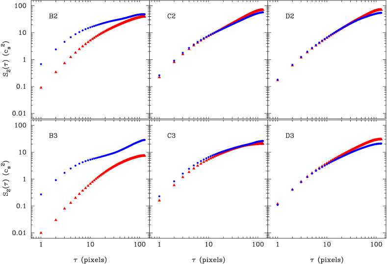
Figure 1: The second order velocity structure function, $S_{2}(\tau)$, along axes parallel (red triangles) and perpendicular (blue circles) to the mean magnetic field direction for velocity fields from turbulent simulations. Velocity anisotropy is evident in the strong field model cases (B2, B3) as a larger scaling amplitude and shallower index for the structure function perpendicular to the mean field direction.

where $\tau=\tau_{\parallel}\mathbf{e_{\parallel}}+\tau_{\perp}\mathbf{e_{\perp}}$; $\mathbf{e_{\parallel}},\mathbf{e_{\perp}}$ are unit vectors parallel and perpendicular respectively to the local mean magnetic field direction, and the angle brackets denote a spatial average over the volume (Cho, Lazarian, & Vishniac 2002). Here, we restrict our analysis to the projected plane appropriate for the velocity field to facilitate comparison with model observations in §3.2. In this case, the $v_{2}$ component projects into the plane defined by axes 1 and 3. Figure 1 shows the 2nd order structure functions, $S_{2}(0,\tau_{\perp})$ and $S_{2}(\tau_{\parallel},0)$. Power laws are fit over the pixel range 5-15 to exclude the steep component at small scales that results from grid-scale numerical dissipation of the simulation. The amplitudes and spectral indices of an equivalent, first order structure function, $(S_{2})^{1/2}$, are listed in Table 2. Velocity anisotropy is clearly identified in the B2 and B3 simulation snapshots as the slope and amplitude of the orthogonal structure functions are different. For the intermediate (snapshots C2,C3) and weak (snapshots D2,D3) B-field cases, the structure functions are statistically equivalent, indicative of globally isotropic velocity fields with slopes ($\sim$0.5) that are typical of strongly supersonic, super-Alfvenic turbulent flows. The absence of velocity anisotropy results from the local distortions of the magnetic field that dilute any signature to large scale anisotropy.

3.2 Model Spectroscopic Data Cubes

Observers do not directly recover the 3 dimensional velocity fields. Wide field spectroscopic imaging measures line intensity as a function of position on the sky and velocity along an axis. The precise shape of a line profile is dependent on density, the projected velocity component, temperature, and chemical abundance that are integrated along the line of sight and affected by line excitation and opacity. To place the model velocity and density fields from the computational simulations in the same domain as observations, we generate synthetic line profiles of ¹²CO and ¹³CO  J=1-0 emission. Details of the line excitation and radiative transfer calculations are described by Brunt & Heyer (2002). The assumed abundance values of ¹²CO and ¹³CO  relative to ${\rm H}_{2}$  are 1.0$\times$10^-4 and 1.25$\times$10^-6 respectively. We adopt a uniform kinetic temperature of 15 K, which corresponds to a one dimensional sound speed of 0.22 km s^-1. The adopted mean volume density of ${\rm H}_{2}$  is $n=1000$ cm^-3.

The choice of constructing synthetic profiles of the high opacity ¹²CO  emission is motivated by two factors. First, the ¹²CO J=1-0 line is the most common tracer of cloud structure so there are many observational data sets available to compare with these models. To be sure, ¹²CO does not effectively probe the high density cores of molecular clouds where star formation takes place. However, these regions comprise a small fraction of the cloud mass and volume (Heyer, Ladd, & Carpenter 1996; Goldsmith etal 2008). Brunt & Heyer (2002) examined the effects of line opacity on the gas dynamics perceived by observations. With the exception of micro-turbulent velocity fields, they found that ¹²CO measurements reliably recover the velocity field statistics. Although the local optical depth can be large within a volume, the macro-turbulent velocity fields provide an effective large velocity gradient condition that allows most photons from the surface of the local volume to escape. In addition, owing to radiative trapping, ¹²CO is detected over a broader area than the lower opacity lines so there are simply more measurements and information on the largest scales. Nevertheless, to re-examine the effects of line opacity, we also generate and analyze synthetic profiles of the ¹³CO  J=1-0 transition.

3.3 Axis-Constrained PCA Applied to Model Data Cubes

The utility of the analysis described in $\S$2 is assessed by its application to the synthetic ¹²CO  and ¹³CO  data cubes constructed from the MHD model density and velocity fields. Does the analysis recover velocity anisotropy when this is present in the raw velocity field, for the case of strong magnetic fields? Does the method verify isotropic velocity fields in the intermediate and weak field cases?

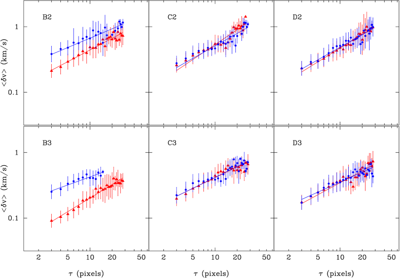
Figure 2: The axis-constrained PCA $<\delta v>,\tau$ relationships derived from synthetic spectroscopic data cubes of ¹²CO J=1-0 emission for the $x$ axis ( along the mean magnetic field; red triangles) and $y$ axis ( perpendicular to the mean magnetic field; blue circles). The error bars reflect the standard deviation of values within each 1 pixel wide bin of $\tau$. The method recovers the anisotropy intrinsic to the B2 and B3 model velocity fields and verifies the isotropic velocity fields of the intermediate (C2,C3) and weak field (D2,D3) models.

Here, we examine the synthetic spectroscopic data cubes derived from the $v_{2}$ velocity field for position angle $\theta$=90^∘, i.e. corresponding to alignment of the $x$-axis with the mean magnetic field direction in the plane of the sky. The results of the axis-constrained PCA method (with $\Delta$=2), as applied to all model snapshots, are shown in Figure 2. Magnetically aligned anisotropy is clearly identified for the B2 and B3 simulation snapshots as a separation of the set of points $(<{\delta}v>,\tau)$ derived respectively along the $x$ and $y$ axes of the model data cubes. This separation of points is qualitatively similar to the corresponding true structure functions calculated directly from the velocity fields that are shown in Figure 1. For the intermediate- (C2,C3) and weak- (D2,D3) magnetic field snapshots, there is a strong overlap of points $(<{\delta}v>,\tau)$ derived for the orthogonal axes. This indicates velocity isotropy with respect to the mean magnetic field, and is in agreement with the true velocity structure functions for the models.

To assess the method quantitatively, bisector fits of power laws with parameters, $\alpha$, $v_{\circ}$, are fit to each set of points for each axis over the range $3\leq\tau\leq 30$ pixels. The scaling exponents, $\gamma_{\parallel}$ and $\gamma_{\perp}$, of the structure function are derived from the fitted parameters, $\alpha_{\parallel}$ and $\alpha_{\perp}$, according to equation 10. The results for the ¹²CO and ¹³CO  model data cubes are summarized in Table 3. With the exception of the C3 model data cube, there are no significant differences between the power law parameters derived from ¹²CO and ¹³CO  model cubes, demonstrating that opacity effects do not significantly skew the derived velocity field statistics.

For the strong field simulations, the separation of points in Figure 2 is due to a combination of a larger normalization constant and shallower index for the perpendicular structure function. Moreover, the anisotropy is stronger in the later stage simulation (comparing B3 with B2). There are, however, discrepancies between the values of $\gamma$ determined directly from the velocity field in Table 2 and those determined by PCA that are listed in Table 3. The root-mean-square difference between power law indices is 0.12 (23%). This discrepancy is due in part, to the difficulty in measuring a power law index of structure functions of velocity fields produced by the computational simulations that have limited inertial range (Vestuto, Ostriker, & Stone 2003). In addition, the PCA eigenprojection along a single axis tends to limit the dynamic range of spatial scales over which the power laws parameters are derived. Despite this discrepancy of the scaling exponents, these results demonstrate the ability of the axis constrained PCA eigenfunctions to show a clear signature of velocity anisotropy induced by MHD turbulence.

4 The Taurus Molecular Cloud

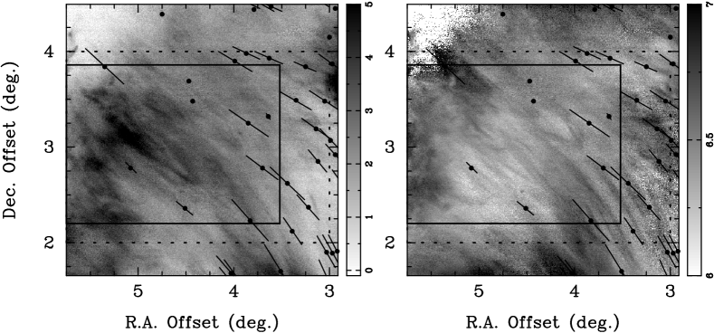
Figure 3: (left) Image of ¹²CO J=1-0 emission of a sub-field within the Taurus molecular cloud integrated over the velocity interval 5.5 to 7.5 km s^-1 and (right) image of ¹²CO velocity centroid (Narayanan etal 2008), with overlay of optical polarization vectors from the compilation by Heiles (2000). The molecular line emission and velocities exhibit streaks that are aligned along the local magnetic field direction. The solid line box outlines the area upon which the axis constrained PCA method is applied. The dotted line box shows the area within which the polarization angles are averaged to esimate the mean magnetic field direction.

The Taurus Molecular Cloud provides a valuable platform to investigate interstellar gas dynamics and the star formation process, owing to its proximity (140 pc) and the wealth of complementary data. Narayanan etal (2008) present new wide-field imaging observations of ¹²CO and ¹³CO  J=1-0 emission from the central 100 deg² of the Taurus cloud complex, obtained with the FCRAO 14m telescope. The images identify a low column density substrate of gas that contain subtle streaks of elevated ¹²CO emission aligned along the local magnetic field direction as determined from stellar polarization measurements (Heiles 2000). Images of ¹²CO J=1-0 integrated intensity and centroid velocity with measured polarization vectors from this subfield are shown in Figure 3. These show a connection between the density and velocity fields. While the origin of these streaks is unknown, their rigorous alignment with the polarization vectors strongly suggests that the interstellar magnetic field plays a prominent role in the gas dynamics of this low density material.

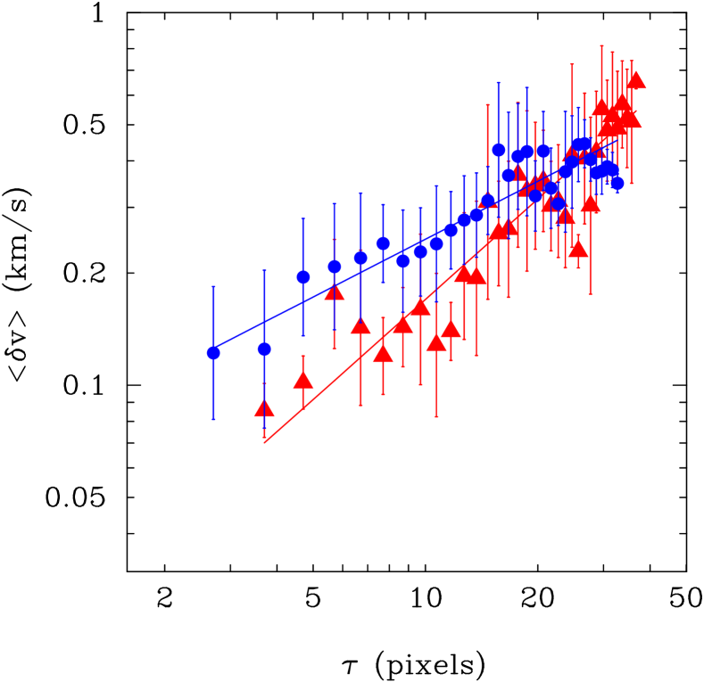
Figure 5: The PCA derived $\delta v,\tau$ relationship derived from the ¹²CO spectroscopic data cube of the Taurus sub-field rotated to align the x-axis with the angle of maximum anisotropy, $\theta_{MAX}=46^{\circ}$. The red triangles are points derived along the rotated x-axis and the blue circles are points derived along the rotated y-axis. The error bars reflect the standard deviation of values in each bin. The pattern is similar to that found from the B2, B3 simulation snapshots in Figure 2 and suggests an important role of the magnetic field on the local gas dynamics.

To assess the degree of velocity anisotropy within this sub-region of the Taurus molecular cloud, we have applied the axis constrained PCA method to the ¹²CO data from this imaging survey. The precise field is described by the solid box in Figure 3. We do not consider the ¹³CO  J=1-0 data since the signal is weak from this low column density sector of the cloud. The mean, local polarization angle, derived from 16 measurements within the field is 52${}^{\circ}\pm$10^∘. Assuming the polarization is induced by selective absorption of background starlight by magnetically aligned, elongated dust grains, this angle corresponds to the local magnetic field direction (Purcell 1979; Draine 2003). Figure 4 shows the variation of the anisotropy indices, $\Psi_{1}$ and $\Psi_{2}$, with position angle (measured east of north) for ¹²CO data within this subfield of the Taurus cloud. For $\Psi_{1}$, which considers the differences in scaling exponents, the fitted parameters are $\Psi_{\circ}$=0.49$\pm$0.03 and $\theta_{MAX}$=41${}^{\circ}\pm$2^∘. For $\Psi_{2}$, which measures anisotropy based on the differences of the normalization constants, $\Psi_{\circ}$=0.56$\pm$0.03 and $\theta_{MAX}$=46${}^{\circ}\pm$2^∘. The angle of maximum anisotropy is within 6-11^∘ of the local magnetic field direction and the mean position angle of the emission streaks of ¹²CO emission. The $x$ and $y$-axis structure functions derived at $\theta_{MAX}$=46^∘ are shown in Figure 5. These distributions show the same pattern of offsets between the parallel and perpendicular structure functions measured in the strong field simulation snapshots (B2,B3) shown in Figure 2. For the Taurus field, the power law index of the structure function derived from ¹²CO along the $x$-axis (i.e. the direction aligned with the polarization) is steeper (0.81$\pm$0.05) than the index of the $y$-axis structure function (0.34$\pm$0.06). The steeper power law along the x-axis is indicative of a velocity field more dominated by large scales. Similar to the model structure functions in the strong magnetic field cases, the normalization of the $y$-axis structure function, $v_{\circ,y}$ is 0.08 km s^-1 and larger than the value of the $x$-axis structure function ($v_{\circ,x}$=0.02 km s^-1). Thus, the smooth variation of density along the presumed magnetic field is mirrored by a smooth variation in the velocity, and the stronger variation in density in the perpendicular direction (streakiness) is mirrored by a stronger variation in the velocity. Indeed, preliminary analysis shows that in the direction perpendicular to the projected magnetic field, displacements between the peaks in integrated intensity and velocity centroids are similar with typical values 0.2 to 0.4 pc.

The results shown in Figures 3,4,5 are suggestive of velocity anisotropy induced by strong MHD turbulence, as described by GS95 and verified by computational simulations (Cho, Lazarian, & Vishniac 2002; Vestuto, Ostriker, & Stone 2003). We note that the observed spectral slope parallel to the field, $\gamma_{\parallel}$, is steeper than the value predicted for incompressible MHD turbulence by GS95 but is similar to values derived for the strong field (B2, B3) simulations. Velocity anisotropy could be produced by processes other than MHD turbulence. A systematic flow of material that is “channeled” by the magnetic field may also generate differences in the parallel and perpendicular structure functions. Such large scale gradients would produce steep spectral indices ($\gamma\geq 1$). However, the observed high frequency variation of velocities perpendicular to the field are not characteristic of such large scale shear flows. Regardless of its origin, the near alignment of the velocity anisotropy with the local magnetic field direction demonstrates the importance of the interstellar magnetic field on the gas dynamics within this low density component of the Taurus molecular cloud.

4.1 The Magnetic Field Strength in the Taurus Cloud Envelope

Since anisotropy is only evident in models with strong magnetic fields, the identification of such anisotropy within observational data offers a proxy measure of the magnetic field and its effect upon the neutral gas (Vesuto, Ostriker, & Stone 2003). Specifically, the amplitude of the mean magnetic field, $B_{\circ}=|\langle{\bf B}\rangle|=c_{s}\sqrt{4{\pi}{\rho}/\beta}$, may be estimated from values of $\beta$ that are constrained by the observations. The measured degree of velocity anisotropy is sensitive to the projected component of the mean field in the plane of the sky. It is improbable that the magnetic field threading an interstellar cloud is aligned in the sky plane. Therefore, measures of velocity anisotropy provide a lower limit to the value of $B_{\circ}$.

Based on our analyses, the anisotropy measured in the Taurus subfield is not as large as in the strong field snapshots (B2,B3), but it is larger than the anisotropy limits for the intermediate-field strength model snapshots (C2,C3). Given this bracketing, we can assign an approximate value of $\beta$=0.03 to the Taurus subfield as a logarithmic midpoint between the intermediate and strong field models. Since the observed region is within the low column density regime of the Taurus Cloud, we set the kinetic temperature to be 15 K and the mean density to be 250 cm^-3. These values for the temperature and density are reasonably constrained by non-LTE excitation models that match the observed ¹²CO and ¹³CO  J=1-0 intensities from the sub-thermally excited component of the Taurus cloud (Goldsmith etal 2008). The magnetic field strength corresponding to these values of $\beta$, kinetic temperature, and gas density is 14 $\mu$G. As noted above, this is a lower limit on the total magnetic field strength since the velocity anisotropy is not sensitive to the line-of-sight component of the magnetic field.

Zeeman measurements of the OH line emission from the L1544 dark cloud, located $\sim$4 degrees to the south-west of the subfield in Taurus, identify a line of sight field strength of 11 $\mu$G (Crutcher & Troland 2000). While this value is comparable to our coarse estimate of the field, these OH Zeeman observations are toward higher column density material ($N(H_{2})\sim 2\times 10^{22}$) than is likely present in the Taurus subfield. If this higher column density reflects a larger volume density and if the magnetic field is correspondingly compressed, the field in the diffuse parts of the Taurus cloud may be smaller.

The Chandrasekhar & Fermi (1953) method offers an additional measure of the magnetic field strength in interstellar clouds. It attributes deviations of the local magnetic field from the mean field direction to linear-amplitude transverse MHD waves such that

$$({\delta}B/B_{p})=|{\delta}v|/v_{A}$$ (15)

where $B_{p}$ is the projection of the mean magnetic field on the plane of the sky, ${\delta}B$ and $|{\delta}v|$ are components of the magnetic and velocity perturbations transverse to $B_{p}$, and $v_{A}$ is the Alfvén velocity. Assuming polarization vectors accurately track the local magnetic field direction and transverse velocity perturbations in the two directions perpendicular to $\hat{B}$ are comparable, the Chandrasekhar-Fermi method is rewritten in terms of observational measures,

$$\sigma_{pol}=f(4\pi\rho_{\circ})^{1/2}\sigma_{v}/B_{p}$$ (16)

where $\sigma_{pol}$ is the dispersion of polarization angles measured in radians, $\sigma_{v}$ is the line of sight velocity dispersion, $\rho_{\circ}$ is the mean density of the gas, and the factor, f, accounts for density inhomogeneity and line of sight integration. Ostriker, Stone, & Gammie (2001) and Padoan etal (2001) determine $f\approx$0.4-0.5 from computational simulations. The dispersion of measured optical polarization angles within the target field is 0.17 radians. The line of sight velocity dispersion determined from the ¹³CO  data is 0.38 km s^-1. Assuming a mean density of 250 cm^-3 and f=0.5, the derived mean field strength is 14 ${\mu}G$. Thus, our PCA-based estimate of the magnetic field strength in Taurus also compares favorably to the value derived by the Chandrasekhar-Fermi method.

4.2 The Magnetic Support of the Taurus Cloud Envelope

The degree to which the magnetic field can support a volume against self-gravitational collapse is parameterized by the mass to flux ratio with respect to the critical value, $(M/\Phi)_{crit}=0.16/G^{1/2}$ (Nakano & Nakamura 1978). The magnetic critical index, $\mu$, is the ratio of the mass to flux ratio of a volume to this critical value,

$$\mu=(M/\Phi)/(M/\Phi)_{crit}=7.6\times 10^{-21}N(H_{2})/B$$ (17)

where $N(H_{2})$ is the gas column density in cm^-2 along field lines and B is the magnetic field strength expressed in $\mu$G. Owing to projections of the magnetic field and the mass distribution along field lines, the observed index, $\mu_{obs}$, overestimates the true magnetic index. Assuming random orientations of the magnetic field and flattened gas distribution with respect to the observer, one can derive a statistical correction to the observed value, $<\mu>=\mu_{obs}/3$ to assess whether a volume is super-critical ($<\mu>$ greater than 1) or sub-critical ($<\mu>$ less than 1) (Heiles & Crutcher 2005).

Goldsmith etal (2008) derive the distribution of molecular hydrogen over 100 deg² of the Taurus Molecular Cloud using the ¹²CO and ¹³CO  J=1-0 data of Narayanan etal (2008). From the Goldsmith etal (2008) image, the mean column density within the Taurus subfield analyzed in this study is 1.5$\times$10²¹ cm^-2. For a magnetic field with strength 14 $\mu$G, this column density corresponds to an observed magnetic index of $\mu_{obs}=0.81$. Applying the statistical correction for projections, $<\mu>=0.27$. This low column density subfield within the Taurus cloud is magnetically sub-critical indicative of a magnetically supported cloud envelope. Such sub-critical, low column density envelopes are expected given the exposure to the ambient UV radiation field that maintains a sufficient degree of ionization to couple the neutral material to ions. The ambipolar diffusion time scale is long with respect to the dynamical time of the envelope. While star formation within the high density cores and filaments of the Taurus cloud attest to the gravitational collapse and lack of magnetic support within localized regions, these occupy a small fraction of the mass and area of the cloud. Goldsmith etal (2008) report that 50% of the mass and 75% of the area of Taurus have molecular column densities less than 2$\times$10²¹ cm^-2. If this column density regime is similar to the subfield analyzed in this study, then the Taurus molecular cloud envelope remains magnetically supported.

5 Summary

We have developed an analysis method to assess velocity anisotropy within interstellar molecular clouds from spectroscopic imaging observations. Such anisotropy is predicted from theory of strong MHD turbulence (GS95). The utility of our method is demonstrated using MHD simulations with varying magnetic field strengths. Velocity anisotropy is recovered in models with strong magnetic fields ($\beta=0.01$) oriented perpendicular to the line-of-sight. No anisotropy is measured in simulations with the magnetic field pressure more comparable to the local thermal pressure, or a few times larger ($\beta=1.0,0.1$). The analysis is applied to ¹²CO J=1-0 emission from a low density sub-region within the Taurus molecular cloud. We detect velocity anisotropy that is aligned within $\sim$10 degrees of the local magnetic field direction. This coincidence of the field direction with measured anisotropy in small-scale velocity variations demonstrates a strong coupling of the interstellar field with the neutral gas that may result from MHD turbulent flows. Our estimate of the plane-of-sky magnetic field strength based on our velocity anisotropy analysis is in agreement with the value derived using the Chandrasekhar-Fermi method. Based on our estimated magnetic field strength combined with column density measurements, we find that the low-density envelope of Taurus, which comprises the bulk of the cloud’s mass, is magnetically subcritical.

Table 1: MHD Simulation Parameters

Model	$\beta$	$t/t_{s}$	$M_{s}$
B2	0.01	0.07	7.4
C2	0.10	0.04	7.6
D2	1.00	0.05	7.2
B3	0.01	0.19	4.9
C3	0.10	0.09	4.9
D3	1.00	0.09	4.9

Table 2: Structure Function Parameters: $(S_{2}(\tau))^{1/2}=v_{\circ}\tau^{\gamma}$

Model	$\gamma_{\parallel}$	$\gamma_{\perp}$	$v_{\circ,\parallel}$	$v_{\circ,\perp}$
B2	0.68	0.35	0.47	1.76
C2	0.53	0.49	0.80	0.89
D2	0.63	0.61	0.60	0.63
B3	0.82	0.29	0.14	1.16
C3	0.49	0.44	0.74	0.92
D3	0.56	0.52	0.54	0.57

Table 3: Structure Function Parameters Derived from Model Data Cubes

	12CO				13CO
Model	$\gamma_{\parallel}$	$\gamma_{\perp}$	$v_{\circ,\parallel}$	$v_{\circ,\perp}$	$\gamma_{\parallel}$	$\gamma_{\perp}$	$v_{\circ,\parallel}$	$v_{\circ,\perp}$
B2	0.46	0.26	0.11	0.23	0.55	0.32	0.08	0.15
C2	0.67	0.53	0.09	0.12	0.57	0.44	0.10	0.12
D2	0.62	0.53	0.10	0.11	0.53	0.59	0.10	0.10
B3	0.61	0.15	0.04	0.17	0.62	0.23	0.04	0.13
C3	0.38	0.39	0.12	0.12	0.34	0.53	0.10	0.08
D3	0.49	0.31	0.09	0.11	0.61	0.41	0.07	0.09

Figure 4: The variation of the anisotropy indices, $\Psi_{1}$ (left) and $\Psi_{2}$ (right), with position angle, $\theta$. For each index, the solid line shows the fit of equation 13 to the set of points. The dashed vertical lines show $\langle\theta_{B}\rangle\pm 1\sigma$ inferred from optical polarization measurements of background stars within the subfield. The angle of maximum anisotropy is nearly aligned with the local magnetic field direction, which suggests a relationship between velocity anisotropy and the interstellar magnetic field induced by strong MHD turbulence.

References

- Brunt & Heyer (2002) Brunt, C.M., & Heyer, M.H. 2002, ApJ, 566,289
- Brunt etal (2003) Brunt, C.M., Heyer, M.H., Vazquez-Semadeni, E. & Pichardo, B. 2003, ApJ, 595, 824
- Brunt (2003) Brunt, C.M. 2003, ApJ, 584, 293
- (4) Brunt, C.M., & Mac Low, M. 2004, ApJ, 604, 196
- Chandrasekhar & Fermi (1954) Chandrasekhar, S. & Fermi, E. 1953, ApJ, 118, 113
- (6) Cho,J., Lazarian, A., & Vishniac, E.T. 2002, ApJ, 564, 291
- (7) Crutcher, R.M. & Troland, T.H. 2000, ApJ, 537, L139
- (8) Draine, B.T. 1979, ARA&A, 41, 241
- (9) Goldreich, P. & Sridhar, S. 1995, ApJ, 438, 763
- (10) Goldsmith, P.F., Heyer, M.H., Narayanan, G., Snell, R.L., Li, D., & Brunt, C.M. 2008, submitted to ApJ
- (11) Heiles, C. 2000, AJ, 119, 923
- (12) Heiles, C. & Crutcher, R. 2005, in Cosmic Magnetic Fields, eds. R. Wielebinski & R. Beck (Springer: Berlin), p 137
- (13) Heyer, M.H., Ladd, E.L., & Carpenter, J.M. 1996, ApJ, 463, 630
- (14) Heyer, M.H., & Schloerb, F.P. 1997, ApJ, 475, 173
- (15) Heyer, M.H., & Brunt, C.M. 2004, ApJ, 615, L45
- (16) Lizano, S. & Shu, F.H. 1989, ApJ, 342, 834
- (17) Maron, J. & Goldreich, P. 2001, ApJ, 554, 1175
- (18) Mouschovias, T.C. 1976, ApJ, 207, 141
- (19) Nakano, T. & Nakamura, T, 1978, PASJ, 30, 671
- (20) Ossenkopf, V., Esquivel, A., Lazarian, A., & Stutzki, J. 2006, AA, 452, 2230
- (21) Ostriker, E.C., Stone, J.M., & Gammie, C.F. 2001, ApJ, 546, 980
- (22) Narayanan, G., Heyer, M.H., Brunt, C.M., Goldsmith, P.F., Snell, R.L., & Li, D. 2008, submitted to ApJ
- (23) Padoan, P. Goodman, A. Draine, B.T., Juvela, M., Nordlund, A. Rognvaldsson, O.E. 2001, ApJ, 559, 1005
- (24) Purcell, E.M. 1979, ApJ, 231, 404
- (25) Vazquez-Semadeni, E., Kim, J., & Ballesteros-Paredes, J. 2005, ApJ, 630, L49
- (26) Vestuto, J.G., Ostriker, E.C., & Stone, J.M. 2003, ApJ, 590, 858 ApJ, 590, 858
- (27) Watson, W.D., Wiebe, D.S., McKinney, J.C., & Gammie, C.F. 2004, ApJ, 604, 707
- (28) Wiebe, D.S. & Watson, W.D. 2007, ApJ, 655, 275