Hyperspherical Partial Wave Theory with Two-term Error Correction

Abstract

Hyperspherical Partial Wave Theory has been applied to calculate T-matrix elements and Single Differential Cross-Section (SDCS) results for electron-hydrogen ionization process within Temkin-Poet model potential. We considered three different values of step length to compute the radial part of final state wave function. Numerical outcomes show that T-matrix elements and SDCS values depend on the step length h. Here, we have presented T-matrix elements and the corresponding SDCS results for 0.0075 a.u., 0.009 a.u. and 0.01 a.u. values of h and for 27.2eV, 40.8ev and 54.4eV impact energies. With the help of the calculated data for three different step lengths, we have been able to evaluate a two-term error function depending on the step length h. Finally, two-term error corrected T-matrix elements and the corresponding SDCS values have been computed. We fitted our two-term error corrected SDCS results by a suitable curve and compared with the benchmark results of Jones et al. [Phys. Rev. A, 66, 032717 (2002)]. Our fitted curves agree very well with the calculated results of Jones et al. and two-term error corrected SDCS results somewhere agree with the benchmark results. Two-term error corrected SDCS results are significantly better than the calculated SDCS results of different step lengths.

I Introduction

The electron-impact ionization of hydrogen probes the correlated quantal dynamics of two electrons moving in the long-range Coulomb field of a third body. As such it remains one of the most fundamental and interesting problems in nonrelativistic quantum mechanics. There are many attempts for a complete solution but all of these face enormous difficulties and have only limited success. Among these the most successful attempts are the method of Convergent Close-Coupling (CCC) and Exterior Complex Scaling (ECS). Another promising approach for the electron-hydrogen atom ionization problem is the Hyperspherical Partial Wave (HPW) approach. After the successful applications of HPW theory to compute triple differential equal-energy-sharing cross-section results A1 ; A2 ; A3 ; A4 ; A5 ; A6 , we aspire to calculate SDCS results. Before considering the full electron-hydrogen ionization problem, here, we consider Coulomb three-body system within Temkin-Poet (TP) model B1 ; B2 . The TP model of electron-hydrogen collision is now widely considered as an ideal testing ground for the improvement of general methods intended for full Coulomb three-body problem. In this context, the calculated SDCS results of other theories for TP model potential are praiseworthy. Among these the attempt of Jones et al. C1 ; C2 is remarkable, they obtained benchmark results. They have developed a variable-spacing finite-difference algorithm that rapidly propagates the general solution of Schrödinger equation to large distances, originally used by Poet D to solve TP model. The ECS calculation is generally in good agreement with the benchmark results of Jones et al. except at the extreme asymmetric energy sharing D2 . The calculated singlet SDCS curves of CCC method are wavy, Bray considered a smooth curve by educated guess E . The CCC results agree nicely with benchmark results of Jones et al. only for the triplet case (generally, CCC does not yield convergent amplitude for the triplet case, except for total angular momentum zero). We also note the work of Miyashita et al. F . They have presented SDCS for total energy of 4Ry, 2Ry and 0.1Ry using two different methods. One produces an asymmetric energy distribution similar to that of CCC while the other gives a symmetric distribution. Both contain oscillations. It should be noted that recently, we have used HPW approach to calculate SDCS results for full electron-hydrogen-ionization problem at 60eV incident energy G . The resultant curve was wavy and calculated cross-section results are irrelevant at extreme energy sharing. We had fitted our calculated SDCS data by a fourth order parabola and compared with the experimental values of Shyn H . Our fitted curve agrees excellently with experimental results. In this article we present the SDCS results for TP model using HPW method with two-term error correction. Here, we introduce a procedure to calculate error function. The results are obtained for intermediate (27.2eV, 40.8eV and 54.4eV) energies. We have calculated T-matrix elements and the corresponding SDCS data for three different values of step length h (0.0075 a.u., 0.009 a.u. and 0.01 a.u.), use to calculate radial part of final state wave function numerically. Numerical observation shows that the T-matrix elements depend on h. Using the data for various step lengths, we calculated two-term error function, depends on h. Finally, two-term error corrected SDCS values were computed. The nature of error corrected SDCS undulating curves suggests a fit, with a proper function. HPW method for TP model is reproduced in Sec.II, procedure of calculation is presented in Sec. III, two-term error correction process is given in Sec. IV, results are presented in Sec. V with a short discussion, and some concluding remarks are found in Sec. VI. Atomic units are used throughout this paper except where otherwise noted.

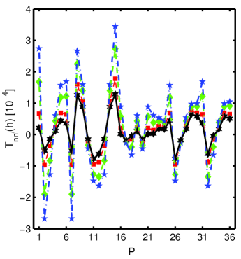
Figure 1: (Color online) The values of $T_{nn^{\prime}}^{0}$ (zero indicates singlet) for three different step lengths at 27.2eV incident electron energy. Square points for h = 0.0075, diamond points for h = 0.009 and pentagon points for h = 0.01. Hexagon points represent the values of $T_{nn^{\prime}}^{0*(2)}$ at the same energy.

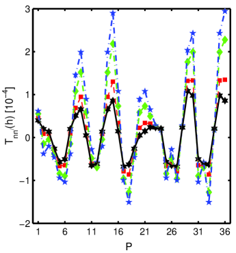
Figure 2: (Color online) Same as in Fig. 1 but for triplet case.

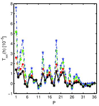
Figure 3: (Color online) Same as in Fig. 1 but for 40.8eV incident electron energy.

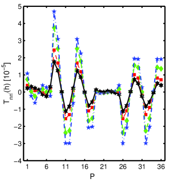
Figure 4: (Color online) Same as in Fig. 3 but for triplet case.

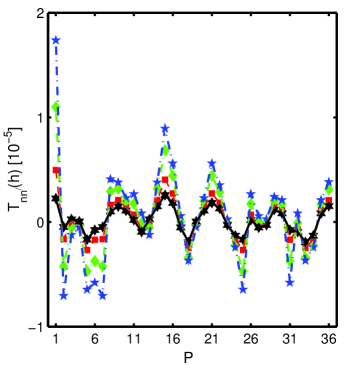
Figure 5: (Color online) Same as in Fig. 1 but for 54.4eV incident electron energy.

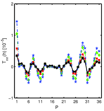
Figure 6: (Color online) Same as in Fig. 5 but for triplet case.

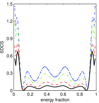
Figure 7: (Color online) Singlet SDCS ($\pi a_{0}^{2}/Ry$) vs the energy fraction $E_{b}/E$ for three different step lengths and for $T_{nn^{\prime}}^{0*(2)}$ elements at 27.2eV impact electron energy. Continuous curve, $T_{nn^{\prime}}^{0*(2)}$ elements; dashed curve, for h = 0.0075 a.u.; dash-dotted curve, for h = 0.009 a.u.; dash-double dotted curve, for h = 0.01 a.u..

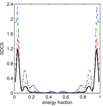
Figure 8: (Color online) Triplet SDCS ($\pi a_{0}^{2}/Ry$) vs the energy fraction $E_{b}/E$ for three different step lengths and for $T_{nn^{\prime}}^{1*(2)}$ elements at 27.2eV impact electron energy. Continuous curve, $T_{nn^{\prime}}^{1*(2)}$ elements; dashed curve, for h = 0.0075 a.u.; dash-dotted curve, for h = 0.009 a.u.; dash-double dotted curve, for h = 0.01 a.u..

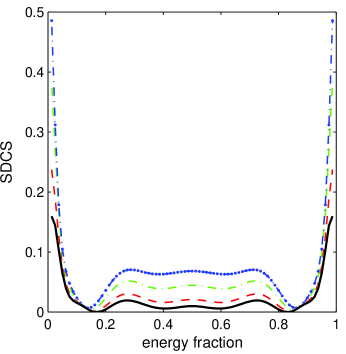
Figure 9: (Color online) Same as Fig. 7 for 40.8eV.

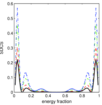
Figure 10: (Color online) Same as Fig. 8 for 40.8eV.

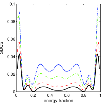
Figure 11: (Color online) Same as Fig. 7 for 54.4eV.

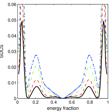
Figure 12: (Color online) Same as Fig. 8 for 54.4eV.

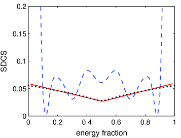
Figure 13: (Color online) Singlet SDCS ($\pi a_{0}^{2}/Ry$) vs the energy fraction $E_{b}/E$ for incident energy 27.2eV. Continuous curve, fitted function; dashed curve, present results corresponding $T_{nn^{\prime}}^{0*(2)}$ elements; dotted curve, calculated results of Jones et al. C2 .

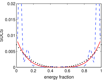
Figure 14: (Color online) Triplet SDCS ($\pi a_{0}^{2}/Ry$) vs the energy fraction $E_{b}/E$ for incident energy 27.2eV. Continuous curve, fitted function; dashed curve, present results corresponding $T_{nn^{\prime}}^{1*(2)}$ elements; dotted curve, calculated results of Jones et al. C2 .

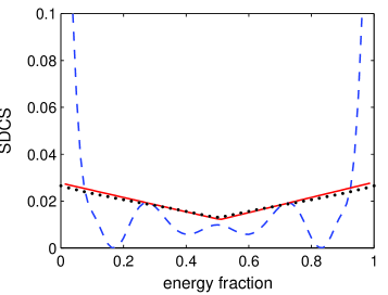
Figure 15: (Color online) Same as Fig. 13 for 40.8eV.

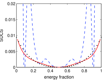
Figure 16: (Color online) Same as Fig. 14 for 40.8eV.

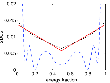
Figure 17: (Color online) Same as Fig. 13 for 54.4eV.

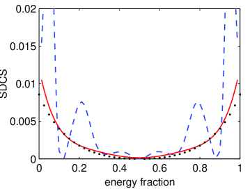
Figure 18: (Color online) Same as Fig. 14 for 54.4eV.

II Theory

The T-matrix element, we use in cross-section calculation, is given by

$$T_{fi}^{s}=<\Psi_{fs}^{(-)}|V_{i}|\Phi_{i}>.$$ (1)

In this expression $\Phi_{i}$ is the unperturbed initial channel wave function, satisfying certain exact boundary condition at large distance and $V_{i}$ is the corresponding perturbation potential. Here, $\Psi_{fs}^{(-)}$ is the symmetrized scattering state (see Newton N31 for definition). For information regarding electron-hydrogen-ionization within TP model potential, one may solve the corresponding Schrödinger equation. We start by writing the Schrödinger equation for the full electron-hydrogen ionization problem

$$\Big{[}-\frac{1}{2}\nabla_{\vec{r_{1}}}^{2}--\frac{1}{2}\nabla_{\vec{r_{2}}}^{2}-\frac{1}{r_{1}}-\frac{1}{r_{1}}+V_{12}\Big{]}\Psi_{fs}^{(-)}=E\Psi_{fs}^{(-)}$$ (2)

where

$$V_{12}=\frac{1}{|\vec{r_{1}}-\vec{r_{2}}|}.$$ (3)

To calculate the final channel symmetrized continuum state $\Psi_{fs}^{(-)}$ we use hyperspherical coordinate $R=\sqrt{r_{1}^{2}+r_{2}^{2}}$, $\alpha=arctan(r_{2}/r_{1})$, $\hat{r_{1}}=(\theta_{1},\phi_{1})$, $\hat{r_{2}}=(\theta_{2},\phi_{2})$ and $\omega=(\alpha,\hat{r_{1}},\hat{r_{2}})$. Also we set $P=\sqrt{p_{1}^{2}+p_{2}^{2}}$, $\alpha_{0}=arctan(p_{2}/p_{1})$, $\hat{p_{1}}=(\theta_{p_{1}},\phi_{p_{1}})$, $\hat{p_{2}}=(\theta_{p_{2}},\phi_{p_{2}})$ and $\omega_{0}=(\alpha_{0},\hat{p_{1}},\hat{p_{2}})$ where $\vec{r_{i}}$ and $\vec{p_{i}}$ (i = 1, 2) are the coordinates and momenta of i th charged particles. $\Psi_{fs}^{(-)}$ is then expanded in symmetrized hyperspherical harmonics A1 that are functions of five angular variables and $l_{1},l_{2},n,L,M$, which are, respectively, the angular momenta of two electrons, the order of the Jacobi polynomial in hyperspherical harmonics, the total angular momentum and its projection. For a given symmetry s (s = 0 for singlet and s = 1 for triplet), we decompose the final state as

$$\Psi_{fs}^{(-)}=\sqrt{\frac{2}{\pi}}\sum_{\mu}\frac{F_{\mu}^{s}(\rho)}{\rho^{5/2}}\phi_{\mu}^{s}(\omega)$$ (4)

where $\mu$ is the composite index ($l_{1},l_{2},n,L,M$) and $\rho=PR$ and $\phi_{\mu}^{s}(\omega)$ are orthogonal functions that are product of Jacobi polynomial $P_{l_{1}l_{2}}^{n}$ and coupled angular momentum eigenfunction $Y_{l_{1}l_{2}}^{LM}(\hat{r_{1}},\hat{r_{2}})$ A1 . $F_{\mu}^{s}(\rho)$ then satisfy the infinite coupled differential equations

$$\Big{[}\frac{d^{2}}{d\rho^{2}}+1-\frac{\nu_{\lambda}(\nu_{\lambda}+1)}{\rho^{2}}\Big{]}F_{\mu}^{s}(\rho)+\sum_{\mu^{\prime}}\frac{2\alpha_{\mu\mu^{\prime}}^{s}}{\rho}F_{\mu^{\prime}}^{s}(\rho)=0.$$ (5)

Here $\alpha_{\mu\mu^{\prime}}^{s}$ are the matrix elements of the full three-body interaction potential and $\nu_{\lambda}=\lambda+3/2$ where $\lambda=2n+l_{1}+l_{2}$.

For the cusp model (or TP model) the $V_{12}$ term, derived from the first term of the partial-wave expansion of the electron-electron potential, is given by

$$V_{12}=\frac{1}{r_{>}}=\frac{1}{max(r_{1},r_{2})}.$$ (6)

The TP model calculated in this article is simplification of our earlier calculated full electron-hydrogen problem, and we only consider the case where all angular momenta are zero. Retaining only zero angular momentum terms we have

$$\Psi_{fs}^{(-)}=\sqrt{\frac{2}{\pi}}\sum_{n}\frac{F_{n}^{s}(\rho)}{\rho^{5/2}}\phi_{n}^{s}(\omega)$$ (7)

where $\phi_{n}^{s}=\phi_{(L=l_{1}=l_{2}=0),n}^{s}$. The expression of hyperspherical harmonics where all angular momenta are zero is given by

$$\phi_{(L=l_{1}=l_{2}=0),n}^{s}(\omega)=\frac{1}{2}\Big{\{}1+(-1)^{s+n}\Big{\}}P_{00}^{n}(\alpha)Y_{00}^{00}(\hat{r_{1}},\hat{r_{2}}).$$ (8)

The radial functions $F_{n}^{s}(\rho)$ satisfy an infinite coupled set of equations

$$\Big{[}\frac{d^{2}}{d\rho^{2}}+1-\frac{\nu_{n}(\nu_{n}+1)}{\rho^{2}}\Big{]}F_{n}^{s}(\rho)+\sum_{n^{\prime}}\frac{2\alpha_{nn^{\prime}}^{s}}{\rho}F_{n^{\prime}}^{s}(\rho)=0.$$ (9)

In the above expression

$$\alpha_{nn^{\prime}}^{s}=-<\phi_{n}^{s}|C|\phi_{n^{\prime}}^{s}>/P$$ (10)

and

$$C=-\frac{1}{cos\alpha}-\frac{1}{sin\alpha}+\frac{1}{max(cos\alpha,sin\alpha)}.$$ (11)

Finally, one obtains the T-matrix element in the form (for details see Eqn. (25) of Ref. A1 )

$$T_{fi}^{s}=\sum_{n}C^{s}(n)\phi_{n}^{s}(\omega_{0}).$$ (12)

The modulus square of the T-matrix element, which is used to calculate differential cross-section, is then given by

$$|T_{fi}^{s}|^{2}=\sum_{nn^{\prime}}T_{nn^{\prime}}^{s}\phi_{n}^{s}(\omega_{0})\phi_{n^{\prime}}^{s*}(\omega_{0}).$$ (13)

III Present Calculation

In our present calculation, n, the degree of Jacobi polynomial, was varied from 0 to 11. We considered $n$ = 0, 2, 4, 6, 8, 10 for calculating singlet SDCS results and $n$ = 1, 3, 5, 7, 9, 11 for computing triplet SDCS values N41 . The main numerical task is to calculate the radial functions $F_{n}^{s}(\rho)$ over a wide domain $[0,\infty)$. As earlier A1 , we divide the whole solution interval $[0,\infty)$ into three subintervals $[0,\Delta]$, $(\Delta,R_{0}]$ and $[R_{0},\infty)$, where $\Delta$ has the value of a few atomic unit and $R_{0}$ is the asymptotic matching parameter. $R_{0}$ is needed to be such that $R_{0}\sim 1/\sqrt{E}$, where E is the energy in the final channel A1 . Thus for energies of 27.2eV, 40.8eV and 54.4eV this range parameter $R_{0}$ may be chosen greater than the values 5000 a.u., 3000 a.u. and 2500 a.u., respectively. We have chosen $R_{0}$ around these values in our calculations. For $[R_{0},\infty)$ we have simply analytic solution A1 . We applied a seven-point finite difference scheme A3 for solution in the interval $[0,\Delta]$ with step length h. Now for the difference equations we divided the domain $[0,\Delta]$ into 100 subintervals of length h and $\Delta=100h$. Solution over $(\Delta,R_{0})$ is very simple. Because of the simple structure of equation (9) a Taylor series expansion method with step length 2h works nicely. Presently, we considered three different values of step length h, these are 0.0075 a.u., 0.009 a.u. and 0.01 a.u., respectively. Finally, we calculated $T_{nn^{\prime}}^{s}$ and SDCS results for three different step lengths.

IV Two-term Error Correction

In the previous section, we reproduced the values of $T_{nn^{\prime}}^{s}$ for three different step lengths and observed that $T_{nn^{\prime}}^{s}$ are varied with h. Now, we can consider a relation between $T_{nn^{\prime}}^{s}(h)$ with the error term $E_{nn^{\prime}}^{s}(h)$ as

$$T_{nn^{\prime}}^{s}(h)=T_{nn^{\prime}}^{s*}+E_{nn^{\prime}}^{s}(h)$$ (14)

where $T_{nn^{\prime}}^{s*}$ are the converged results with respect to the step length h. Since in our seven-point finite difference scheme the error term is $Kh^{8}f^{(8)}(\xi)$ A3 where K is a constant and $\xi$ is a linear function of h. The error term of $T_{nn^{\prime}}^{s}(h)$ calculation is $Ch^{8}f^{(8)}(\xi)$ where C is a constant. Instead of $Kh^{8}f^{(8)}(\xi)$, we can write the error term of seven-point finite difference scheme as

$$K_{1}h^{8}f^{(8)}(R_{m})+K_{2}h^{10}f^{(10)}(R_{m})+K_{3}h^{12}f^{(12)}(\xi),$$

for a certain grid point $R_{m}$. Using the above expression, we can easily formulate,

$$E_{nn^{\prime}}^{s}(h)=A_{nn^{\prime}}^{s}h^{8}+B_{nn^{\prime}}^{s}h^{10}+G_{nn^{\prime}}^{s}h^{12}f^{(12)}(\xi)$$ (15)

where $A_{nn^{\prime}}^{s}$, $B_{nn^{\prime}}^{s}$ and $G_{nn^{\prime}}^{s}$ are independent of h. Considering first two terms, we get the expression of two-term error function for $T_{nn^{\prime}}^{s}(h)$ elements

$$E_{nn^{\prime}}^{s(2)}(h)=A_{nn^{\prime}}^{s}h^{8}+B_{nn^{\prime}}^{s}h^{10}.$$ (16)

Corresponding two-term error corrected $T_{nn^{\prime}}^{s*(2)}(h)$ elements satisfy the equation

$$T_{nn^{\prime}}^{s}(h)=T_{nn^{\prime}}^{s*(2)}+E_{nn^{\prime}}^{s(2)}(h).$$ (17)

In the present context, we have considered step lengths of three different values $h_{1}$, $h_{2}$ and $h_{3}$. Therefore, from the equation (17) we have,

$$E_{nn^{\prime}}^{s(2)}(h_{i})-E_{nn^{\prime}}^{s(2)}(h_{j})=T_{nn^{\prime}}^{s}(h_{i})-T_{nn^{\prime}}^{s}(h_{j})$$ (18)

for i, j = 1, 2, 3 and i$\neq$j. The coefficients of $h^{8}$ and $h^{10}$ in the expression (16) are given by

$$A_{nn^{\prime}}^{s} = \frac{(h_{3}^{10}-h_{2}^{10})\{T_{nn^{\prime}}^{s}(h_{2})-T_{nn^{\prime}}^{s}(h_{1})\}-(h_{2}^{10}-h_{1}^{10})\{T_{nn^{\prime}}^{s}(h_{3})-T_{nn^{\prime}}^{s}(h_{2})\}}{(h_{2}^{8}-h_{1}^{8})(h_{3}^{10}-h_{2}^{10})-(h_{3}^{8}-h_{2}^{8})(h_{2}^{10}-h_{1}^{10})}$$

$$B_{nn^{\prime}}^{s} = -\frac{(h_{3}^{8}-h_{2}^{8})\{T_{nn^{\prime}}^{s}(h_{2})-T_{nn^{\prime}}^{s}(h_{1})\}-(h_{2}^{8}-h_{1}^{8})\{T_{nn^{\prime}}^{s}(h_{3})-T_{nn^{\prime}}^{s}(h_{2})\}}{(h_{2}^{8}-h_{1}^{8})(h_{3}^{10}-h_{2}^{10})-(h_{3}^{8}-h_{2}^{8})(h_{2}^{10}-h_{1}^{10})}.$$ (19)

Here we have considered $h_{1}$=0.0075, $h_{2}$=0.009 and $h_{3}$=0.01 so the above expression of $A_{nn^{\prime}}^{s}$ and $B_{nn^{\prime}}^{s}$ reduce to

$$A_{nn^{\prime}}^{s} = 0.05229064077\{T_{nn^{\prime}}^{s}(h_{2})-T_{nn^{\prime}}^{s}(h_{1})\}-0.023472188\{T_{nn^{\prime}}^{s}(h_{3})-T_{nn^{\prime}}^{s}(h_{2})\}$$

$$B_{nn^{\prime}}^{s} = -0.01143107936\{T_{nn^{\prime}}^{s}(h_{2})-T_{nn^{\prime}}^{s}(h_{1})\}+0.006630530581\{T_{nn^{\prime}}^{s}(h_{3})-T_{nn^{\prime}}^{s}(h_{2})\}.$$ (20)

After calculating the $T_{nn^{\prime}}^{s*(2)}$ elements, we have calculated the corresponding two-term error corrected SDCS results.

V Results and Discussion

As we discussed in the section III, we have considered six different values of the degree of Jacobi polynomial. There are total 36 pairs of ($n,n^{\prime}$) in the calculation of $T_{nn^{\prime}}^{s}$. We have labeled those pairs by an integer variable P, varied from 1 to 36. The values of $T_{nn^{\prime}}^{0}$ (zero indicates singlet) for three different step lengths and $T_{nn^{\prime}}^{0*(2)}$ are presented in Fig. 1 for 27.2eV energy, in Fig. 2 for 40.8eV energy and in Fig. 3 for 54.4eV energy. In the Figs. 4, 5, and 6 we have presented the values of $T_{nn^{\prime}}^{1}$ (one indicates triplet) for three different step lengths and $T_{nn^{\prime}}^{1*(2)}$ for energies of 27.2eV, 40.8eV and 54.4eV respectively. Figures show that the magnitudes of $T_{nn^{\prime}}^{s}$ are diminished with the decreasing of the step length. As shown in the figures, the magnitudes of $T_{nn^{\prime}}^{s*(2)}$ are lowest than the values of $T_{nn^{\prime}}^{s}$ for various step length. The curves were drowned joining the points square for h = 0.0075, diamond for h = 0.009, pentagon for h = 0.01 and hexagon for $T_{nn^{\prime}}^{s*(2)}$; show that in the figures, comparatively similar. In our previous calculation primarily to calculate Double Differential Cross-Section (DDCS), SDCS results and somewhere Triple Differential Cross-Section (TDCS) results, we had established good qualitative results. There were significant discrepancies in the magnitude for extreme asymmetric energies. These types of phenomena were happened due to such kind of behavior of $T_{nn^{\prime}}^{s}$ elements, depend tremendously on h. At that time, we drew full electron-hydrogen problem, and it was difficult to envisage the convergence analysis with respect to step length. These figures also show that the calculation of $T_{nn^{\prime}}^{s}$ elements is stable concerning h. The two-term error corrected elements $T_{nn^{\prime}}^{s*(2)}$ are almost less than $T_{nn^{\prime}}^{s}(0.0075)$ and in few cases equal with $T_{nn^{\prime}}^{s}(0.0075)$. This implies that tow-term error correction procedure will be fruitful. In the section, we shall show that the SDCS results for $T_{nn^{\prime}}^{s*(2)}$ elements are significantly better than the SDCS results for h = 0.0075 and other values. In Figs. 7-12, we have compared our calculated SDCS results for three different step lengths and for $T_{nn^{\prime}}^{s*(2)}$ (s = 0 for singlet and s = 1 for triplet) elements. As shown in figures, the SDCS curves are less corrugated and smaller magnitude with the decreasing of step length. The calculated SDCS results for $T_{nn^{\prime}}^{s*(2)}$ elements are smallest in size and least undulating comparison with the SDCS values for three different step lengths. In the case of singlet for 27.2eV and 54.4eV energies, the SDCS results for $T_{nn^{\prime}}^{0*(2)}$ elements are significantly different to that of for three different values of h. At 54.4eV energy, there is an irrelevant peak at equal energy sharing case for h = 0.009 and 0.01. The peak abolished for h = 0.0075 and reduced to a deep for $T_{nn^{\prime}}^{0*(2)}$ elements. For 40.8eV energy, the shape of the curves is approximately same only difference in magnitude. Same things happened in the case of triplet, the scale of curves reduced and wavy nature abolished, as well as singlet. With the change of step lengths, the nature of curves change rapidly, its magnitude reduced and wavy nature abolished swiftly with the modification of the step length, in decreasing order. Magnitude of the curves reduced significantly at the extreme asymptotic region.

VI Compare with Benchmark Results

In this section, we present two-term error corrected results and fitted curves corresponding these values along with the benchmark results of Jones. The oscillating nature of two-term error corrected curves suggests a fit, with a proper function, symmetry about E/2 (E is the energy in the final channel). We looked at the linear-linear function for singlet SDCS values ($y=a+bx+c|x-d|$ where x is the energy of the secondary electron and y is the corresponding singlet SDCS values) and a maximum six degree polynomial for triplet SDCS data ($y=a+bx+cx^{2}+dx^{3}+ex^{4}+fx^{5}+gx^{6}$ where x is the energy of the secondary electron and y is the corresponding triplet SDCS values). For 27.2eV energy, a four degree polynomial proved sufficient for curve fitting. First, we neglected broader data (maximum eight data out of eighty) from the extreme asymptotic region, irrelevant with other data, fitted a function for the rest of the values and drew the fitted curve for the entire energy domain. In Tables 1 and 2, we have presented the coefficients of the fitted curves for three different energies and triplet, singlet cases. Our fitted curves agree very well with the results of Jones. Somewhere, our calculated two-term error corrected results cut and touch the curves of benchmark data. It is very important for HPW approach that our two-term error corrected results are free from any kind of scale, except triplet SDCS results at 27.2eV which have been scaled by a factor of 0.03. In earlier, DDCS and SDCS calculations, we had multiplied our data by a suitable factor for lowering the magnitude and compared with experimental values.

Table 1: Coefficients for fitted curve at various impact energies and triplet case.

Energy	a	b	c	d	e	f	g
27.2eV	0.042012	-0.650385	3.8148108	-10.0556766	10.054884
40.8eV	0.046054	-0.49753	2.90446	-9.505798	16.482738	-14.075808	4.691936
54.4eV	0.0563445	-0.420831	1.529658	-3.071799	3.3675705	-1.874718	0.416538

Table 2: Coefficients for fitted curve at various impact energies and singlet case.

Energy	a	b	c	d
27.2eV	0.0405	0.00567	0.20568	0.25395
40.8eV	0.018326	0.001411	0.049555	0.864263
54.4eV	0.00373	-0.000005	0.00694	0.74947

VII Conclusion

In HPW approach, we calculate the radial part of final state wave function numerically, which is very crucial. For evaluate appropriate cross-section results, it is essential to compute the radial part of final wave function very precisely. The condition of convergence depends on several parameters for full electron-hydrogen problem. Model calculation is a simplification of the exact problem, a few parameters involved here. Currently, we tested the dependence of the calculation of radial wave function on the step length. In the figures presented in the paper, we have seen that with the reduction of step length, calculated SDCS results were better (smooth and less magnitude). By using the values of $T_{nn^{\prime}}^{s}$ elements for three different step lengths, we have been able to calculate two-term error corrected SDCS results. Comparison of two-term error corrected SDCS results with that of for three different step lengths shows that our endeavor to calculate error corrected results has been fruitful. Our computed error corrected results are less satisfactory, still there are some oscillations. Although the magnitude of our evaluated results quite relevant except for extreme asymptotic energy region. The main difficulty is that when we diminish the step length, the number of mash points is increased so there is a limitation of digital manipulation. The fitted curves corresponding equipped error corrected SDCS data agree excellently with the benchmark results of Jones et al. C2 .

References

- (1) J. N. Das, S. Paul and K. Chakrabarti, Phys. Rev. A67, 042717 (2003)
- (2) J. N. Das, K. Chakrabarti and S. Paul, J. Phys. B36, 2707 (2003)
- (3) J. N. Das, K. Chakrabarti and S. Paul, Phys. Lett. A316, 400 (2003)
- (4) J. N. Das, K. Chakrabarti and S. Paul, Phys. Rev. A69, 044702 (2004)
- (5) J. N. Das, S. Paul and K. Chakrabarti, Phys. Rev. A72, 022725 (2005)
- (6) J. N. Das, S. Paul and K. Chakrabarti, Eur. Phys. Rev. J. D39, 223 (2006)
- (7) A. Temkin, Phys. Rev. 126, 130 (1962)
- (8) R. Poet, J. Phys. B11, 3081 (1978)
- (9) S. Jones and A. T. Stelbovics, Phys. Rev. Lett. 84, 1878 (2000)
- (10) S. Jones and A. T. Stelbovics, Phys. Rev. A 66, 032717 (2002)
- (11) R. Poet, J. Phys. B13, 2995 (1980)
- (12) I. Bray, Phys. Rev. Lett. 78, 4721 (1997)
- (13) C. W. McCurdy, D. A. Horner, and T. N. Rescigno, Phys. Rev. A 63, 022711 (2001)
- (14) N. Miyashita, D. Kato, and S. Watanabe, Phys. Rev. A 59, 4385 (1999)
- (15) J. N. Das, S. Paul and K. Chakrabarti, AIP-Conference Proceedings 697, 82 (2003)
- (16) T. W. Shyn, Phys. Rev. A45, 2951 (1992)
- (17) R. G. Newton, Scattering Theory of Waves and Particles (McGraw-Hill, New York, 1966)
- (18) S. Paul (Communicated)