On the spread of epidemics in a closed heterogeneous population

Abstract

Heterogeneity is an important property of any population experiencing a disease. Here we apply general methods of the theory of heterogeneous populations to the simplest mathematical models in epidemiology. In particular, an SIR (susceptible-infective-removed) model is formulated and analyzed for different sources of heterogeneity. It is shown that a heterogeneous model can be reduced to a homogeneous model with a nonlinear transmission function, which is given in explicit form. The widely used power transmission function is deduced from a heterogeneous model with the initial gamma-distribution of the disease parameters. Therefore, a mechanistic derivation of the phenomenological model, which mimics reality very well, is provided. The equation for the final size of an epidemic for an arbitrary initial distribution is found. The implications of population heterogeneity are discussed, in particular, it is pointed out that usual moment-closure methods can lead to erroneous conclusions if applied for the study of the long-term behavior of the model.

Keywords:

SIR model, heterogeneous populations, transmission function

1 Introduction

Mathematical modeling of epidemics arguably began with the pioneer work of Ross [35] and developed considerably ever since (e.g., [4, 5]). Especially significant contribution was made by Kermack and McKendrick [26], two students of Ross, who considered the situation of microparasite infection, where contacts between individuals are made according to the law of mass-action, all individuals are identical, the population is closed, and the population size is large enough to apply a deterministic description (for a brief review see [7]). Additionally, if it is assumed that the individuals are infected for an exponentially distributed period of time, then a usual SIR model in the form of ordinary differential equations (ODEs) can be written down for the sizes of susceptible, infective and removed classes.

Since the work of Kermack and McKendrick a great deal of mathematical models were suggested that relax one or more assumptions that led to the Kermack-McKendrick model. A substantial part of this work was devoted to incorporate heterogeneity into the mathematical models, which is also the main subject of the present text. In what follows we retain the assumptions of random mixing, no inflow of susceptible or infected hosts, exponentially distributed infectious period, and validity of deterministic description. Specifically, we will look into heterogeneity in disease parameters (such as susceptibility to a disease); disease parameters are considered as an inherent and invariant property of individuals, whereas the parameter values can vary between individuals. We analyze heterogeneity that was termed “parametric” by Dushoff [8] not addressing important topics of heterogeneity mediated by a structured variable, such as explicit space or age structure.

The most common way to take into account parametric heterogeneity is to divide population into groups [9, 16, 17, 18]. An important disadvantage of the subgroup approach is that heterogeneity within a group cannot be incorporated. Another approach, which we also pursue, is to consider the population as having a continuous distribution (see, e.g., [6, 7, 5, 12, 11, 10, 33, 39]) or a very large number of subgroups as it was done by May et al. [31] (eventually they used a continuous gamma-distribution).

Our approach to formulate mathematical models is close to that applied in, e.g., [12], where known experimental data forced the authors to take into account heterogeneity among hosts in their susceptibility to the virus among other key details, and a simple SIR model was adjusted to account for new information. The major novelty of the present text is to introduce the well developed theory of heterogeneous populations into the epidemiological modeling. Using simple models we are able to obtain known results with less effort, and, more importantly, produce new analytical results. In particular, we show that any heterogeneous SIR model can be reduced to a homogeneous one with a nonlinear transmission function, and present the exact form of this function. It turns out that widely applied nonlinear transmission function in the form of power relationship, $\beta S^{p}I^{q}$, can be a consequence of the intrinsic heterogeneity in susceptibility and infectivity parameters. For a heterogeneous SIR model the equation of the final epidemic size is found. The explicit form of the final epidemic size emphasizes and illustrates the fact that the goal to model the evolution of a heterogeneous population for a long time can be accomplished only if the exact initial distribution is available. Any moment-closure methods may lead to erroneous estimates.

Our paper is organized as follows. In Section 2 we formulate the basic models and discuss various assumptions that might lead to them. In Section 3 we review the necessary analytical tools from the theory of heterogeneous populations. In Section 4 a homogeneous model that is equivalent to the heterogeneous one is explicitly constructed, and it is shown that the former has a nonlinear transmission function; moreover, the well known power transmission function is shown to be a consequence of the initial gamma-distribution. In Section 5 the influence of heterogeneity on the disease course is studied for an SIR model with distributed susceptibility, in particular, the final size of an epidemic is found for an arbitrary initial distribution. Section 6 devoted to discussion and conclusions. Finally, in Appendix we collect the definitions of the probability distributions used throughout the text together with some auxiliary facts from the general theory of heterogeneous models.

2 The basic models with population heterogeneity

2.1 The model with distributed susceptibility

Suppose that each individual of a (sub-)population has its own value of a certain trait (which can be, e.g., susceptibility to a particular disease, social behavior, infectivity, or a hereditary attribute) that describes his or her invariant property and has a marked influence on the disease course; that is, the key parameters that determine disease evolution depend on the trait values and we can speak of the trait distribution or the parameter distributions (in general, we speak of a distribution when no ambiguity is expected). The trait value remains unchanged for any given individual during the time period we are interested in, but varies from one individual to another. Any changes of the mean, variance and other characteristics of the trait distribution in the population (or the parameter distributions) are caused only by variation of population structure. Such situation is obviously closer to the reality then the usual assumption of the population uniformity in the SIR-like models described by ODEs.

For the moment we assume that the susceptible subpopulation is heterogeneous, and denote $s(t,\omega)$ the density of susceptible individuals at time $t$ having trait value $\omega$ (i.e., the size of subpopulation of susceptible hosts having trait values in the range from $\omega$ to $\omega+d\omega$ is approximately equal to $s(t,\omega)d\omega$, and the total size of the susceptibles $S(t)=\int_{\Omega}s(t,\omega)d\omega$, where $\Omega$ is the set of trait values). Assuming that the subpopulation of infectives is homogeneous (under the modeling situation), the total size of the population is constant, the disease course keeps within the simplest situation “susceptible”$\rightarrow$“infective”$\rightarrow$“removed”, the contact process is described by the so-called mass-action kinetics (i.e., the contact rate is proportional to the total population size $N$ [5, 14, 32]), and that the rate of change in the susceptibles is determined by the transmission parameter, which is a function of trait values, we can write down the following equation for the change in the susceptible subpopulation having trait value $\omega$:

$$\frac{\partial}{\partial t}s(t,\omega)=-\beta(\omega)s(t,\omega)I(t),$$ (1)

where $I(t)$ is the size of the subpopulation of infectives, and $\beta(\omega)$ incorporates information on the contact rate and the probability of a successful contact. Hereinafter we assume that the trait that characterizes susceptible individuals is the susceptibility to the disease, although it can be assumed that different individuals have different contact rates (in the latter case it becomes difficult to interpret the equation for the infectives, see below).

The change in the infective class, if the length of being infective is distributed exponentially with the mean time $1/\gamma$, is given by

$$\frac{d}{dt}I(t)=I(t)\int_{\Omega}\beta(\omega)s(t,\omega)\,d\omega-\gamma I(t)=\bar{\beta}(t)S(t)I(t)-\gamma I(t),$$ (2)

where we used the useful notations

$$\bar{\beta}(t)=\int_{\Omega}\beta(\omega)p_{s}(t,\omega)\,d\omega,\quad p_{s}(t,\omega)=\frac{s(t,\omega)}{S(t)}\,.$$

Hence, $\bar{\beta}(t)$ is the mean value of the function $\beta(\omega)$, and $\omega$ has the probability density function (pdf) $p_{s}(t,\omega)$ for any time moment $t$. We need to supplement the model (1)-(2) with the initial conditions

$$s(0,\omega)=s_{0}(\omega)=S_{0}p_{s}(0,\omega),\quad I(0)=I_{0},\quad R(0)=0,$$ (3)

and with the third equation for the removed $dR(t)/dt=\gamma I(t)$. Here $S_{0}$ and $I_{0}$ are the initial sizes of the susceptibles and infectives respectively, and $p_{s}(0,\omega)$ is the given initial distribution.

The model (1)-(3) is the basic model we study in this paper. This model was formulated from the first principles, as it was done for conceptually similar models in [12] for the transmission of virus in gypsy moths, in [33] for the effect of antimicrobial agents on microbial populations, in [31] for the spread of HIV in the human population, and in [39] for a class of SIS models (we note, however, that in the last two examples the frequency-dependent transmission was employed [32], and the heterogeneity of the contact rates was modelled).

The model (1)-(3) can be also deduced from the general epidemic equation (see [5])

$$\frac{\partial}{\partial t}s(t,\omega)=s(t,\omega)\int_{\Omega}\int_{0}^{\infty}A(\tau,\omega,\eta)\frac{\partial}{\partial t}s(t-\tau,\eta)\,d\tau d\eta,$$ (4)

where $A(\tau,\omega,\eta)$ is the expected infectivity of an individual that was infected $\tau$ units of time ago while having trait value $\eta$ towards a susceptible with trait value $\omega$. If we assume that $A(\tau,\omega,\eta)=\beta(\omega)\exp\left\{-\gamma\tau\right\}$, and set

$$I(t)=-\int_{\Omega}\int_{0}^{\infty}\exp\{-\gamma\tau\}\frac{\partial}{\partial t}s(t-\tau,\eta)\,d\tau d\eta,$$

after some algebra we obtain (1)-(3) (see also [7]). As a side remark we note that letting $A(\tau,\omega,\eta)=\beta(\omega)\chi(T-\tau)$, where $\chi(t)$ is the Heaviside function, we obtain the model studied in [12].

2.2 Model with distributed infectivity

It can be also assumed that the population of infectives is heterogeneous. Now let $\beta(\omega)$ be the infectivity of an individual with trait value $\omega$, and $i(t,\omega)$ be the density of the infective hosts with trait value $\omega$ at time moment $t$, $I(t)=\int_{\Omega}i(t,\omega)\,d\omega$. For simplicity we assume that the susceptible hosts are homogeneous. The change in the infective subpopulation should incorporate the law that specifies which trait value is assigned to a newly infected individual, and can be described by the following equation:

$$\frac{\partial}{\partial t}i(t,\omega)=S(t)\int_{\Omega}\psi(\omega,\omega^{\prime})\beta(\omega^{\prime})i(t,\omega^{\prime})\,d\omega^{\prime}-\gamma i(t,\omega),$$ (5)

where $\psi(\omega,\omega^{\prime})$ is the probability that a newly infected individual gets trait value $\omega$ if infected by an individual with trait value $\omega^{\prime}$. The change in the population $S(t)$ is given by

$$\frac{d}{dt}S(t)=-\bar{\beta}(t)S(t)I(t),$$ (6)

where now $\bar{\beta}(t)=\int_{\Omega}\beta(\omega)p_{i}(t,\omega)\,d\omega$, and $p_{i}(t,\omega)=i(t,\omega)/I(t)$.

The need to specify function $\psi(\omega,\omega^{\prime})$ precludes the interpretation of the function $\beta(\omega)$ in Section 2.1 as the heterogeneity in the contact rates. It was assumed that the infectives are all identical, and thus the supposition that an individual that have had the trait value $\omega$ turns into another identical infective host is not warranted, at least within the framework of the simple model (1)-(3).

A variety of choices for the function $\psi(\omega,\omega^{\prime})$ is possible, but we especially interested in the particular case when a newly infected individual gets the same trait value that was possessed by the individual who passed the infection, namely

$$\psi(\omega,\omega^{\prime})=\delta(\omega^{\prime}-\omega),$$

where $\delta(\omega)$ is the Dirac delta function (this is similar to the assumptions made in [39]). In this case the equation (5) simplifies to the equation, which is very similar to (1):

$$\frac{\partial}{\partial t}i(t,\omega)=\beta(\omega)S(t)i(t,\omega)-\gamma i(t,\omega).$$ (7)

Model (6)-(7) is another example of a simple mathematical model for the spread of an infectious disease in a closed population with heterogeneities. The list of possible models can be easily extended. For instance, it is straightforward to assume that the parameter $\gamma$ is not constant for the infected individuals, but rather is distributed with a known initial distribution. In this case the equation for the infectives takes the form

$$\frac{\partial}{\partial t}i(t,\omega)=\beta S(t)i(t,\omega)-\gamma(\omega)i(t,\omega),$$

where $\beta$ is now constant. Another obvious generalization is to assume that several model parameters are distributed.

Models (1)-(3) and (6)-(7) are infinite-dimensional dynamical systems where the evolutionary operator specifies complex transformations of the initial distributions. Such models are less amenable to qualitative, quantitative, or numerical analysis than their finite-dimensional analogs formulated in terms of ODEs. A usual practice is to formulate an infinite-dimensional system of ODEs for which some approximations methods (e.g., assuming that the initial distribution is close to the normal distribution [33]), moment-closure ([10, 11] and [8]), or numerical methods ([39]) can be applied. We show below that in some particular cases, when the analytical form of the heterogeneous models meets certain requirements, the initial model can be reduced to a low-dimensional ODE model, which, in turn, can be effectively analyzed.

3 The necessary facts from the theory of heterogeneous populations

To keep the exposition self-contained and for the sake of convenience of references we briefly survey the necessary results from [21, 23]. We present the results in the form suitable for our goal noting that more general cases can be analyzed [23]. For the proofs we refer to [25], where similar models are considered. Some additional facts are given in Appendix.

Let us assume that there are two interacting populations whose dynamics depend on trait values $\omega_{1}$ and $\omega_{2}$ respectively. The densities are given by $n_{1}(t,\omega_{1})$ and $n_{2}(t,\omega_{2})$, and the total population sizes $N_{1}(t)=\int_{\Omega_{1}}n_{1}(t,\omega)\,d\omega_{1}$ and $N_{2}(t)=\int_{\Omega_{2}}n_{2}(t,\omega)\,d\omega_{2}$. Obviously, more than two populations can be considered, or some populations may be supposed to be homogeneous; we choose two not to be drowned in notations. Assume next that the net reproduction rates of the populations have the specific form which is presented below:

$$\begin{split}\frac{\partial}{\partial t}n_{1}(t,\omega_{1})&=n_{1}(t,\omega_{1})[f_{1}(N_{1},N_{2},\bar{\varphi}_{2}(t))+\varphi_{1}(\omega_{1})g_{1}(N_{1},N_{2},\bar{\varphi}_{2}(t))],\\ \frac{\partial}{\partial t}n_{2}(t,\omega_{1})&=n_{2}(t,\omega_{2})[f_{2}(N_{1},N_{2},\bar{\varphi}_{1}(t))+\varphi_{2}(\omega_{2})g_{2}(N_{1},N_{2},\bar{\varphi}_{1}(t))],\end{split}$$ (8)

where $\varphi_{i}(\omega_{i})$ are given functions, $\bar{\varphi}_{i}(t)=\int_{\Omega_{i}}\varphi_{i}(\omega_{i})p_{i}(t,\omega_{i})\,d\omega_{i}$ are the mean values of $\varphi_{i}(\omega_{i})$, and $p_{i}(t,\omega_{i})=n_{i}(t,\omega_{i})/N_{i}(t)$ are the corresponding pdfs, $i=1,2$. We also assume that $\varphi_{i}(\omega_{i})$, considered as random variables, are independent. The system (8) plus the initial conditions

$$n_{i}(0,\omega_{i})=N_{i}(0)p_{i}(0,\omega_{i}),\,i=1,2,$$ (9)

defines, in general, a complex transformation of densities $n_{i}(t,\omega_{i})$. For the approach to study such systems based on the analysis of abstract differential equations in Banach spaces we refer to [1, 3, 2]. Another approach to analyze models in the form (8) was suggested in [21]. The latter is more attractive because eventually one has to deal with systems of ODEs of low dimensions (examples of model analysis are given in [24, 22, 25, 34]).

Let us denote

$$M_{i}(t,\lambda)=\int_{\Omega_{i}}e^{\lambda\varphi_{i}(\omega_{i})}p_{i}(t,\omega_{i})\,d\omega_{i},\quad i=1,2,$$

the moment generating functions (mgfs) of the functions $\varphi_{i}(\omega_{i})$, $M_{i}(0,\lambda)$ are the mgfs of the initial distributions, $i=1,2$, which are given.

Let us introduce auxiliary variables $q_{i}(t)$ as the solutions of the differential equations

$$dq_{i}(t)/dt=g_{i}(N_{1},N_{2},\bar{\varphi}_{i+1}(t)),\quad q_{i}(0)=0,\quad i=1,2,$$ (10)

where indexes that exceed 2 are counted modulo 2.

The following theorem holds

Theorem 1.

Suppose that $t\in[0,T)$, where $T$ is the maximal value of $t$ such that (8)-(9) has a unique solution. Then

(i) The current means of $\varphi_{i}(\omega_{i}),\,i=1,2$, are determined by the formulas

$$\bar{\varphi}_{i}(t)=\left.\frac{dM_{i}(0,\lambda)}{d\lambda}\right|_{\lambda=q_{i}(t)}\frac{1}{M_{i}(0,q_{i}(t))}\,,$$ (11)

and satisfy the equations

$$\frac{d}{dt}\bar{\varphi}_{i}(t)=g_{i}(N_{1},N_{2},\bar{\varphi}_{i+1}(t))\sigma_{i}^{2}(t),$$ (12)

where $\sigma_{i}^{2}(t)$ are the current variances of $\varphi_{i}(t,\omega_{i})$, $i=1,2$.

(ii) The current population sizes $N_{1}(t)$ and $N_{2}(t)$ satisfy the system

$$\frac{d}{dt}N_{i}(t)=N_{i}(t)[f_{i}(N_{1},N_{2},\bar{\varphi}_{i+1}(t))+\bar{\varphi}_{i}(t)g_{i}(N_{1},N_{2},\bar{\varphi}_{i+1}(t))],\quad i=1,2,$$ (13)

where indexes that exceed 2 are counted modulo 2.

Theorem 1 gives a method of computation of the main statistical characteristics of $\varphi_{i}(\omega_{i})$; the analysis of model (8)-(9) is reduced to analysis of ODE system (10),(11),(13), the only thing we need to know is the mgfs of the initial distributions. It is worth noting that the evolution of distributions can also be analyzed [23].

Concluding this sections we note that, with obvious notation changes, models (1)-(3) and (6)-(7) fall into the general framework of the master model (8).

4 Homogeneous models with nonlinear transmission functions

4.1 Reduction to a system of ODEs

We start with the equation (1), other equations in the system can be quite arbitrary, e.g., the full system can contain the class of exposed or several infective classes. Here we show that the heterogeneous model that contains (1) as a modeling ingredient can be reduced to a homogeneous model with a nonlinear transmission function whose explicit form is determined by the initial distribution. This result is close to the analysis in [39] where it was argued that the model with heterogeneities can be encapsulated in a homogeneous model. Due to the fact that the model considered in [39] is substantially more general than the models we consider here, no explicit formulas were found. In the case of model (1) nonlinear transmission function can be found in the exact form for different initial distributions.

According to Theorem 1 we can rewrite equation (1) in the form

$$\begin{split}\frac{d}{dt}S(t)&=-\bar{\beta}(t)S(t)I(t),\quad S(0)=S_{0},\\ &\ldots\\ \frac{d}{dt}q(t)&=-I(t),\quad q(0)=0,\\ \bar{\beta}(t)&=\left.\frac{dM(0,\lambda)}{d\lambda}\right|_{\lambda=q(t)}\frac{1}{M(0,q(t))},\end{split}$$ (14)

where dots denote equations that govern the dynamics of other subpopulations, e.g., these can be usual equations for infected and removed classes. $M(0,\lambda)$ is the given mgf of $p_{s}(0,\omega)$.

Proposition 1.

Model (14) is equivalent to the following model:

$$\begin{split}\frac{d}{dt}S(t)&=-h(S(t))I(t),\\ &\ldots\end{split}$$ (15)

where dots denote the same as in (14),

$$h(S)=S_{0}\left[\left.\frac{dM^{-1}(0,\xi)}{d\xi}\right|_{\xi=S/S_{0}}\right]^{-1},$$ (16)

and $M^{-1}(0,\xi)$ is the inverse function to mgf $M(0,\lambda)$.

Proof.

The first equation in (14) can be rewritten in the form

$$\frac{1}{S(t)}\frac{d}{dt}S(t)=\bar{\beta}(t)\,\frac{d}{dt}q(t)\,.$$

From (11) $\bar{\beta}(t)$ can be represented as $\bar{\beta}(t)=\left.\frac{d\ln M(0,\lambda)}{d\lambda}\right|_{\lambda=q(t)},$ which, together with the previous, gives

$$\frac{d\ln S(t)}{dt}=\frac{d}{dt}\ln M(0,q(t)),$$

or, using the initial conditions $S(0)=S_{0},\,q(0)=0$,

$$S(t)/S_{0}=M(0,q(t)),$$ (17)

which is the first integral to system (14). Knowledge of a first integral allows to reduce the order of the system by one. Since $M(0,\lambda)$ is an absolutely monotone function in the case of nonnegative $\beta(\omega)\geqslant 0$, then it follows that

$$q(t)=M^{-1}\left(0,S(t)/S_{0}\right),$$ (18)

where $M^{-1}(0,M(0,\lambda))=\lambda$ for any $\lambda$.

Putting (18) into (14) gives

$$\frac{d}{dt}S(t)=\left.\frac{dM(0,\lambda)}{d\lambda}\right|_{\lambda=M^{-1}\left(0,S(t)/S_{0}\right)}S_{0}I(t),$$

or, by the inverse function theorem, (15) with (16). ∎

The simple properties of the nonlinear incidence function $h(S)$ are $h(0)=0,\,h(S_{0})=S_{0}\bar{\beta}(0),\,h^{\prime}(S)>0$.

Let us consider several examples. Definitions for the probability distributions we use can be found in Appendix. In all examples it is assumed that $\beta(\omega)=\omega$, i.e., the transmission coefficient takes the values from the domain of $\omega$ with the probability corresponding to $p_{s}(t,\omega)$.

If the initial distribution is a gamma-distribution with parameters $k$ and $\nu$ we obtain

$$h(S)=\frac{kS}{\nu}\left[\frac{S}{S_{0}}\right]^{1/k}.$$ (19)

If $k=1$ (i.e., the initial distribution is exponential with mean $1/\nu$), then $h(S)=S^{2}/(\nu S_{0})$. Expression (19) was first obtained in [12] and later used as a nonlinear incidence function in [10].

If the initial distribution is an inverse gaussian (Wald) distribution with parameters $\mu$ and $\nu$, then

$$h(S)=\nu S\left[\frac{\nu}{\mu}-\ln\left(\frac{S}{S_{0}}\right)\right]^{-1}.$$ (20)

In a similar vein other initial distribution can be analyzed, but not all of them have an explicit expression for mgf. Other examples of possible initial distributions are uniform distribution with parameters $a$ and $b$, lognormal distribution, beta-distribution, Weibull distribution, Pareto distribution and many others (see Fig. 1 for four different probability distributions).

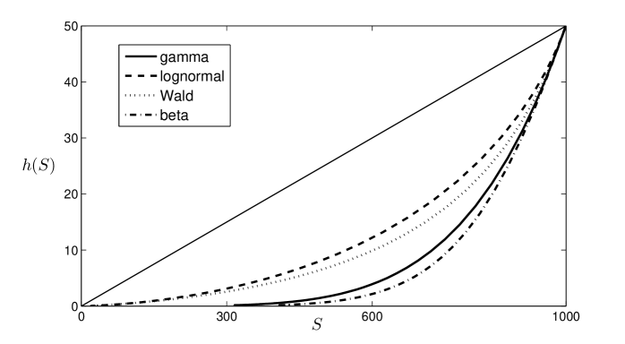
Figure 1: The functions $h(S)$ given by (16) for four different probability distributions with the same means and variances. The diagonal shows the same function for the homogeneous model $h(S)=\beta S$

The theory we briefly presented in Section 3 is equally valid both for continuous and discrete distribution. For instance, if the initial distribution is the Poisson distribution with parameter $\theta$, then we obtain

$$h(S)=S\left[\theta+\ln\left({\frac{S}{{\it S_{0}}}}\right)\right].$$ (21)

Note that in the case of the Poisson distribution there is non-zero probability that a randomly chosen individual has zero transmission coefficient, i.e., the Poisson distribution implies that some individuals are immune.

4.2 Derivation of the power transmission function

In standard epidemiological models the incidence rate (the number of new cases in a time unit) was frequently used as a bilinear function of infective and susceptible populations: $\propto SI$. In addition to this it is usually argued that there are a variety of reasons that the standard bilinear form may require modification, including the assumption of heterogeneous mixing [28, 36]. We refer to a review paper on the subject [32] for a general account of different models for incidence rates, while noting that one of the most widely used models has the form

$$\beta S^{p}I^{q},\quad p,\,q>0,$$ (22)

and is of direct interest to our study. The incidence rate in the form (22) was first used in [37], with the restriction that $p,\,q<1$, but generally it is only required that $p,q>0$, see also [29, 15, 27]. It is interesting to note in the context of our exposition that the exponents $p,\,q$ in (22) were dubbed as “heterogeneity parameters,” but the models itself is considered phenomenological and lacking mechanistical derivation [32].

A special case of (22) is $q=1$, which was considered in [38, 13]; the values for parameter $p$ were considered $p>1$. Comparison of the model (22) with the ODE (15) when the initial distribution of the susceptible subpopulation is a gamma-distribution (see (19)) let us state the following corollary.

Corollary 1.

The power relationship (22) of the incidence rate in an SIR model for the case $q=1,p>1$ can be obtained as a consequence of the heterogenous model (1)-(3) when the initial distribution of the susceptible subpopulation is a gamma-distribution.

Let us assume that not only the susceptibles are heterogeneous for some trait that influences the disease evolution, but also the infectives are heterogeneous, and consider the simplest possible SI model. Let $s(t,\omega_{1})$ and $i(t,\omega_{2})$ be the densities of the susceptibles and infectives respectively, here we assume that the traits of the two classes are independent, i.e., $\beta(\omega_{1},\omega_{2})=\beta_{1}(\omega_{1})\beta_{2}(\omega_{2})$. The number of susceptibles with the trait value $\omega_{1}$ infected by individuals with trait value $\omega_{2}$ is given by $\beta_{1}(\omega_{1})s(t,\omega_{1})\beta_{2}(\omega_{2})i(t,\omega_{2})$, and the total change in the infective class with trait value $\omega_{2}$ is $\beta_{2}(\omega_{2})i(t,\omega_{2})\int_{\Omega_{1}}\beta_{1}(\omega_{1})s(t,\omega_{1})\,d\omega_{1}$; an analogous expression applies to the change in the susceptible population. Combining the assumptions we obtain the following model:

$$\begin{split}\frac{\partial}{\partial t}s(t,\omega_{1})&=-\beta_{1}(\omega_{1})s(t,\omega_{1})\int_{\Omega_{2}}\beta_{2}(\omega_{2})i(t,\omega_{2})\,d\omega_{2}=-\beta_{1}(\omega_{1})s(t,\omega_{1})\bar{\beta}_{2}(t)I(t)\\ \frac{\partial}{\partial t}i(t,\omega_{2})&=\beta_{2}(\omega_{2})i(t,\omega_{2})\int_{\Omega_{1}}\beta_{1}(\omega_{1})s(t,\omega_{1})\,d\omega_{1}=\beta_{2}(\omega_{2})i(t,\omega_{2})\bar{\beta}_{1}(t)S(t).\end{split}$$ (23)

Model (23) is supplemented with initial conditions $s(0,\omega_{1})=S_{0}p_{s}(0,\omega_{1}),\,i(0,\omega_{2})=I_{0}p_{i}(0,\omega_{2})$. In (23) it is assumed that if an individual having trait value $\omega_{1}$ was infected by an individual with trait value $\omega_{2}$ he or she becomes an infective with trait value $\omega_{2}$ (see Section 2.2). The global dynamics of (23) is simple and is similar to the simplest homogeneous SI model.

According to Theorem 1 the system (23) can be reduced to a four-dimensional system of ODEs. Reasoning exactly as in the proof of Proposition 1 we obtain

Proposition 2.

The model (23) is equivalent to the model

$$\begin{split}\frac{d}{dt}S(t)&=-h_{1}(S)h_{2}(I),\\ \frac{d}{dt}I(t)&=h_{1}(S)h_{2}(I),\end{split}$$

where $h_{i}(x)$ is given by (16).

Combining Proposition 2 with (19) we get

Corollary 2.

The power relationship (22) of the incidence rate in an SI model for the case $q>1,p>1$ can be obtained as a consequence of the heterogenous model (23) when the initial distributions of the populations of susceptibles and infectives are gamma-distributions.

Consequently, it turns out that the power relationship (22), at least for the case $p,\,q\geqslant 1$, can be explained on the mechanistic basis by the inherent heterogeneities of the population. Its exact form is the consequence of the initial gamma-distributions, but we note that any of the transmission functions given in the previous subsection can be well approximated by (19) (see also Fig. 1).

5 The influence of population heterogeneity on the disease course

Here we mainly restrict our attention to the model (1)-(3) and study its global behavior. First we state almost obvious proposition:

Proposition 3.

Let $S_{1}(t)=\int_{\Omega}s_{1}(t,\omega)\,d\omega$ be the solution of (1)-(3) with the initial condition $s_{1}(0,\omega)=S_{0}p_{1}(0,\omega)$, and $S_{2}(t)=\int_{\Omega}s_{2}(t,\omega)\,d\omega$ be the solution of (1)-(3) with the initial condition $s_{2}(0,\omega)=S_{0}p_{2}(0,\omega)$, such that $\bar{\beta}_{1}(0)=\bar{\beta}_{1}(0)$ and $\sigma^{2}_{1}(0)>\sigma^{2}_{1}(0)$, where $\bar{\beta}_{i}(0)=\int_{\Omega}\beta(\omega)p_{i}(0,\omega)\,d\omega$ and $\sigma^{2}_{i}(0)=\int_{\Omega}(\beta(\omega)-\bar{\beta}_{i}(0))^{2}p_{i}(0,\omega)\,d\omega$, $i=1,2$. Then there exists $\varepsilon>0$ such that $S_{1}(t)>S_{2}(t)$ for all $t\in(0,\,\varepsilon)$.

The gist of this proposition is very simple: the more heterogeneous the susceptible hosts the less severe the disease progression under the model (1)-(3).

Proof.

Differentiating the first equation in (14) and using (12) we get

$$S^{\prime\prime}(t)=I^{2}S(\sigma^{2}(t)+\bar{\beta}(t))-\bar{\beta}(t)I^{\prime}S,$$

or, at the initial time moment, $S_{1}^{\prime\prime}(0)>S_{2}^{\prime\prime}(0)$. Since $S(t)$ is continuous the proposition follows. ∎

We remark that this proposition also holds for more general model (14). Moreover, we can replace equation (1) with equation

$$\frac{\partial}{\partial t}s(t,\omega)=-\beta(\omega)s(t,\omega)I(t)+s(t,\omega)[\ldots]$$

where dots denote terms describing demography, migration or the lost of immunity by removed individuals, the only condition is that these terms cannot depend on $\beta(\omega)$. Even in this case Proposition 3 still holds. For the model (5)-(6) the opposite proposition is true: the more heterogeneous the infective class in infectivity, the more severe the disease progression, which follows from the fact that $\bar{\beta}^{\prime}(t)>0$ in this case, and, consequently, $S_{1}^{\prime\prime}(0)<S_{2}^{\prime\prime}(0)$.

It is interesting to note that in the case of proportional mixing (frequency-dependent transmission) knowledge of only the initial variances of the parameter distributions does not allow inference on the short ran behavior [39].

One of the main characteristic of SIR models is the final size of the disease, which is often expressed in the number (or proportion) of susceptibles that never get infected. For the Kermack-McKendrick model

$$dS/dt=-\beta SI,\quad dI/dt=\beta SI-\gamma I,\quad dR/dt=\gamma I,$$

it is well known that the desired number, which we denote as $S(\infty)$, is given by the root of the equation

$$S(\infty)=S_{0}\exp\left\{-\frac{\beta}{\gamma}(N-S(\infty))\right\}$$ (24)

on the interval $(0,S_{0})$. Here $N$ is the constant size of the population. It is easy to show that this root always exists.

Recall that $M(0,\lambda)$ is the mgf of the initial parameter distribution. For the model (1)-(3) the following theorem holds.

Theorem 2.

The size of the susceptible subpopulation that escapes infection within the framework of the model (1)-(3) is given by the solution of the equation

$$S(\infty)=S_{0}M\left(0,(S(\infty)-N)\gamma^{-1}\right)$$ (25)

satisfying condition $0<S(\infty)<S_{0}$.

Proof.

First we note that exactly as it was done in Proposition 1, we can reduce the system (1)-(3) to the system

$$\begin{split}dS(t)/dt&=-h(S(t))I(t),\\ dI(t)/dt&=h(S(t))I(t)-\gamma I(t),\\ dR(t)/dt&=\gamma I(t).\end{split}$$ (26)

Using (16) and dividing the first equation in (26) by the third one we obtain

$$\left.\frac{dM^{-1}(0,\xi)}{d\xi}\right|_{\xi=S/S_{0}}\frac{dS}{S_{0}}=-\gamma^{-1}dR.$$

Integrating from $0$ to $\infty$ gives

$$\int_{1}^{S(\infty)/S_{0}}dM_{0}^{-1}(\xi)=-\frac{R(\infty)}{\gamma}\,.$$

Using the identities $R(\infty)=N-S(\infty)$ (since $I(\infty)=0$) and $M^{-1}(0,1)=0$ we obtain

$$M_{0}^{-1}(S(\infty)/S_{0})=-\frac{N-S(\infty)}{\gamma}\,,$$

from which (25) follows. Due to the fact that $M(0,\lambda)$ is an increasing function, the solution of (25) satisfying $0<S(\infty)<S_{0}$ is unique. ∎

Remark. If we consider nondistributed parameter (formally, we can let $\beta(\omega)=\beta=\mbox{const}$, or, equivalently, $s(0,\omega)=S_{0}\delta(\omega-\bar{\omega}),\,\beta(\bar{\omega})=\mbox{const}$, where $\delta(\omega)$ is the delta-function), we obtain (24) from (25).

Arguing in the same spirit as it is done in [5] (e.g., p. 183), the problem of the epidemic invasion can be considered. Assuming that initially all the population is susceptible (formally, for our model, $S(-\infty)=N,\,q(-\infty)=0$), from (25) the equation for the fraction of susceptible population that does not get infected follows:

$$z=M(0,-N(1-z)/\gamma).$$ (27)

Here $z=S(\infty)/N$. Equation (27) always has the root $z=1$. If the basic reproductive number [6], defined here as

$$R_{0}=\frac{\bar{\beta}(0)N}{\gamma},$$ (28)

satisfies the condition $R_{0}>1$, then there is another root of (27) in the interval $0<z<1$. This root gives the sought fraction. The proof of the existence of this root under the threshold condition $R_{0}>1$ is straightforward and can be conducted similar to the homogeneous case (e.g., [5]). This result can be illustrated by the case when the initial distribution is exponential with parameter $\nu$: the equation for $z$ is quadratic: $R_{0}z^{2}-(1+R_{0})z+1=0$, where $R_{0}=N/(\gamma\nu)$. This equation has the roots $1$ and $1/R_{0}$. If $R_{0}>1$ then the fraction of susceptible population that escapes the disease is $1/R_{0}$.

Comparing the results obtained for the heterogeneous SIR model (1)-(3) with the well known results for the simple homogeneous SIR model, we can conclude that the questions of the disease invasion can be studied in the framework of the homogeneous model because population heterogeneity does not impact the basic reproductive number (28) (this holds, obviously, if we identify the mean value of $\beta(\omega)$ over the population of susceptibles at the initial time moment with the usual constant $\beta$ in the homogeneous model). From the other hand, the heterogeneity of the population has direct impact on the final size of the disease since equation (27) depends on the initial distribution in contrast to the homogeneous analogue $z=\exp\{-R_{0}(1-z)\}$ (surprisingly, the last formula is valid under variety of different conditions [30]).

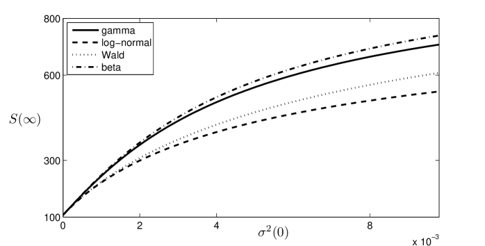
Figure 2: The size of the susceptible population that never gets infected, $S(\infty)$ versus the initial variance of the parameter distribution $\sigma^{2}(0)$ for four different initial distributions, $\bar{\beta}(0)$ is the same in all cases. The parameters are $S(0)=999,\,I(0)=1,\,\gamma=20,\,\bar{\beta}(0)=0.05$

In Fig. 2 the final size of the susceptible population versus the initial variance of the parameter distribution is shown for four different initial distributions that have the same means at $t=0$. From Fig. 2 it can be seen that the more heterogeneous the population of susceptibles, the less severe the disease not only in the short run (Proposition 3) but also globally (see [31] for the same result for frequency-dependent transmission). At the same time, it is worth emphasizing that the conditions $\bar{\beta}_{1}(0)=\bar{\beta}_{2}(0),\,\sigma^{2}_{1}(0)>\sigma^{2}_{2}(0)$ for two different initial distributions do not imply that $z_{1}>z_{2}$, where $z_{i}$ are the solutions of (27). A counterexample can be easily found (e.g., taking gamma-distribution with parameters $k=2,\,\nu=4$ and uniform distribution on the interval $[0,1]$, $N/\gamma=20$, we find that $z_{1}=0.093<z_{2}=0.112$ whereas $\sigma_{1}(0)=1/8>\sigma_{2}(0)=1/12$).

If we compare two distributions of the same family then sometimes it is possible to prove rigorously that, on the assumption of equal initial means and different second moments, more heterogeneous population (i.e., the one that has larger initial variance) experiences less severe disease. This is true, e.g., for two gamma-distributions:

Proposition 4.

Assume that we have model (1)-(3) with two initial gamma-distributions with parameters $k_{1},\nu_{1}$ and $k_{2},\nu_{2}$ such that $\bar{\beta}_{1}(0)=\bar{\beta}_{2}(0)$ and $\sigma_{1}^{2}(0)>\sigma^{2}_{2}(0)$. Assume that $R_{0}>1$. Then solutions of (27) that belong to $(0,1)$ are always satisfy $z_{1}>z_{2}$.

Proof.

We need to prove that

$$\frac{(k_{2}+R_{0}(1-z))^{k_{2}}}{(k_{1}+R_{0}(1-z))^{k_{1}}}\frac{k_{1}^{k_{1}}}{k_{2}^{k_{2}}}>1$$

for any $z\in(0,1)$. This follows from the fact that $f(r)=(k_{2}+r)^{k_{2}}/(k_{1}+r)^{k_{1}}$ is monotonically increasing function for $r>0$, i.e., $f^{\prime}(r)>0$. ∎

Remark. The last proposition can be extended to other initial distributions, e.g., it holds for Wald distribution, for a uniform distribution and some others. However, for any distribution that is not determined by its first two moments (i.e., that depends on more than two parameters) an analogous proposition is no longer true.

6 Discussion and Conclusions

Here we have presented several results concerning the course of a disease in a closed heterogeneous population, where heterogeneity is mediated by invariable traits whose distributions are determined by population structure at every time moment. One of the purposes of the present text is to introduce in the area of epidemiological modeling the general technics of the theory of heterogeneous populations [21, 23] which allows reduction of the initial infinite-dimensional dynamical system to an ODE system of a low dimension.

A usual strategy in the literature when analyzing systems similar to (1)-(3) is to consider an infinite-dimensional system of ODEs where the variables can be moments or cumulants of the corresponding distributions (e.g., [11, 33, 39]) and then analyze this system, or consider one of many possible moment-closure strategies to extract valuable information. Having the general theory outlined in Section 3 and the known results from the literature, we can critically discuss the latter and be prepared to possible pitfalls.

For example, in [11] the equation for the final epidemic size was obtained by using two different strategies: first, an initial gamma-distribution was assumed and analytical treatment was applied, and second, using the procedure suggested in [8], an approximation method was used in which the infinite-dimensional system of ODEs was replaced with two equations under the assumption that the coefficient of variation is constant. It is not surprising that Dwyer et al. obtained identical results because the gamma-distribution, according to the theory of heterogeneous populations, is the only continuous distribution which does not change its shape during the system evolution, and keeps the coefficient of variation constant (see Appendix). Therefore, the conclusion that “…the assumption of gamma-distributed susceptibility is not strictly necessary to derive equation [for the final epidemic size]” is not valid in many situations. Another initial distribution, how it is shown by (25), can yield another equation for the final epidemic size and, consequently, can produce significant discrepancy with the moment-closure approximation suggested by Dushoff [8].

The well known fact from the theory of heterogeneous populations that to model the system dynamics for a substantial time period we need to know the exact initial distribution implies that any results obtained for an epidemic in a heterogeneous population on the ground of knowledge of only several first moments of the initial distribution have to taken with extreme care. One, two, or more first moments of the initial distribution can be insufficient or even misleading. We also note that the short run behavior can be predicted when we have information only on several first moments (Section 5).

Another initial distribution which was used in the literature is the normal distribution [33]. For the normal distribution we have that $\kappa_{i}=0,\,i\geqslant 3,$ where $\kappa_{i}$ is the $i$-th cumulant. Combining the last property with the fact that the initial normal distribution remains normal within the framework of heterogeneous models we obtain that $\kappa_{i}(t)=0,\,i\geqslant 3,$ holds for any $t$ (see Appendix). This was used in [33] to obtain an explicit solution to the equation

$$\frac{\partial}{\partial t}n(t,r)=K_{g}n(t,r)-rn(t,r).$$

Here $n(t,r)$ is the number of cells at time moment $t$, which are killed by antimicrobial agents with the kill rate $r$, and $K_{g}$ is a constant (notations are changed from the original). First we note that, using Theorem 1, we obtain explicit solution of this equation for an arbitrary initial distribution of the kill rate:

$$N(t)=N_{0}M(0,-t)\exp\{K_{g}t\},$$

where $N(t)=\int_{R}n(t,r)\,dr$. Second, the results from Sections 4 and 5 cannot be applied to the normal distribution because this distribution is defined from $-\infty$ to $\infty$ and thus the corresponding mgf does not have an inverse. Which is more important, however, the total system dynamics can be influenced by these negative kill rates even if they occur with vanishingly small probability (we note that this issue is discussed in [33]). An example of such influence can be found in [24] where infinitely large growth rates occurring with small probabilities drive the population to explosion. Therefore any approximations based on an initial normal distribution in a situation where parameter can take only nonnegative values should be taken with care.

Summarizing the main results we can assert that the theory of heterogeneous populations can be successfully applied to many different mathematical models in epidemiology. Examples are given in Section 3. In many simple cases the original model can be reduced to a model described by ODEs, which simplifies the analysis. The law of mass action for a distributed susceptibility model implies a nonlinear incidence function in a homogeneous model. Moreover, one of the well known transmission functions, power relationship, follows in exact form from the initial gamma-distribution, at least in the case when exponents exceed one (see Section 4). Therefore, a mechanistic derivation has been given to the transmission power function, which was shown previously approximate real data with high accuracy. The short term behavior of the models considered can be approximately described knowing only two first moments of the initial distribution, whereas the long-term behavior depends on the exact initial distribution and can vary significantly (Section 5) even for the distributions whose several first moments are identical (Fig. 2).

It is a tempting challenge to include various demography processes to the analyzed models. The main obstacle is the need to specify the function $\phi(\omega,\omega^{\prime})$ similar to the one used in $\eqref{s1:5}$. The delta-function yields the models that can be analyzed using the general approach from Section 3 but it is usually difficult to interpret the underlying assumptions. These problems are the subject of ongoing research.

Appendix A Appendix

In Appendix we collect the definitions of the distributions used throughout the main text. The definitions are taken from [19] and [20]. In addition to that we list some facts concerning evolution of these distributions if they are used as the initial distributions for the models studies in the text. Everywhere below it is assumed that ${\beta}(\omega)=\omega$. Inasmuch as we are interested in characteristics of distributions depending on time, the following formula is very useful (see [23]):

$$M(t,\lambda)=\frac{M(0,\lambda+q(t))}{M(0,q(t))},$$ (29)

where $q(t)$ in the solution of the corresponding auxiliary differential equation (see Theorem 1), $M(t,\lambda)$ is the mgf of the parameter distribution at time $t$. Equation (29) shows that the mgf at any time instant can be expressed using the initial mgf.

Gamma-distribution

The pdf of gamma-distribution with parameters $k$ and $\nu$ is given by

$$p(0,\omega)=\frac{\nu^{k}}{\Gamma(k)}\omega^{k-1}e^{-\nu\omega},\quad\omega\geqslant 0,\,k>0,\,\nu>0.$$ (30)

The mgf of gamma-distribution is $M(0,\lambda)=(1-\lambda/\nu)^{-k}$.

It follows from (29) that for $t>0$ the distribution does not change its form, i.e., it is gamma-distribution with parameters $k$ and $s-q(t)$. The mean and variance of the distribution are given by

$$\bar{\beta}(t)=\frac{k}{s-q(t)}\,,\quad\sigma^{2}(t)=\frac{k}{(s-q(t))^{2}}\,.$$

Note that at any time moment the coefficient of variation is constant: $cv=\sigma(t)/\bar{\beta}(t)=1/\sqrt{k}$. Actually, gamma-distribution is the only continuous distribution whose coefficient of variation remains constant with time within the framework of heterogeneous models.

Wald distribution

The pdf of inverse gaussian (Wald) distribution with parameters $\mu$ and $\nu$ is

$$p(0,\omega)=\left[\frac{\nu}{2\pi\omega^{3}}\right]^{1/2}\exp\left\{-\frac{\nu}{2\mu^{2}\omega}(\omega-\mu)^{2}\right\},\quad\omega>0,\quad\mu,\,\nu>0.$$ (31)

The mgf of Wald distribution is given by

$$M(0,\lambda)=\exp\left\{\frac{\nu}{\mu}\left(1-\left[1-\frac{2\mu^{2}\lambda}{\nu}\right]^{1/2}\right)\right\}.$$

Again the distribution remains Wald distribution with parameters

$$\mu\left[1-\frac{2\mu^{2}q(t)}{v}\right]^{-\frac{1}{2}},\,\nu,$$

and temporal characteristics of the distribution are

$$\bar{\beta}(t)=\mu\left[1-\frac{2\mu^{2}q(t)}{v}\right]^{-\frac{1}{2}},\quad\sigma^{2}(t)=\frac{\bar{\beta}^{3}(t)}{\nu}\,,\quad cv^{2}=\frac{\bar{\beta}(t)}{\nu}\,.$$

Beta-distribution

Sometimes it is useful to study evolution of distribution with compact support. A good candidate in this case is the family of beta-distributions with pdf

$$p(0,\omega)=\frac{1}{B(r_{1},\,r_{2})}\frac{(\omega-a)^{r_{1}-1}(b-\omega)^{r_{2}-1}}{(b-a)^{r_{1}+r_{2}-1}}\,,\quad a\leqslant\omega\leqslant b,\,r_{1}>0,\,r_{2}>0,$$ (32)

where $B(r_{1},r_{2})$ is the beta-function.

The initial mean and variance are

$$\bar{\beta}(0)=\frac{r_{1}}{r_{1}+r_{2}},\quad\sigma^{2}(0)=\frac{r_{1}r_{2}}{(r_{1}+r_{2})^{2}(r_{1}+r_{2}+1)}\,.$$

Unfortunately in the case of beta-distribution it is impossible to write down the mgf, and, correspondingly, the temporal characteristics of the distribution. In a special case $r_{1}=r_{2}=1$ we have a uniform distribution on $[a,\,b]$. Equation (29) shows that in this case for $t>0$ the distribution is no longer uniform but turns into truncated exponential distribution.

In the text we used beta-distribution on $[0,1]$.

Log-normal distribution

The pdf of log-normal distribution defined on the nonnegative half-axis $\omega\geqslant 0$ with parameters $\mu$ and $\nu$ is

$$p(0,\omega)=\left[\omega\sqrt{2\pi}\nu\right]^{-1}\exp\left\{-\frac{1}{2}\frac{(\ln\omega-\mu)^{2}}{\nu^{2}}\right\},\quad\omega\geqslant 0,\,\mu>0,\,\nu>0.$$ (33)

The initial characteristics are

$$\beta(0)=\exp\{\mu+\nu^{2}/2\},\quad\sigma^{2}(0)=\exp\{2\mu+\nu^{2}\}(\exp\{\nu^{2}\}-1).$$

As in the case of beta-distribution we cannot present explicit formulas for the mgf and other characteristics. We note that this distribution can be used only if $q(t)<0$ for $t>0$, otherwise the integral in the mgf diverges. This is the case, e.g., for the model (1)-(3), but not the case for (6)-(7), for which the log-normal distribution cannot be used.

Normal distribution

The pdf is

$$p(0,\omega)=\left[\sqrt{2\pi}\sigma\right]^{-1}\exp\left\{-\frac{(\omega-\mu)^{2}}{2\sigma^{2}}\right\},\quad\sigma>0.$$ (34)

The mgf is $M(0,\lambda)=\exp\left\{\frac{1}{2}\lambda(2\mu+\lambda\sigma^{2})\right\}$. The temporal characteristics are

$$\bar{\beta}(t)=\mu+2q(t)\sigma^{2},\,\sigma^{2}(t)=\sigma^{2}.$$

Poisson distribution

In the same spirit discrete distributions can be managed. Consider, e.g., the Poisson distribution with parameter $\theta$, i.e,

$$p(0,\omega)=\frac{\theta^{\omega}}{\omega!}e^{\theta},\quad\theta>0,\,\omega=0,\,1,\ldots$$ (35)

then $M(0,\lambda)=\exp\left\{\theta(e^{\lambda}-1)\right\}$, and

$$\bar{\beta}(t)=\sigma(t)=\theta\exp\{q(t)\},\,cv=1.$$

Other possible initial distribution can be considered in a similar vein.

Acknowledgments. The author thanks Dr. A. Bratus’ and Dr. G. Karev for insightful discussions and helpful suggestions.

References

- [1] A. S. Ackleh. Estimation of rate distributions in generalized Kolmogorov community models. Non-Linear Analysis, 33(7):729–745, 1998.
- [2] A. S. Ackleh, D. F. Marshall, and H. E. Heatherly. Extinction in a generalized Lotka-Volterra predator-prey model. Journal of Applied Mathematics and Stochastic Analysis, 13(3):287–297, 2000.
- [3] A. S. Ackleh, D. F. Marshall, H. E. Heatherly, and B. G. Fitzpatrick. Survival of the fittest in a generalized logistic model. Mathematical Models and Methods in Applied Sciences, 9(9):1379–1391, 1999.
- [4] R. M. Anderson and R. M. C. May. Infectious Diseases of Humans: Dynamics and Control. Oxford University Press, New York, 1991.
- [5] O. Diekmann and J. A. P. Heesterbeek. Mathematical Epidemiology of Infectious Diseases: Model Building, Analysis and Interpretation. John Wiley, 2000.
- [6] O. Diekmann, J. A. P. Heesterbeek, and J. A. J. Metz. On the definition and the computation of the basic reproduction ratio in models for infectious diseases in heterogeneous populations. Journal of Mathematical Biology, 28(4):365–382, 1990.
- [7] O. Diekmann, J. A. P. Heesterbeek, and J. A. J. Metz. The legacy of Kermack and McKendrick. In D. Mollison, editor, Epidemic Models: Their Structure and Relation to Data, pages 95–115. Cambridge University Press, 1993.
- [8] J. Dushoff. Host heterogeneity and disease endemicity: A moment-based approach. Theoretical Population Biology, 56(3):325–335, 1999.
- [9] J. Dushoff and S. Levin. The effects of population heterogeneity on disease invasion. Math Biosci, 128(1-2):25–40, 1995.
- [10] G. Dwyer, J. Dushoff, J. S. Elkinton, J. P. Burand, and S. A. Levin. Host heterogeneity in susceptibility: lessons from an insect virus. In U. Diekmann, H. Metz, M. Sabelis, and K. Sigmund, editors, Virulence Managemnt: The Adaptive Dynamics of Pathogen-Host Interactions, page 74–84. Cambridge U. Press, 2002.
- [11] G. Dwyer, J. Dushoff, J. S. Elkinton, and S. A. Levin. Pathogen-driven outbreaks in forest defoliators revisited: Building models from experimental data. The American Naturalist, 156(2):105–120, 2000.
- [12] G. Dwyer, J. S. Elkinton, and J. P. Buonaccorsi. Host heterogeneity in susceptibility and disease dynamics: Tests of a mathematical model. The American Naturalist, 150(6):685–707, 1997.
- [13] V. J. Haas, A. Caliri, and M. A. A. da Silva. Temporal duration and event size distribution at the epidemic threshold. Journal of Biological Physics, 25(4):309–324, 1999.
- [14] J. A. P. Heesterbeek. The law of mass-action in epidemiology: a historical perspective. In B. E. Beisner, editor, Ecological Paradigms Lost: Routes of Theory Change, pages 81–104. Academic Press, 2005.
- [15] M. E. Hochberg. Non-linear transmission rates and the dynamics of infectious disease. J Theor Biol, 153(3):301–321, Dec 1991.
- [16] S. Hsu Schmitz. Effects of genetic heterogeneity on HIV transmission in homosexual populations. In Castillo-Chavez C. et al.(eds.), editor, Mathematical approaches for emerging and reemerging infectious diseases: Models, methods, and theory, volume 126, pages 245–260. IMA, 2002.
- [17] J. M. Hyman and J. Li. Differential susceptibility epidemic models. Journal of Mathematical Biology, 50(6):626–644, 2005.
- [18] J. A. Jacquez, C. P. Simon, and J. Koopman. Core groups and the for subgroups in heterogeneous SIS and SI models. In D. Mollison, editor, Epidemic Models: Their Structure and Relation to Data, pages 279–301. Cambrige U. Press, 1995.
- [19] N. L. Johnson, S. Kotz, and N. Balakrishnan. Continuous Univariate Distributions. Vol. 1. John Wiley, New York, 1994.
- [20] N. L. Johnson, S. Kotz, and N. Balakrishnan. Continuous Univariate Distributions. Vol 2. John Wiley, New York, 1995.
- [21] G. P. Karev. Heterogeneity effects in population dynamics. Doklady Mathematics, 62(1):141–144, 2000.
- [22] G. P. Karev. Inhomogeneous models of tree stand self-thinning. Ecological Modelling, 160(1-2):23–37, 2003.
- [23] G. P. Karev. Dynamics of heterogeneous populations and communities and evolution of distributions. Discrete and Continuous Dynamical systems, Suppl. vol.:487–496, 2005.
- [24] G. P. Karev. Dynamics of inhomogeneous populations and global demography models. Journal of Biological Systems, 13(1):83–104, 2005.
- [25] G. P. Karev, A. S. Novozhilov, and E. V. Koonin. Mathematical modeling of tumor therapy with oncolytic viruses: effects of parametric heterogeneity on cell dynamics. Biology Direct, 1(30):19, 2006.
- [26] W. O. Kermack and A. G. McKendrick. A contribution to the mathematical theory of epidemics. Proceedings of the Royal Society of London. Series A, 115(772):700–721, 1927.
- [27] R. J. Knell, M. Begon, and D. J. Thompson. Transmission dynamics of bacillus thuringiensis infecting plodia interpunctella: a test of the mass action assumption with an insect pathogen. Proc Biol Sci, 263(1366):75–81, Jan 1996.
- [28] W. M. Liu, H. W. Hethcote, and S. A. Levin. Dynamical behavior of epidemiological models with nonlinear incidence rates. J Math Biol, 25(4):359–380, 1987.
- [29] W. M. Liu, S. A. Levin, and Y. Iwasa. Influence of nonlinear incidence rates upon the behavior of SIRS epidemiological models. J Math Biol, 23(2):187–204, 1986.
- [30] J. Ma and D. J. D. Earn. Generality of the final size formula for an epidemic of a newly invading infectious disease. Bulletin of Mathematical Biology, 68(3):679–702, 2006.
- [31] R. M. May, R. M. Anderson, and M. E. Irwin. The transmission dynamics of human immunodeficiency virus (HIV). Philosophical Transactions of the Royal Society of London. Series B, Biological Sciences, 321(1207):565–607, 1988.
- [32] H. McCallum, N. Barlow, and J. Hone. How should pathogen transmission be modelled? Trends in Ecology & Evolution, 16(6):295–300, 2001.
- [33] M. Nikolaou and V. H. Tam. A new modeling approach to the effect of antimicrobial agents on heterogeneous microbial populations. Journal of Mathematical Biology, 52(2):154–182, 2006.
- [34] A. S. Novozhilov. Analysis of a generalized population predator-prey model with a parameter distributed normally over the individuals in the predator population. J. of Comput. Sys. Sci. Int., 43:378–382, 2004.
- [35] R. Ross. The Prevention of malaria. J. Murray, London, 1910.
- [36] M. Roy and M. Pascual. On representing network heterogeneities in the incidence rate of simple epidemic models. Ecological Complexity, 3(1):80–90, 2006.
- [37] N. C. Severo. Generalizations of some stochastic epidemic models. Mathematical Biosciences, 4:395–402, 1969.
- [38] P. D. Stroud, S. J. Sydoriak, J. M. Riese, J. P. Smith, S. M. Mniszewski, and P. R. Romero. Semi-empirical power-law scaling of new infection rate to model epidemic dynamics with inhomogeneous mixing. Math Biosci, 203(2):301–318, 2006.
- [39] V. M. Veliov. On the effect of population heterogeneity on dynamics of epidemic diseases. Journal of Mathematical Biology, 51(2):123–143, 2005.