Weak Measurements with Entangled Probes

Abstract

Encoding the imaginary part of a weak value onto an initially entangled probe can modify its entanglement content - provided the probe observable can distinguish between states of different entropies. Apart from fundamental interest, this result illustrates the utility of the imaginary weak value as a calculational tool in certain entanglement concentration protocols.

I Introduction

Quantum mechanics has a reputation for being rather enigmatic. This is largely due to the manner in which measurement is incorporated into the theory. Despite the ongoing controversy over the philosophical and interpretational issues surrounding quantum measurement theory, it has nonetheless proved to be a fertile ground for new exciting physics. This is particularly true for the case of weak measurements as introduced in aharonov&vaidman:1990 by Aharonov and Vaidmann. Such indirect quantum measurements follow the template established by Von Neumann vonneumman:1955 whose raison d’ tre is a circumvention of strict requirement of a classical measuring device as advocated by Bohr. Instead, the measurement device, or probe, is granted a quantum description and the ’measurement’ is regarded as the entangling of the pointer degrees of freedom of the probe with the eigen-states of the chosen observable of the system. To agree with empirical observations, the probe is then postulated to collapse into one of its pointer eigen-states by virtue of some intrinsic mechanism possibly related to its macroscopic nature. Consequently, the system collapses into a given eigen-state with its corresponding eigen-value as the measurement result.

In contrast, the unique characteristics of a weak measurement conspire to undermine the eigenvalue-measurement link axiom of quantum mechanics. Firstly, the system of interest is both pre-selected in $|i\rangle$ and post-selected in $|f\rangle$. Secondly, the coupling strength governing the interaction between system and probe is weak. As a result of these conditions, a weak measurement does not encode the eigen-values on the probe. Instead, it encodes the so-called weak value of the pre- and post-selection:

$$O_{W}=\frac{\langle f|{\hat{O}}|i\rangle}{\langle f|i\rangle}.$$ (1)

Given its form as a normalized transition amplitude, it is obvious that such weak values will not coincide with the eigen-values of the observable (provided that $|i\rangle$ or $|f\rangle$ are not eigenstates of $\hat{O}$). Perhaps more stunning, is the realization that (1) can, in general, assume complex values. The conclusion drawn from such weak measurements is that observables between pre and post-selections can possess values outside the eigen-value spectrum. In addition, one can ‘observe’ such values using a probe system coupled to the first via a weak interaction.

Originally, Aharonov and Vaidmann restricted their attention to interaction Hamiltonians of the form

$$\hat{H}_{I}=\kappa\hbar\hat{O}\otimes\hat{P},$$ (2)

where $\hat{P}$ is the conjugate pointer observable to $\hat{Q}$ with $[\hat{Q},\hat{P}]=i\hbar$. Moreover, they assumed that the probe was initially prepared in a pure Gaussian distribution of pointer eigen-states

$$|\Phi_{i}\rangle\propto\int dQ\;e^{-\frac{Q^{2}}{4\Delta^{2}Q}}|Q\rangle,$$ (3)

with the final state of the probe given as aharonov&vaidman:1990 :

$$|\Phi_{f}\rangle\propto(1-i\kappa TO_{W}\hat{P})|\Phi_{i}\rangle.$$ (4)

In the intervening years, a number of authors aharonav:2005 ; aharonov:2005 ; jozsa:2007 have characterize the back-action of weak measurements on the probe in terms of the moments of the probe’s observables. In addition, other authors johansen:2004 ; johansen&luis:2004 have illustrated that weak values can be defined even when the system and probe exist in mixed states.

In this article, we demonstrate that weak measurements can modify certain non-classical features of the probe state. In particular we show that the imaginary weak value has a r$\hat{\mbox{o}}$le in modifying the entanglement content of the probe. However, this state modification can only occur provided that the interaction Hamiltonian fulfills a certain condition. Ultimately, the probe observable must be able to distinguish between density matrices of different entropies. The exact meaning of this will become clear in section II. Apart from fundamental interest, we demonstrate, in section III, the calculational utility of the weak value formalism to aid in the understanding of certain entanglement concentration protocols fiurasek:2003 ; menzies:2006 . When viewed in this light, $\mbox{Im}(O_{W})$ provides a selection criteria to constrain the ingredients $\{|i\rangle,\hat{O},|f\rangle,\hat{K}\}$ and single out working examples of the protocol.

II Entangled Probes

To set the scene, we assume a general configuration illustrated in Figure 1.

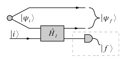
Figure 1: Mixing one of the entangled sub-systems of $|\psi_{i}\rangle$ with an ancilla system initially prepared in $|i\rangle$, before post-selecting the ancilla in the state $|f\rangle$.

The probe is initially prepared in an entangled state $|\psi_{i}\rangle\in{\cal H}^{\otimes 2}$ with Schmidt decomposition:

$$|\psi_{i}\rangle=\sum_{k=1}^{K}s_{k}|a_{k}\rangle|a_{k}\rangle.$$ (5)

The usual properties are assumed with $\{s_{k}\}_{k=1}^{K}$ obeying $\sum_{k=1}^{K}s_{k}^{2}=1$, $s_{k}\geq 0\;\forall\>k\in[1,K]$ and $\langle a_{k}|a_{j}\rangle=\delta_{jk}$. One subsystem of the probe interacts with the system initially prepared in $|i\rangle$. This mixing is provided by the interaction Hamiltonian

$$\hat{H}_{I}=\hbar\kappa\hat{K}\otimes\hat{O},$$ (6)

with, for simplicity, $\kappa=\mbox{const}$. In addition, it is assumed that all of the systems have vanishing free Hamiltonians. This can be done without loss of generality, provided we note that all results are unique up to a suitable unitary transformation. Furthermore, the observable $\hat{K}$ is required to admit the Schmidt basis as an eigen-basis with $\hat{K}|a_{k}\rangle=\lambda_{k}|a_{k}\rangle$. Consequently, the appropriate unitary evolution operator generated by (6) is

$$\hat{U}_{BC}=\exp\left(-\frac{i}{\hbar}\int_{0}^{T}dt\hat{H}_{I}\right)=e^{-i\varphi{\hat{K}}\otimes{\hat{O}}}$$ (7)

and $\varphi=\kappa T$. Following the interaction, the observable $\hat{F}$ is measured which results in the system being post-selected in a particular eigenstate $|f\rangle$ and so the final probe state is

$$|\psi_{f}\rangle\propto\langle f|\left(\hat{I}\otimes\hat{U}\right)|\psi_{i}\rangle|i\rangle.$$ (8)

The critical feature of weak measurements is the “weakness” of the coupling between probe and system, thus it is assumed that $\varphi<<1$, meaning that only linear terms are kept:

$$|\psi_{f}\rangle\approx{\cal N}\left(\langle f|i\rangle\hat{I}-i\varphi\>\langle f|\hat{O}|i\rangle(\hat{I}\otimes\hat{K})\right)|\psi_{i}\rangle.$$ (9)

Introducing the weak value of $\hat{O}$ as

$$O_{W}=\frac{\langle f|\hat{O}|i\rangle}{\langle f|i\rangle}$$ (10)

and noting that $\tilde{\cal N}={\cal N}{\langle f|i\rangle}$ allows (9) to be given as

$$|\psi_{f}\rangle=\tilde{{\cal N}}\left(\hat{I}_{AB}-i\varphi\>O_{W}(\hat{I}\otimes\hat{K})\right)|\psi_{i}\rangle,$$ (11)

with normalisation constant $\tilde{\cal N}$

$$\tilde{\cal N}\approx\frac{e^{i\phi}}{\sqrt{1+2\varphi\>\mbox{Im}(O_{W})\langle\psi_{i}|(\hat{I}\otimes\hat{K})|\psi_{i}\rangle}},$$ (12)

where $e^{i\phi}$ is an arbitrary global phase that can be set to $\phi=0$ without loss of generality. Consequently, the final entangled state is

$$|\psi_{f}\rangle=\frac{\left(\hat{I}-i\varphi\>O_{W}(\hat{I}\otimes\hat{K})\right)|\psi_{i}\rangle}{\sqrt{1+2\varphi\>\mbox{Im}(O_{W})\langle\psi_{i}|(\hat{I}\otimes\hat{K})|\psi_{i}\rangle}}.$$ (13)

From (13) it is clear that both the real and imaginary parts of the weak value contribute towards the transformation of the state. However, only the latter induces a non-unitary effect that is responsible for the modification of the entanglement content of (5). The verification of this effect requires the demonstration of a quantitative change in the entanglement content of the state. For bipartite pure states, the entanglement measure derived from the Von Neumann entropy bruss:2002 ; nielsen&chuang:2000 :

$${\cal E}(|\Psi\rangle)=\{{\cal S}\circ\mbox{Tr}_{j}\}|\Psi\rangle\langle\Psi|=-\mbox{Tr}\left(\hat{\rho}_{j}\ln\hat{\rho}_{j}\right).$$ (14)

The condition (14) holds for both subsystems $j=1,2$. The symmetric nature of the Schmidt decomposition of (5) allows us to trace out any of the two subsystems with the same result. The reduced density matrices are $\hat{\sigma}_{i}=\mbox{Tr}_{1}(\hat{\rho}_{i})$ and $\hat{\sigma}_{f}=\mbox{Tr}_{1}(\hat{\rho}_{f})$, where we denote $\hat{\rho}_{i}=|\psi_{i}\rangle\langle\psi_{i}|$ and $\hat{\rho}_{f}=|\psi_{f}\rangle\langle\psi_{f}|$. Accordingly, our starting point is the global density matrix

$$\hat{\rho}_{f}=\frac{\hat{\rho}_{i}+2\varphi\>\mbox{Im}(O_{W})\hat{K}\hat{\rho}_{i}}{1+2\varphi\>\mbox{Im}(O_{W})\mbox{Tr}(\hat{K}\hat{\sigma}_{i})},$$ (15)

which leads to the reduced density matrix

$$\hat{\sigma}_{f}=\frac{\hat{\sigma}_{i}+2\varphi\>\mbox{Im}(O_{W})\hat{K}\hat{\sigma}_{i}}{1+2\varphi\>\mbox{Im}(O_{W})\mbox{Tr}(\hat{K}\hat{\sigma}_{i})}.$$ (16)

Moreover,

$$\ln(\hat{\sigma}_{f})=\ln(\hat{\sigma}_{i}+2\varphi\>\mbox{Im}(O_{W})\hat{K}\hat{\sigma}_{i})$$

$$-\ln(1+2\varphi\>\mbox{Im}(O_{W})\mbox{Tr}(\hat{K}\hat{\sigma}_{i}))$$

$$\approx\ln(\hat{\sigma})+2\varphi\>\mbox{Im}(O_{W})\delta\hat{K},$$ (17)

where $\delta\hat{K}=\hat{K}-\mbox{Tr}(\hat{K}\hat{\sigma}_{i})$ and the second line follows from keeping only linear terms in $\varphi$. Hence

$$\hat{\sigma}_{f}\ln\hat{\sigma}_{f}=\frac{\hat{\sigma}_{i}\ln(\hat{\sigma}_{i})+2\varphi\>\mbox{Im}(O_{W})(\delta\hat{K}\sigma_{i}+\hat{K}\hat{\sigma}_{i}\ln\hat{\sigma}_{i})}{1+2\varphi\>\mbox{Im}(O_{W})\mbox{Tr}(\hat{K}\hat{\sigma}_{i})},$$ (18)

and so

$${\cal S}(\hat{\sigma}_{f})=\frac{{\cal S}(\hat{\sigma}_{i})-2\varphi\>\mbox{Tr}(\hat{K}\hat{\sigma}_{i}\ln\hat{\sigma}_{i})}{1+2\varphi\>\mbox{Im}(O_{W})\mbox{Tr}(\hat{K}\hat{\sigma}_{i})}.$$ (19)

Finally, if we note that $\hat{\omega}=\hat{\sigma}_{i}\ln\hat{\sigma}_{i}/\mbox{Tr}(\hat{\sigma}_{i}\ln\hat{\sigma}_{i})$ can be formally identified as a density matrix in its own right, then (19) becomes

$$\frac{{\cal S}(\hat{\sigma}_{f})}{{\cal S}(\hat{\sigma}_{i})}=\frac{1+2\varphi\>\mbox{Im}(O_{W})\mbox{Tr}(\hat{K}\hat{\omega})}{1+2\varphi\>\mbox{Im}(O_{W})\mbox{Tr}(\hat{K}\hat{\sigma}_{i})}.$$ (20)

The entanglement content of the probe is altered if and only if ${\cal S}_{f}\neq{\cal S}_{i}$ and so ${\cal S}_{f}/{\cal S}_{i}\neq 1$, which is true if both $\mbox{Im}(O_{W})$ and $\mbox{Tr}(\hat{K}(\hat{\sigma}_{i}-\hat{\omega}))$ cannot be zero. The requirement that $\mbox{Im}(O_{W})\neq 0$ is obvious from (13) as it accompanies a non-unitary transformation of the probe state. This follows from the properties of entanglement measures which are designed to be non-increasing under local unitary operations bruss:2002 .

On the other hand, the second simultaneous requirement that $\mbox{Tr}(\hat{K}(\hat{\omega}-\hat{\sigma}_{i}))\neq 0$ is the precise meaning to the claim that $\hat{K}$ must be able to distinguish states of different entropies given earlier. This is because the entropy of $\hat{\sigma}_{i}$ is identical to that of $\hat{\omega}$ only when the global probe state is either separable or maximally entangled. Essentially, the probe observable $\hat{K}_{B}$ must be able to witness the difference between the states $\hat{\sigma}_{i}$ and $\omega$. It is instructive to compare this requirement on $\hat{K}$ with the definition of an entanglement-witness bruss:2002 ; vedral:2006 used in the discussion of mixed state entanglement. Such a witness is a self-adjoint operator $\hat{W}$ that can distinguish between the set of separable states ${\cal S}$ and a particular entangled state $\hat{\rho}_{E}$ via $\mbox{Tr}(\hat{W}\hat{\rho})\geq 0\>\forall\hat{\rho}\in{\cal S},\;\;\mbox{Tr}(\hat{W}\hat{\rho}_{E})<0$. The essential difference between this and the r$\hat{o}$le played by $\hat{K}$ is that the latter need only distinguish between two states.

III Entanglement Concentration

It is now widely acknowledged that the counter-intuitive features of quantum states can also be interpreted as information theoretic resources. This realization has provided ample motivation for the study of quantum state engineering, with the aim of manufacturing, enhancing or repairing the desired non-classical features of a particular quantum state. Entanglement concentration protocols are designed to augment the entanglement content of a particular entangled state. From a state-engineering viewpoint, the weak measurement with an entangled probe can be interpreted as a entanglement distillation protocol. Essentially, by mixing a subsystem with an ancilla which is both pre and post-selected can augment the initial entanglement available in the global shared state. In particular, this association can be a calculational aid for Procrustean entanglement concentration protocols which modify the Schmidt coefficients whilst preserving the basis:

$$|\psi_{i}\rangle=\sum_{k=1}^{d}s_{k}|k,k\rangle\rightarrow|\psi_{f}\rangle=\sum_{k=1}^{d}t_{k}|k,k\rangle.$$ (21)

In our case, the output coefficients are a function of the weak value of the ancilla $t_{k}=f(s_{k},\varphi,O_{W})$. When viewed in this manner, we can use (22) to determine the requisite conditions on $\{|i\rangle,\hat{O},|f\rangle,\hat{K}\}$ that will collectively allow an entanglement concentration effect. Entanglement concentration of the shared state (previously known as the probe state) is given if ${\cal S}_{f}/{\cal S}_{i}>1$ and hence

$$\mbox{Im}(O_{W})\mbox{Tr}(\hat{K}(\hat{\omega}-\hat{\sigma}_{i}))>0,$$ (22)

Thus, the weak value formalism can be used in a quantum information context to single out individual examples of entanglement concentration protocols. Consequently, one can view $\mbox{Im}(O_{W})$ as a calculational aid allowing one to pick out suitable ancilla ingredients. Furthermore, in conjunction with condition on $\hat{K}$, we find the required properties of the interaction Hamiltonian to allow the desired effect.

The capacity of $\mbox{Im}(O_{W})$ as a calculational tool in entanglement concentration protocols has been previous noted by us in menzies:2007 with the example of continuous-variable states. The current work here can be regarded as a generalization to arbitrary pure bipartite entangled states.

IV Conclusion and Future Work

In conclusion, we have demonstrate the consequences of employing an initially entangled probe in weak measurements. In particular, we have shown that the entanglement content of the probe can be modified provided that the encoded weak value has a non-zero imaginary component. In addition, it is critical that the probe observable in the interaction Hamiltonian can distinguish between states of different entropies. Thus, the probe observable plays a r$\hat{o}$le similar to that of an entanglement witness with $\mbox{Tr}(\hat{K}(\hat{\omega}-\hat{\sigma}_{i}))\neq 0$. Finally, we presented evidence that the weak measurement model developed here has applications in a family of entanglement concentration protocols. Such protocols, illustrated in Figure 1, allowed for the probabilistic enhancement of an initial entangled state following a suitable interaction with an ancilla before sacrificing it to measurement. In particular, the imaginary component of a weak value can be used as selection criteria for the various ingredients $\{|i\rangle,\hat{O},|f\rangle,\hat{K}\}$ of the ancilla.

The close connection between the imaginary weak value and entanglement advocated here suggests that weak values could be regarded as a resource that can be converted into entanglement. It is then interesting to note that it has been previously established that real weak values are a source of non-classicality johansen&luis:2004 ; johansen:2004b . A natural question then arises: are imaginary weak values a source of non-classicality? If true then it could be shown that imaginary weak values are capable of modifying the non-classicality of the probe state. This would be a further generalization to the result presented here. Obtaining an answer to these questions is a future goal of our research.

References

- [1] Y. Aharonov and L. Vaidman. Phys. Rev. A. 41, 1, 11, 1990.
- [2] J. Von Neumann. Mathematical Foundations of Quantum Mechanics. Princeton Unversity Press, 1955.
- [3] Y. Aharonov and D. Rohrlich. Quantum Paradoxes: Quantum Theory for the Perplexed. Wiley-Vch, 2006.
- [4] Y. Aharonov and A. Botero. Phys. Rev. A. 72, 052111, 2005.
- [5] R. Jozsa. Phys. Rev. A. 76, 0441031, 2007.
- [6] L. M. Johansen. Phys. Rev. Lett. 93, 12, 120402, 2004.
- [7] L. M. Johansen and A. Luis. Phys. Rev. A 70, 052115, 2004.
- [8] J. Fiurek, L. Mita, and R. Filip. Phys. Rev. A 67, 022304, 2003.
- [9] D. Menzies and N. V. Korolkova. Phys. Rev. A 74, page 042315, 2006.
- [10] D. Bruss. Journ. Math. Phys. 43, page 4237, 2002.
- [11] M. Nielsen and I. Chuang. Quantum Computation and Quantum Information. Cambridge University Press, 2000.
- [12] V. Vedral. Introduction to Quantum Information Science. Oxford University Press, 2006.
- [13] D. Menzies and N. Korolkova. Phys. Rev. A 76, 062310, 2007.
- [14] L. M. Johansen. Phys. Lett. A. 329, 184, 2004.