Spiky strings, light-like Wilson loops and pp-wave anomaly

Abstract

We consider rigid rotating closed strings with spikes in AdS₅ dual to certain higher twist operators in ${\cal N}=4$ SYM theory. In the limit of large spin when the spikes reach the boundary of AdS₅, the solutions with different numbers of spikes are related by conformal transformations, implying that their energy is determined by the same function of the ‘t Hooft coupling $f(\lambda)$ that appears in the anomalous dimension of twist 2 operators or in the cusp anomaly. In the limit when the number of spikes goes to infinity, we find an equivalent description in terms of a string moving in an AdS pp-wave background. From the boundary theory point of view, the corresponding description is based on the gauge theory living in a 4d pp-wave space. Then, considering a charge moving at the speed of light, or a null Wilson line, we find that the integrated energy momentum tensor has a logarithmic UV divergence that we call the “pp-wave anomaly”. The AdS/CFT correspondence implies that, for ${\cal N}=4$ SYM, this pp-wave anomaly should have the same value as the cusp anomaly. We verify this at lowest order in SYM perturbation theory. As a side result of our string theory analysis, we find new open string solutions in the Poincare patch of the standard AdS space which end on a light-like Wilson line and also in two parallel light-like Wilson lines at the boundary.

I Introduction

The AdS/CFT correspondence provides a concrete example of the relation between gauge theories in the large-N limit and string theory malp . In particular, ${\cal N}=4$ SYM theory is seen to be dual to type IIB string theory on $AdS_{5}\times{S}^{5}$. In establishing this relation an important role is played by classical string solutions that can be mapped to “long” gauge-theory operators with large effective quantum numbers. An example is provided by strings rotating in the $S^{5}$ part of $AdS_{5}\times{S}^{5}$; it improved our understanding of the AdS/CFT and produced numerous interesting checks of the correspondence (see rev for reviews).

Another interesting case, that will concern us here, is the relation between strings rotating in ${AdS}_{5}$ and twist two operators GKP as well as its generalization to the relation between spiky strings and higher twist operators bgk ; k . In field theory at weak coupling kor ; make and also, via AdS/CFT, at strong coupling kru ; Makeenko ; krtt ; am1 ; am2 , it can be seen that the anomalouos dimension of twist two operators grw is related, for large spin, to the cusp anomaly of a light-like Wilson loop. The cusp anomaly defines a function of the ‘t Hooft coupling $f(\lambda)$,

$$E-S=f(\lambda)\ln S\ ,\ \ \ \ \ \ \ \ S\gg 1\ ,$$ (1.1)

which has been studied at small coupling using SYM perturbation theory lip and at strong coupling using $AdS_{5}\times S^{5}$ string sigma model perturbation theory ft2 ; ftt ; rt . Recently, the development of the integrability approach culminated in the proposal of an integral equation es ; bes that describes the function $f(\lambda)$ to any order in both weak bes and strong kle ; bas coupling expansion and which passed all known perturbative tests.

In the present paper we consider the higher twist operators of the general form ${\cal O}={\rm tr}\left[\left(\nabla_{+}^{\ell}\Phi\right)^{n}\right]$ which have spin $S=n\ell$ and twist $n$ and which where argued in k to be dual to certain rotating spiky string configurations in $AdS_{5}$. In the limit of large spin, keeping the number of spikes fixed, the corresponding string solutions have their spikes reaching the boundary of $AdS_{5}$ and are dual to Wilson loops with parallel light-like lines.

We study these solutions concentrating on the “arcs” between the two spikes. The shape of these arcs is determined solely by the angle $\Delta\theta=\frac{2\pi}{n}$ between the two spikes. Moreover, we show that the solutions corresponding to different values of this angle are related to one another by $SO(4,2)$ isometries of $AdS_{5}$. Since the folded rotating string of GKP is a particular $n=2$ case when the angle between the spikes is $\Delta\theta=\pi$, this implies that the anomalous dimensions of all the dual operators should be determined by the same function $f(\lambda)$.

A case of particular interest is when the angle between the adjacent spikes becomes small ($\Delta\theta\rightarrow 0$). This corresponds to the number of spikes $n$ going to infinity and one can then concentrate just on a single arc. It turns out that an appropriate way to take this limit is by a certain rescaling of the coordinates in the metric. Then the ${AdS}_{5}$ metric in global coordinates reduces to a background that can be interpreted as a pp-wave on top of ${AdS}_{5}$ in Poincare coordinates. At the same time, the boundary metric transforms from $R\times S^{3}$ to a 4d pp-wave, one which is also conformal to the Minkowski space $R^{3,1}$.

The string solution in this limit ends on two parallel light-like lines at the boundary. Computing the conserved momenta associated to such solution it follows that the function $f(\lambda)$ is determined just by a divergence near the boundary and can be found by considering a surface ending on just a single light-like line.

From the point of view of the boundary theory, i.e. gauge theory in the 4d pp-wave background, the light-like Wilson line corresponds to a point-like charge moving at the speed of light in the direction $x_{+}$ in the pp-wave metric

$$ds^{2}=2dx_{+}dx_{-}+dx_{1}^{2}+dx_{2}^{2}-(x_{1}^{2}+x_{2}^{2})dx_{+}^{2}\ .$$ (1.2)

We should then compute

$$\gamma(\lambda)=-\lim_{\varepsilon\to 0}\varepsilon\frac{\partial}{\partial\varepsilon}\ P_{+}\ ,$$ (1.3)

where $\epsilon\to 0$ is a UV cutoff and $P_{+}$ is the expectation value of the null component of the momentum operator in the presence of the Wilson line

$$P_{+}=\frac{1}{N}\int dx_{-}d^{2}x\ \sqrt{-g}\ \langle T^{+}_{+}\ {\rm tr}\ {\cal P}\big{[}e^{-ig_{{}_{\text{YM}}}\int A^{a}_{+}t^{a}dx^{+}}\big{]}\rangle|_{{}_{\text{pp-wave}}}\ .$$ (1.4)

Here $T^{\mu}_{\nu}$ is the gauge theory energy-momentum tensor. The function $\gamma(\lambda)$ which controls the divergence of the energy-momentum near the charge may be called a “pp-wave anomaly”. The analysis on the string-theory side suggests that it should be related to the twist 2 anomalous dimension, or the cusp anomaly, by

$$\gamma(\lambda)=\frac{1}{4}f(\lambda)\ .$$ (1.5)

This leads to a novel interpretation of the cusp anomaly in the case of a conformal field theory. If the gauge theory is not conformal $\gamma(\lambda)$ is not necessarily related to the cusp anomaly, and defines a new quantity which may be interesting to study.

The paper is organized as follows. In section 2 we shall consider the infinite spin limit of the spiky string solution of k and show the equivalence of its single-arc portion to the straight rotating string by performing a conformal boost in global coordinates of $AdS_{5}$.

In section 3 we shall focus on a special case when the arc between the two spikes gets small and approaches the boundary (i.e. when the number of spikes in the original solution goes to infinity). It can be studied by first taking a certain limit of the metric of the global $AdS_{5}$ space (analogous to the Penrose limit) that produces the $AdS_{5}$ metric in Poincare coordinates with a special pp-wave propagating on top of it.

In section 4 we shall find the string solution in this pp-wave background that corresponds to the original small-arc configuration, i.e. a world surface of an open string that ends on two parallel null lines at the boundary of $AdS_{5}$. We shall compute the null components of the corresponding momentum showing that $P_{+}$ has a logarithmic UV divergence and that $P_{+}\approx\frac{\sqrt{\lambda}}{2\pi}\ln P_{-}$. We shall also consider a “half-arc” solution that ends on a single null line and which is already sufficient to compute the pp-wave anomaly coefficient at strong coupling and find that it is equal to the strong-coupling value of the cusp anomaly (1.5).

In section 5 we shall perform the corresponding computation in the boundary gauge theory and confirm the relation (1.5) also at leading order in weak-coupling expansion. Section 6 will contain some concluding remarks.

In Appendix A we will show that the $AdS_{5}$ pp-wave background found in section 3 is still locally equivalent to Poincare patch of $AdS_{5}$ and also demonstrate how to construct open string solutions in $AdS_{5}$ that end on two or one null lines at the boundary. Appendix B will give details of the solution of the Maxwell equations in 4d pp-wave background with a light-like source which is used in section 5. Appendix C will contain a discussion of a generalization of the infinite spin spiky string solution from section 2 to the case of a non-zero angular momentum in $S^{5}$.

II Infinite spin limit of the spiky string

Below we shall consider a limit of the rotating spiky string of k , namely, the large spin limit, for fixed number of spikes, in which the end-points of the spikes reach the boundary of the $AdS_{5}$. Since the spiky string is a generalization of the rotating folded string of GKP , the limit is similar to the one in ft2 ; ftt . In particular, the limiting solution is sufficient in order to reproduce the large spin limit behavior of the energy ($E-S\sim\ln S$). Also, since this limiting string touches the boundary, the corresponding world-surface has, as in krtt , an open-string, i.e. Wilson loop, interpretation.

II.1 Rotating spiky string solution

Consider the ${AdS}_{3}$ part of ${AdS}_{5}$ metric

$$ds^{2}=-\cosh^{2}\rho\ dt^{2}+d\rho^{2}+\sinh^{2}\rho\ d\theta^{2}$$ (2.1)

and a rigidly rotating string configuration described by the ansatz

$$t=\tau,\ \ \ \ \ \ \theta=\omega\tau+\sigma,\ \ \ \ \ \ \ \rho=\rho(\sigma)$$ (2.2)

The Nambu string action and conserved quantities are given by

$$I = -T\int d\tau d\sigma\ \sqrt{\rho^{\prime}{}^{2}(\cosh^{2}\rho-\omega^{2}\sinh^{2}\rho)+\sinh^{2}\rho\cosh^{2}\rho}\$$ (2.3)

$$P_{t} = E=T\int d\sigma\ \frac{\cosh^{2}\rho\left(\rho^{\prime}{}^{2}+\sinh^{2}\rho\right)}{\sqrt{\rho^{\prime}{}^{2}(\cosh^{2}\rho-\omega^{2}\sinh^{2}\rho)+\sinh^{2}\rho\cosh^{2}\rho}}$$ (2.4)

$$P_{\theta} = -S=-\omega T\int d\sigma\ \frac{\rho^{\prime}{}^{2}\sinh^{2}\rho}{\sqrt{\rho^{\prime}{}^{2}(\cosh^{2}\rho-\omega^{2}\sinh^{2}\rho)+\sinh^{2}\rho\cosh^{2}\rho}}\$$ (2.5)

where $T=\frac{\sqrt{\lambda}}{2\pi}$ is the string tension and we defined the momenta as $P_{\mu}=\int\frac{\partial{\cal L}}{\partial(\partial_{\tau}X^{\mu})}d\sigma$,   $I\equiv\int d\tau d\sigma\ {\cal L}\equiv T\int d\tau d\sigma\ L$. Here $E=P_{t}$ is the energy and $S=-P_{\theta}$ is the spin.

As follows from the above action, the first integral of the equation for $\rho(\sigma)$ is k

$$-\rho^{\prime}\frac{\partial L}{\partial\rho^{\prime}}+L=\frac{\sinh^{2}2\rho}{\sqrt{(2\rho^{\prime})^{2}(\cosh^{2}\rho-\omega^{2}\sinh^{2}\rho)+\sinh^{2}2\rho}} \equiv \sinh 2\rho_{0}\ ,$$ (2.6)

where the constant of integration $\rho_{0}$ will be the minimal value of $\rho$. The maximal value $\rho=\rho_{\rm max}$ corresponds to $\cosh^{2}\rho-\omega^{2}\sinh^{2}\rho=0$, i.e. $\coth\rho_{\rm max}=\omega$. The resulting solution describes a string with spikes. For large spin we obtain the relation

$$E-S\simeq nT\ln S\ ,$$ (2.7)

where $n$ is the number of spikes and the terms we ignore are constant or vanishing in the $S\rightarrow\infty$ limit. This energy-spin relation is determined entirely by the infinite spin limit. This is also the limit when $\omega\to 1$, i.e. it corresponds to the case when the ends of the spikes approach the boundary of $AdS_{5}$. In that limit the shape of the string simplifies as we discuss in the next subsection.

II.2 Infinite spin limit

Let us consider the solution of the previous subsection in the limit when the spikes touch the ${AdS}_{5}$ boundary. Such solution corresponds to the value $\omega=1$ and gives the dominant contribution to the energy at large spin. Interestingly, it happens to have a very simple analytic form. As follows from (2.6) for $\omega=1$

$$\frac{2d\rho}{\sinh 2\rho\ \sqrt{\sinh^{2}2\rho_{0}\ \sinh^{2}2\rho-1}}=d\sigma\ ,$$ (2.8)

so that integrating this equation we get

$$\tan(\sigma+c)=\frac{\sinh 2\rho_{0}\ \cosh 2\rho}{\sqrt{\cosh^{2}2\rho-\cosh^{2}2\rho_{0}}}\ .$$ (2.9)

We can choose $c=\frac{\pi}{2}$ so that $\rho(0)=\rho_{0}$ and $\rho(\sigma\to\pm\sigma_{0})\to\infty$. Then

$$\coth 2\rho={\cos\sigma\over\cos\sigma_{0}}\ ,$$ (2.10)

$$\cot\sigma_{0}=\sinh 2\rho_{0}\ .$$ (2.11)

Equivalently,

$$\cosh 2\rho = \frac{\cos\sigma}{\sqrt{\sin^{2}\sigma_{0}-\sin^{2}\sigma}}\ ,$$

$$\sinh 2\rho = \frac{\cos\sigma_{0}}{\sqrt{\sin^{2}\sigma_{0}-\sin^{2}\sigma}}\ .$$ (2.12)

Since $\rho\rightarrow\infty$ when $\sigma\rightarrow\pm\sigma_{0}$ we have $\Delta\theta=2\sigma_{0}=\frac{2\pi}{n}$ where $n$ is the number of spikes. In general, the spiky string is a function of two parameters, the angular momentum and the number of spikes or, equivalently, $\rho_{{}_{\rm{min}}}$, and $\rho_{{}_{\rm{max}}}$ – the radii at the valleys and the spikes. Since we took $\rho_{{}_{\rm{max}}}\rightarrow\infty$, keeping $\rho_{{}_{\rm{min}}}$ fixed, only $\rho_{{}_{\rm{min}}}$ remains as a parameter, or equivalently the number of spikes given here by $\sigma_{0}$.

Since in this limit the spikes touch the boundary, we can now take only one arc between the two spikes and ignore the rest of the string. In the open-string picture krtt , this arc corresponds to a Wilson loop surface ending on two parallel light-like lines at the boundary (the spikes move at the speed of light).

Let us rewrite the above solution in the global embedding coordinates. First, note that

$$\cos\sigma=\cos(\theta-t)=\cos\theta\cos t+\sin\theta\sin t=\cos\sigma_{0}\coth 2\rho$$ (2.13)

Now, if we use the parameterization (with $Y_{3}=Y_{4}=0$)

$$Y_{1}=\sinh\rho\ \cos\theta,\ \ Y_{2}=\sinh\rho\ \sin\theta,\ \ Y_{5}=\cosh\rho\ \cos t,\ \ Y_{6}=\cosh\rho\ \sin t\$$ (2.14)

then

$$Y_{1}Y_{5}+Y_{2}Y_{6} = \cos\sigma_{0}\sinh\rho\cosh\rho\coth 2\rho$$ (2.15)

$$= \frac{1}{2}\cos\sigma_{0}\ \left(Y_{1}^{2}+Y_{2}^{2}+Y_{5}^{2}+Y_{6}^{2}\right)$$

$$= \cos\sigma_{0}\ \big{(}Y_{5}^{2}+Y_{6}^{2}-\frac{1}{2}\big{)}\ .$$

We see that the world surface as a 2d surface in $R^{4,2}$ is determined by the following system of 4 equations

$$Y_{1}^{2}+Y_{2}^{2}+Y_{3}^{2}+Y_{4}^{2}-Y_{5}^{2}-Y_{6}^{2}=-1\ ,$$

$$Y_{1}Y_{5}+Y_{2}Y_{6}-\frac{1}{2}\cos\sigma_{0}\left(Y_{1}^{2}+Y_{2}^{2}+Y_{5}^{2}+Y_{6}^{2}\right)=0\ ,$$

$$Y_{3}=Y_{4}=0\ .$$ (2.16)

Using the $SO(4,2)$ symmetry of ${AdS}_{5}$ we can put the second quadratic equation into a simple form, thus finding

$$Z_{1}^{2}+Z_{2}^{2}+Z_{3}^{2}+Z_{4}^{2}-Z_{5}^{2}-Z_{6}^{2}=-1\ ,$$

$$Z_{1}Z_{5}-Z_{2}Z_{6}=0\ ,$$ (2.17)

$$Z_{3}=Z_{4}=0\ .$$

Here $Z_{m}$ are defined by

$$Y_{1} = Z_{1}\cosh\rho_{0}+Z_{5}\sinh\rho_{0}$$

$$Y_{5} = Z_{5}\cosh\rho_{0}+Z_{1}\sinh\rho_{0}$$

$$Y_{2} = -Z_{2}\cosh\rho_{0}+Z_{6}\sinh\rho_{0}$$

$$Y_{6} = Z_{6}\cosh\rho_{0}-Z_{2}\sinh\rho_{0}\ .$$ (2.18)

We used (2.11), i.e. that $\tanh 2\rho_{0}=\cos\sigma_{0}$.

We see therefore that all solutions that we found in this limit, parameterized by $\sigma_{0}$, are actually related to one another by the two $SO(4,2)$ boosts in the 1-5 and 2-6 hyperbolic planes. Namely, a generic arc of the spiky string connecting two spikes reaching the boundary is related by these $SO(2,4)$ boosts to the infinite spin limit ft2 ; ftt of the straight folded rotating string of GKP which in our present notation corresponds to $\sigma_{0}=\frac{\pi}{2}$ or $\rho_{0}=0$ (the center of the string is at the center of $AdS_{3}$).

As follows from (2.17), this surface can be parametrized simply by

$$Z_{1} = \sinh\sigma\ \cos\tau,\ \ \ \ \ \ \ \ Z_{2}=\sinh\sigma\ \sin\tau,$$

$$Z_{5} = \cosh\sigma\ \sin\tau,\ \ \ \ \ \ \ \ Z_{6}=\cosh\sigma\ \cos\tau.$$ (2.19)

Then we get from (2.18)

$$Y_{1} = \sinh\sigma\ \cos\tau\ \cosh\rho_{0}+\ \cosh\sigma\ \sin\tau\ \sinh\rho_{0}$$

$$Y_{2} = -\sinh\sigma\ \sin\tau\ \cosh\rho_{0}+\ \cosh\sigma\ \cos\tau\ \sinh\rho_{0}$$

$$Y_{5} = \cosh\sigma\ \sin\tau\ \cosh\rho_{0}+\ \sinh\sigma\ \cos\tau\ \sinh\rho_{0}$$

$$Y_{6} = \cosh\sigma\ \cos\tau\ \cosh\rho_{0}-\ \sinh\sigma\ \sin\tau\ \sinh\rho_{0}$$ (2.20)

so that the induced metric is $ds^{2}=-d\tau^{2}+d\sigma^{2}$. This determines the expression for our solution (i.e. $t=\tau,\ \ \theta=\tau+\sigma$ and $\rho(\sigma)$ given by (2.12)) when it is transformed to conformal gauge.

As was argued in k , the spiky string state corresponds to higher twist operators with maximal anomalous dimension. The above discussion shows that, for large spin, the anomalous dimension of all such operators is determined by the same universal scaling function $f(\lambda)$ that appears for twist two operators. This is simply because the corresponding surfaces are related by conformal boosts and thus the associated string partition functions should be the same to all loop orders (see krtt ).

III “Near-boundary string” limit

The solution (2.10) found in the $S\rightarrow\infty$ limit admits two special cases. One is when the variable $\sigma_{0}$ which determines the angular distance between the two spikes ($\Delta\theta=2\sigma_{0}$) approaches ${\pi\over 2}$, i.e ${1\over 2}\Delta\theta=\sigma_{0}\to{\pi\over 2}$. Then $\rho_{0}\to 0$ and the arc becomes the straight string ($\Delta\theta=\pi$) passing through the center of $AdS_{5}$ with its ends reaching the boundary. In this limit the solution ($\coth 2\rho={1\over{\pi\over 2}-\sigma_{0}}\cos\sigma$) looks singular, implying that some rescaling is to be made.

Another special case corresponds to $\sigma_{0}\to 0$, i.e. $\rho_{0}\to\infty$, $\Delta\theta\to 0$ when the arc between the two adjacent spikes becomes small and represents an open fast-rotating string located close to the boundary with its ends moving along null lines at the boundary. According to (2.18), this case corresponds to an infinite boost of the straight string passing through the center.

In global coordinates the limit $\rho_{0}\to 0$ corresponds to no boosts in (2.18) so that $Y_{m}=Z_{m}$ in (2.19). In the limit $\rho_{0}\to\infty$ we get from (2.18)

$$Y_{1}-Y_{5}\to 0,\ \ \ Y_{1}+Y_{5}\to e^{\rho_{0}}(Z_{1}+Z_{5})\ ,$$

$$Y_{2}-Y_{6}\to 0,\ \ \ \ Y_{2}+Y_{6}\to e^{\rho_{0}}(-Z_{2}+Z_{6})\ ,$$ (3.1)

i.e. this corresponds to an infinite boost in the two (1,5),(2,6) planes.

In that second case when $\sigma_{0}$ and thus $\sigma$ are small while $\rho$ is large we can approximate the exact solution (2.2),(2.12) as:

$$t = \tau\ ,\ \ \ \ \ \ \theta=\sigma+\tau\ ,$$

$$\frac{1}{2}e^{2\rho} \simeq \frac{1}{\sqrt{\sigma_{0}^{2}-\sigma^{2}}}\ .$$ (3.2)

In this limit the ends of the string follow two light-like lines at the boundary which are very close to each other.

Since for $\sigma_{0}\to 0$ the string is located close to the boundary we may expect that we can ignore the periodicity in $\theta$ and get the corresponding solution in the Poincare patch $ds^{2}={1\over z^{2}}(-dt^{2}+dx^{2}+dz^{2})$ by identifying

$$t\to t\ ,\ \ \ \ \ \ \theta\to x\ ,\ \ \ \ \ \ \frac{1}{2}e^{-\rho}\to z\ .$$ (3.3)

The solution (3.2) then reads as

$$t = \tau\ ,\ \ \ \ \ \ \ \ x=\sigma+\tau$$

$$z = \frac{1}{2\sqrt{2}}\left(\sigma_{0}^{2}-\sigma^{2}\right)^{\frac{1}{4}}$$ (3.4)

ending at the boundary $z=0$ on the two parallel null lines $x-t\equiv x_{-}=\pm\sigma_{0}$.

However, (3.4) is not an exact solution in the Poincare patch. Still, as we shall now show, one can take a particular (infinite-boost) limit of the global ${AdS}_{5}$ metric and obtain a new metric for which eq.(3.4) will be an exact solution.

Let us start by writing the global ${AdS}_{5}$ metric as

$$ds^{2} = -\cosh^{2}\rho\ dt^{2}+d\rho^{2}+\sinh\rho^{2}\ d\Omega_{[3]}^{2}$$ (3.5)

$$= -\cosh^{2}\rho\ dt^{2}+d\rho^{2}+\sinh\rho^{2}\ \frac{(1-\frac{x_{i}^{2}}{4})^{2}\ d\theta^{2}+dx_{i}dx_{i}}{(1+\frac{x_{i}^{2}}{4})^{2}}\ ,$$

where $x_{1},x_{2}$ and $\theta$ parameterize the 3-sphere. We can now make a change of coordinates $(\rho,t,\theta)\to(z,x_{+},x_{-})$

$$\rho=-\ln(2z)\ ,\ \ \ \ \ \ \ t=x_{+}-x_{-}\ ,\ \ \ \ \ \ \theta=x_{+}+x_{-}\ ,$$ (3.6)

and a rescaling by a parameter $\varepsilon$

$$x_{+} \rightarrow \ \mu^{-1}\ x_{+}$$

$$x_{-} \rightarrow \ 8\mu\ \varepsilon^{2}\ x_{-}$$

$$x_{i} \rightarrow \ 4\varepsilon\ x_{i}$$

$$z \rightarrow \ \varepsilon\ z$$ (3.7)

Here we also introduced a (spurious) mass scale $\mu$. In the limit when $\varepsilon\to 0$ we get $\theta\to t$ and $\rho\to\infty$ while $x_{i}\to 0$, i.e. this limit focuses on a small fast-rotating string located near the boundary and near the origin of the transverse $x_{i}$ space. The end-points of the string (which are then close to its center of mass) follow the massless geodesic $t=\tau,\ \theta=\tau\pm\sigma_{0},\ x_{i}=0,\ \rho=\infty\ (z=0)$.

Taking the limit $\varepsilon\rightarrow 0$ in (3.5),(3.7) and keeping only the leading $\varepsilon$-independent terms we get the metric which such small string “sees”:

$$ds^{2}=\frac{1}{z^{2}}\left[2dx_{+}dx_{-}-\mu^{2}\left(z^{2}+x_{i}^{2}\right)dx_{+}^{2}+dx_{i}dx_{i}+dz^{2}\right]$$ (3.8)

This metric may be interpreted as a pp-wave in the ${AdS}_{5}$ space. Note that the mass parameter $\mu$ can be set to 1 by a boost in the $x_{+},x_{-}$ plane.

According to the AdS/CFT duality, the corresponding string theory should be dual to the ${\cal N}=4$ SYM gauge theory defined on the 4d pp-wave background

$$ds^{2}=2dx_{+}dx_{-}-\mu^{2}x_{i}^{2}dx_{+}^{2}+dx_{i}dx_{i}\ .$$ (3.9)

This does not contradict the fact that (3.8) was obtained as a limit of the “empty” $AdS_{5}$ space – the metric (3.9) is conformally-flat (the 5d metric (3.8) is, in fact, locally equivalent to the $AdS_{5}$ metric cha , see Appendix A).

Starting with (3.8) we can now consider two parallel light-like lines in the $x_{+}$ direction and check (see below) that there is indeed a solution of the form of (3.4), i.e. $z=z(x_{-})$, ending on them.

IV Cusp anomaly from null Wilson line in a pp-wave: strong coupling

Suppose we consider the planar ${\cal N}=4$ SYM theory in the pp-wave metric (3.9) and compute the expectation value of the Wilson loop bounded by two infinite parallel light-like lines in the direction $x_{+}$:     $x_{-}=\pm\sigma_{0},\ x_{i}=0$,  $\sigma_{0}$-const. Then according to AdS/CFT, the strong ‘t Hooft coupling limit of the expectation value of such Wilson loop should be determined maldrey by the string action for the minimal-area surface in the pp-wave metric (3.8) ending on these two null lines.

Let us find the corresponding string solution by assuming that it has the form

$$x_{+}=\tau\ ,\ \ \ \ x_{-}=\sigma,\ \ \ \ z=z(\sigma),\ \ \ \ x_{i}=0\ ,\ \ \ \ \ -\sigma_{0}\leq\sigma\leq\sigma_{0}\ .$$ (4.1)

Then the string action corresponding to (3.8) becomes

$$I=-T\int d\tau d\sigma\ \frac{1}{z^{2}}\sqrt{1+\mu^{2}z^{2}z^{\prime}{}^{2}}$$ (4.2)

Minimizing with respect to $z(\sigma)$ we obtain (we set $\mu=1$ in what follows)

$$z^{\prime}=\frac{1}{z}\sqrt{\frac{z_{0}^{4}}{z^{4}}-1}$$ (4.3)

or

$$z=\sqrt{2}(\sigma_{0}^{2}-\sigma^{2})^{\frac{1}{4}}\ ,\ \ \ \ \ \ \ \ \ \ z_{0}\equiv z_{\rm max}=\sqrt{2\sigma_{0}}\ .$$ (4.4)

For $\sigma$ changing from $-\sigma_{0}$ to $+\sigma_{0}$ we have $z$ tracing both halves of the “arc” – from 0 to $z_{0}$ and then from $z_{0}$ to 0.

This solution agrees with eq.(3.4) after a rescaling of $\sigma$ (as follows from comparing the $x_{\pm}$ part of the solution, cf. (3.4) and (3.6)), and this is again just a limit of the solution we have found in section 2.

Let us now compute the conserved quantities

$$P_{+} = -\int^{\sigma_{0}}_{-\sigma_{0}}d\sigma\ \frac{\partial{\cal L}}{\partial(\partial_{\tau}x_{+})}=T\int^{\sigma_{0}}_{-\sigma_{0}}d\sigma\ \frac{1}{z^{2}}\sqrt{1+z^{2}z^{\prime 2}}\ ,$$ (4.5)

$$P_{-} = \int^{\sigma_{0}}_{-\sigma_{0}}d\sigma\ \frac{\partial{\cal L}}{\partial(\partial_{\tau}x_{-})}=T\int^{\sigma_{0}}_{-\sigma_{0}}d\sigma\ \frac{z^{\prime 2}}{z^{2}\sqrt{1+z^{2}z^{\prime 2}}}\ .$$ (4.6)

Using eq.(4.3) we can convert the integrals over $\sigma$ into the integrals over $z$. The latter will be divergent at $z=0$ so we will insert a cut-off, $z=\epsilon\to 0$. Thus

$$P_{+} = 2T\int_{\epsilon}^{z_{0}}\frac{dz}{z\sqrt{1-\frac{z^{4}}{z^{4}_{0}}}}=T\ln{{2}z^{2}_{0}\over\epsilon^{2}}+{\cal O}(\epsilon)\ ,$$ (4.7)

$$P_{-} = 2{T}\int_{\epsilon}^{z_{0}}{dz\over z^{3}}\sqrt{1-\frac{z^{4}}{z^{4}_{0}}}=-\frac{T}{\epsilon^{2}}+\frac{\pi T}{2z_{0}^{2}}+{\cal O}(\epsilon)\ ,$$ (4.8)

where the factor of 2 reflects the fact that $(-\sigma_{0},\sigma_{0})$ covers $(\epsilon,z_{0})$ twice. Thus solving for $\epsilon$ we get

$$P_{+}\approx T\ln|P_{-}|\ .$$ (4.9)

This can be related to the spiky string expression (2.7) if we formally identify (cf. (3.6))

$$P_{+}=P_{t}+P_{\theta}=E-S,\ \ \ \ \ \ \ \ P_{-}=-P_{t}+P_{\theta}=-E-S$$ (4.10)

Then, at leading order in $\epsilon\rightarrow 0$,

$$E-S\approx T\ln{1\over\epsilon^{2}}\ ,\ \ \ \ \ \ \ \ E+S\approx\frac{T}{\epsilon^{2}}\ ,$$ (4.11)

and since, to leading order, $E\approx S$, we get

$$E-S\approx T\ln S\ .$$ (4.12)

This agrees with (2.7) since here we are considering one arc ($n=1$) of the full $n$-spike closed string.

We conclude that, if we are interested in the strong-coupling limit of anomalous the dimension of operators with large spin, it suffices to consider this particular string solution in the ${AdS}_{5}$ pp-wave background. This is analogous to the “open-string” computation of this anomalous dimension from the null cusp surface in the Poincare patch in kru ; the two world-sheet surfaces are indeed related by an analytic continuation krtt and a global-coordinate boost (3.1).

It is useful to notice that the above expressions (4.7) and (4.8) were essentially determined by the contribution near $z\sim\epsilon$, i.e. the result (4.9) follows from the properties of the solution (4.4) near the boundary. For that reason we may repeat the above discussion for a surface ending not on two but just on one null line; the role of $z_{0}$ will then be played by an explicit IR cutoff $z\leq z_{\rm max}\equiv R$.

Indeed, let us consider a world-line of a single massless “quark” at $x_{-}=0$. The corresponding “straight-string” world surface ending on this world line $x_{+}=\tau$ is then (both in the standard $AdS_{5}$ and in the $AdS_{5}$ pp-wave background (3.8))

$$x_{+}=\tau,\ \ \ \ \ \ \ \ z=\sigma,\ \ \ \ \ \ \ \ \ \ x_{-}=x_{i}=0\ .$$ (4.13)

Computing the associated momenta as in (4.5),(4.6) or (4.7),(4.8) for the case of the pp-wave background we shall cut off the integrals over $z$ at $z=\epsilon\to 0$ and at $z=L\to\infty$:

$$P_{+}=T\int^{L}_{\epsilon}dz\frac{\sqrt{\mu^{2}z^{2}}}{z^{2}}\approx{\mu T\over 2}\ln\frac{L^{2}}{\epsilon^{2}}\ ,$$ (4.14)

$$P_{-}=T\int^{\infty}_{\epsilon}dz\frac{1}{z^{2}\sqrt{\mu^{2}z^{2}}}\approx-\frac{T}{2\mu\epsilon^{2}}\ .$$ (4.15)

Here we restored the dependence on the pp-wave scale $\mu$ to indicate that a non-zero value of $P_{+}$ is found only in the pp-wave case, i.e. if $\mu\not=0$.

These expressions are one half smaller than in (4.7) and (4.8) since here we effectively have only “half” of the previous world surface that was ending on two null lines. As a result,

$$P_{+}\approx\frac{T}{2}\ln|P_{-}|={\sqrt{\lambda}\over 4\pi}\ln|P_{-}|\ ,$$ (4.16)

or, using (4.10),

$$E-S=\frac{\sqrt{\lambda}}{4\pi}\ln S\ .$$ (4.17)

Again, this is one half smaller compared to (4.12) due to the fact that here we had only one null line instead of two.

The conclusion is that in order to compute the scaling function that multiplies $\ln S$ in the anomalous dimension it is sufficient to find the UV ($z\to 0$) divergence of the momenta corresponding to the surface in the pp-wave metric (3.8) ending on the null Wilson line, i.e. on a single line in the $x_{+}$ direction.

This “elementary” or “half-arc” solution thus reproduces 1/2 of the anomaly coefficient of the two null line surface or the the one-spike solution, and thus 1/4 of the anomaly captured by straight folded rotating string (or two-spike solution).

As we shall discuss below, one can do also a similar computation for a null Wilson line in the weakly coupled gauge theory defined in the corresponding 4d pp-wave background (3.9). In the conformal gauge theory, the single null Wilson line computation will give the same result as the cusp anomaly in the fundamental representation, which is 1/4 smaller than the twist 2 anomalous dimension, i.e. the dimension of the operator like ${\rm tr}(\Phi D^{S}_{+}\Phi)$ dual to the closed folded rotating string.

V Cusp anomaly from null Wilson line in a pp-wave: weak coupling

As we have found in the previous section, an alternative way to compute the strong-coupling limit of the twist 2 anomalous dimension (or, equivalently, the cusp anomalous dimension) is to consider an open-string world surface in the “$AdS_{5}$ plus pp-wave” background (3.8) that ends on a null line at the boundary of $AdS_{5}$.

This suggests that one should be able to find the weak-coupling limit of the twist 2 anomalous dimension by considering a similar set-up in the boundary theory – the SYM gauge theory in the pp-wave background (3.9). Namely, we should study a field produced by a single charge moving at the speed of light along the $x_{+}$ direction in the 4d pp-wave background. More explicitly, we would like to reproduce the relation (4.16) at weak coupling, i.e.

$$P_{+}=\gamma(\lambda)\ln|P_{-}|\ ,$$ (5.1)

where $\gamma$ (that we may call a “pp-wave anomaly” coefficient) in the conformal gauge theory case will turn out to be proportional to the twist 2 anomalous dimension $f(\lambda)$

$$\gamma(\lambda)={1\over 4}f(\lambda)\ .$$ (5.2)

The latter has the well-known perturbative expansion grw

$$f(\lambda)={\lambda\over 2\pi^{2}}+O(\lambda^{2})\ .$$ (5.3)

The scaling function $f(\lambda)$ is proportional to the cusp anomalous dimension, i.e. it can be found also as a singular part of the expectation value of the Wilson loop with a cusp formed by two null lines in flat (Minkowski) space kor . At the lowest order in gauge coupling and in the planar limit ($\lambda=g_{{}_{\text{YM}}}^{2}N$,   $N\to\infty$) the cusp anomaly (in the fundamental representation) is

$${\Gamma}_{\mbox{cusp}}=\frac{\lambda}{8\pi^{2}}+O(\lambda^{2})={1\over 4}f(\lambda)\ .$$ (5.4)

Our aim will be to check the validity of (5.2), i.e. to reproduce (5.3) or (5.4) in the “gauge theory in pp-wave” set-up.

The null Wilson line along $x_{+}$ is BPS (both in flat space and in the pp-wave case), so the corresponding expectation value is trivial, $\langle W\rangle=1$. Instead, we are to find the logarithmic UV anomaly in the light-cone energy $P_{+}$ in the presence of a null line or the relation (5.1) between $P_{+}$ and $P_{-}$. Let us define

$$P_{\pm} \equiv \int dx_{-}d^{2}x_{i}\sqrt{-g}\ \langle\ T^{+}_{\pm}\ W\ \rangle_{{}_{\text{pp-wave}}}\ ,$$ (5.5)

$$W = \frac{1}{N}{\rm tr}\ {\cal P}e^{-ig_{{}_{\text{YM}}}\int A^{a}_{+}t^{a}dx^{+}}\ .$$ (5.6)

Here $T^{+}_{\pm}$ are the components of the gauge theory energy-momentum tensor and the expectation value is computed in the gauge theory defined in the pp-wave background (3.9). $t^{a}$ are the $SU(N)$ generators in the fundamental representation normalized as ${\rm tr}(t^{a}t^{b})=\frac{1}{2}\delta^{ab}$ ($a,b=1,2,...,N^{2}-1$).

As we shall see, $P_{+}$ will be logarithmically UV divergent and thus we may define the “pp-wave anomaly” as

$$\gamma(\lambda)=-\frac{1}{2}\lim_{\varepsilon\to 0}\varepsilon\frac{\partial}{\partial\varepsilon}\ P_{+}\ ,$$ (5.7)

where $\varepsilon\to 0$ is a UV cutoff and the factor of two is due to the fact that $P_{-}$ is quadratically divergent in the cut-off. Then (5.1) will follow from a scaling argument described below.

At lowest order in the gauge coupling the expectation value (5.5) is given simply by the one-gluon exchange, i.e. by the gaussian path integral saturated by the classical gauge field configuration with a source provided by the null Wilson line. We can then simply replace the gauge field by an abelian one $A_{\mu}$ including the factor ${C_{F}}=\frac{N^{2}-1}{2}$ from the trace in the final expression. The corresponding abelian action is then

$${\rm S}=-\frac{1}{4}\int d^{4}x\sqrt{-g}\ F^{\mu\nu}F_{\mu\nu}-g_{{}_{\text{YM}}}\int A_{+}dx^{+}\ ,\ \ \ \ \ \ \ \ \ \ \ F_{\mu\nu}=\partial_{\mu}A_{\nu}-\partial_{\nu}A_{\mu}\ .$$ (5.8)

Notice that for the pp-wave in (3.9) we have $\sqrt{-g}=1$ so we will ignore this factor in what follows.

We are then to solve the equations of motion for (5.8) ($i=1,2$)

$$\partial_{\mu}F^{\mu+}=\ g_{{}_{\text{YM}}}\ \delta(x_{-})\ \delta^{(2)}(x_{i})\ ,\ \ \ \ \ \ \ \ \ \partial_{\mu}F^{\mu-}=\partial_{\mu}F^{\mu i}=0$$ (5.9)

and evaluate (5.5) on the solution. As shown in Appendix B, the relevant solution is ($r\equiv\sqrt{x_{i}x_{i}}$)

$$A_{-} = \frac{g_{{}_{\text{YM}}}}{4\pi^{2}x_{-}}\arctan\frac{\mu r^{2}}{2x_{-}}\ ,\ \ \ \ \ \ \ \ \ \ \ A_{i}=0\ ,$$

$$A_{+} = -\frac{g_{{}_{\text{YM}}}}{4\pi^{2}}\ln\left(\mu^{2}r^{4}+4x_{-}^{2}\right)\ ,$$ (5.10)

i.e.

$$F^{+-} = F_{-+}=-\frac{2g_{{}_{\text{YM}}}}{\pi^{2}}\frac{\mu x_{-}}{\mu^{2}r^{4}+4x_{-}^{2}}\ ,$$

$$F_{+i} = \frac{g_{{}_{\text{YM}}}}{\pi^{2}}\frac{\mu^{3}r^{2}x_{i}}{\mu^{2}r^{4}+4x_{-}^{2}}\ ,\ \ \ \ \ \ F^{-i}=F_{+i}+\mu^{2}r^{2}F_{-i}=0\ ,$$

$$F^{+i} = F_{-i}=-\frac{g_{{}_{\text{YM}}}}{\pi^{2}}\frac{\mu x_{i}}{\mu^{2}r^{4}+4x_{-}^{2}}\ .$$ (5.11)

Computing the energy-momentum tensor

$$T^{\mu}{}_{\nu}=F^{\mu\alpha}F_{\alpha\nu}-\frac{1}{4}\delta^{\mu}{}_{\nu}\,F^{\alpha\beta}F_{\beta\alpha}\ ,$$ (5.12)

we get

$$T^{+}{}_{+}=\frac{g_{{}_{\text{YM}}}^{2}}{2\pi^{4}}\frac{\mu^{2}}{\mu^{2}r^{4}+4x_{-}^{2}}\ ,\ \ \ \ \ \ \ \ \ T^{+}{}_{-}=-\frac{g_{{}_{\text{YM}}}^{2}}{\pi^{4}}\frac{\mu^{2}r^{2}}{(\mu^{2}r^{4}+4x_{-}^{2})^{2}}\ .$$ (5.13)

The relevant components of the momentum (including the non-abelian group-theory factor which in the planar limit is $\frac{C_{F}}{N}\approx{N\over 2}$, see (5.5)) are

$$P_{+}=\frac{N}{2}\int^{\infty}_{-\infty}dx_{-}d^{2}x\ T^{+}{}_{+}\ ,\ \ \ \ \ \ \ P_{-}=\frac{N}{2}\int^{\infty}_{-\infty}dx_{-}d^{2}x\ T^{+}{}_{-}\ .$$ (5.14)

$P_{+}$ will be logarithmically divergent both in the UV and in the IR, while $P_{-}$ will be quadratically UV divergent. To extract this divergence it is sufficient to introduce an UV regularization in (5.13) by

$$\mu^{2}r^{4}+4x_{-}^{2}\ \rightarrow\ \mu^{2}r^{4}+4x_{-}^{2}+\mu^{2}\varepsilon^{4}\ ,\ \ \ \ \ \ \varepsilon\to 0\ .$$ (5.15)

Then doing the integrals in (5.14) we get

$$P_{+} = \frac{\lambda}{4\pi^{4}}2\pi\int_{-\infty}^{\infty}dx_{-}\int_{0}^{\infty}dr\ r\ \frac{\mu^{2}}{\mu^{2}r^{4}+4x_{-}^{2}+\mu^{2}\varepsilon^{4}}\approx{\lambda\over 8\pi^{2}}\ \mu\ \ln{L^{2}\over\varepsilon^{2}}\ ,$$ (5.16)

$$P_{-} = -\frac{\lambda}{2\pi^{4}}2\pi\int_{-\infty}^{\infty}dx_{-}\int_{0}^{\infty}dr\ r\ \frac{\mu^{2}\ r^{2}}{(\mu^{2}r^{4}+4x_{-}^{2}+\mu^{2}\varepsilon^{4})^{2}}\approx-{\lambda\over 8\pi^{2}\mu\varepsilon^{2}}\ ,$$ (5.17)

where $L\to\infty$ is an infrared cutoff ($\mu^{2}r^{4}+4x_{-}^{2}<\mu^{2}L^{4}$).

Note that, with $\lambda$ being dimensionless, the factor of $\mu$ in $P_{+}$ is necessary in order for $P_{+}$ to have the right (mass) dimension. That means that $P_{+}$ vanishes in the flat-space limit, i.e. the pp-wave background is essential for obtaining this logarithmically divergent result.

With $P_{+}$ containing the logarithmic UV divergence we can read off the corresponding anomaly coefficient as in (5.7). Equivalently, since $|P_{-}|\sim\varepsilon^{-2}\to\infty$, we find, fixing the pp-wave scale $\mu=1$,

$$P_{+}\approx\frac{\lambda}{8\pi^{2}}\ \ln|P_{-}|\ .$$ (5.18)

This is in perfect agreement with the equations (5.1),(5.2),(5.3), namely with the 1-loop value of the twist two anomalous dimension or the cusp anomalous dimension.

That $P_{+}$ should be proportional to $\ln|P_{-}|$ can be understood on general grounds and thus the relation (5.1) should be true to all orders in the expansion in $\lambda$. This follows from the following scaling argument. The pp-wave metric (3.9) is invariant, up to an overall scale, under the following transformation

$$\tilde{x}_{+}=x_{+}\ ,\ \ \ \ \ \ \ \ \tilde{x}_{-}=\xi^{2}x_{-}\ ,\ \ \ \ \ \ \ \tilde{x}_{i}=\xi x_{i}\ ,$$ (5.19)

which is the counterpart of the scaling symmetry in flat space (there is a conformal Killing vector associated to (5.19)). Since the ${\cal N}=4$ SYM theory is conformally invariant, this symmetry should be present in the quantum gauge theory. Since $x_{+}$ and $x_{-}$ scale differently in (5.19), the corresponding components of the momentum $P_{+}$ and $P_{-}$ will have different scaling weights: zero for $P_{+}$ and -2 for $P_{-}$. This implies that $P_{+}$ should be a dimensionless function of $P_{-}L^{2}$ where $L$ is an IR cutoff. Assuming the corresponding quantum state does not break the scaling symmetry spontaneously (in particular, that the classical background does not contain extra mass parameters), this function will be the logarithm.

In more detail, the ${\cal N}=4$ SYM theory defined on any conformally flat background is invariant under both diffeormorphisms and the Weyl symmetry, and, in particular, under their combination that preserves the form of the background metric (see, e.g., cft ). Thus under this combined symmetry the Wilson line factor is invariant while the gauge field strength transforms as $\tilde{F}_{\mu\nu}(\tilde{x})=\frac{\partial x^{\alpha}}{\partial\tilde{x}^{\mu}}\frac{\partial x^{\beta}}{\partial\tilde{x}^{\nu}}F_{\alpha\beta}(x)$, i.e.

$$\tilde{F}_{+-}(\tilde{x})=\xi^{-2}F_{+-}(x)\ ,\ \ \ \ \ \tilde{F}_{+i}(\tilde{x})={\xi}^{-1}F_{+i}(x)\ ,\ \ \ \ \tilde{F}_{-i}(\tilde{x})=\xi^{-3}F_{-i}(x)\ ,$$ (5.20)

Then the relevant components of the energy momentum tensor scale as

$$\tilde{T}^{+}{}_{+}(\tilde{x})=\xi^{-4}T^{+}{}_{+}(x)\ ,\ \ \ \ \ \ \tilde{T}^{+}{}_{-}(\tilde{x})=\xi^{-6}T^{+}{}_{-}(x)\ .$$ (5.21)

Thus the expectation values of their integrals in the state defined by the light-like Wilson line (which preserves the scale invariance) in (5.5) should formally scale as (the volume element $dx_{-}d^{2}x_{i}$ scales as $\xi^{4}$)

$$\tilde{P}_{+}=\xi^{0}P_{+}\ ,\ \ \ \ \ \ \tilde{P}_{-}=\xi^{-2}P_{-}\ .$$ (5.22)

In practice, as we have seen above, for these particular observables defined in (5.5) the scale invariance is broken by the UV cutoff, and (5.22) implies that $P_{+}$ in (5.14) should be logarithmically divergent whereas $P_{-}$ should be quadratically divergent.

Indeed, notice that the classical gauge field background (5.11) describing the semiclassical state defined by the Wilson loop is indeed scale-invariant, i.e. $\tilde{F}_{\mu\nu}(x)=F_{\mu\nu}(x)$ or $F_{+-}(\tilde{x})=\xi^{-2}F_{+-}(x),\ F_{+i}(\tilde{x})=\xi^{-1}F_{+i}(x),\ F_{-i}(\tilde{x})=\xi^{-3}F_{-i}(x)$ and thus $T^{+}_{+}(\tilde{x})=\xi^{-4}T^{+}{}_{+}(x),\ T^{+}_{-}(\tilde{x})=\xi^{-6}T^{+}{}_{-}(x)$. The same will, in general, apply to the expectation values defined by path integrals over the gauge fields, e.g., to the integrands in (5.5), i.e.

$${\cal T}^{+}_{+}(\tilde{x})=\xi^{-4}\ {\cal T}^{+}{}_{+}(x),\ \ \ \ {\cal T}^{+}_{-}(\tilde{x})=\xi^{-6}\ {\cal T}^{+}{}_{-}(x),\ \ \ {\cal T}^{+}_{\pm}\equiv\langle\ T^{+}_{\pm}\ W\ \rangle_{{}_{\text{pp-wave}}}\ .$$ (5.23)

Since these relations determine the dependence of ${\cal T}^{+}_{\pm}$ on the relevant radial direction in 3-space $(x_{-},x_{1},x_{2})$, namely ${\rm r}=\sqrt{r^{4}+x_{-}^{2}}$, this implies that the integrals giving $P_{+}$ and $P_{-}$ will diverge, respectively, logaritmically and quadratically at ${\rm r}\to 0$. Therefore, these divergent parts can be related as $P_{+}\sim\ln|P_{-}|$.

The relation (5.1) following from the scaling symmetry implies also that $E-S\sim\ln S$. This shows once again that the logarithmic behavior of the anomalous dimension for large spin is a consequence of the symmetries as was recently emphasized also in am2 .

Although this 1-loop check and the scaling argument are encouraging it still remains to be seen how to extend the above computation to higher loop orders.

One may wonder if the fact that the pp-wave background (3.9) is conformally-flat (see (A.1),(A.2))

$$2dx_{+}dx_{-}-\mu^{2}x^{2}_{i}dx_{+}^{2}+dx_{i}^{2}={1\over 1+\mu^{2}{\tilde{x}}_{+}^{2}}(2d{\tilde{x}}_{+}d{\tilde{x}}_{-}+d{\tilde{x}}_{i}^{2})\ ,$$ (5.24)

and that the SYM theory is conformally invariant implies that there should be an alternative way to do the above computation by staying directly in flat space. The non-trivial relation (5.18) between the $P_{+}$ and $P_{-}$ may then come out of the anomaly due to the presence of the UV cutoff that spoils the formal equivalence between the null Wilson line in the pp-wave background and its image in flat coordinates.

VI Conclusions

In this paper we have considered the large spin limit of the spiky strings in which they end at the boundary of $AdS_{5}$ and capture the $\log S$ asymptotics of the energy.

After concluding that all solutions, corresponding to different number of spikes, contain the same information about the cusp anomaly, namely $f(\lambda)$, we studied the case of an infinite number of spikes. In that limit, the solution simplified and effectively described a string moving in a 5d “AdS with pp-wave” background. Further analysis led us to an “elementary” open string solution that ends at one light-like line at the boundary and contains all the necessary information required to determine $f(\lambda)$.

The dual field theory turns out to be defined in a corresponding 4d pp-wave space. From that point of view, the essential part of the calculation that determined $f(\lambda)$ happened to be the computation of a logarithmic UV divergence in the integral of the energy momentum tensor which gives the total momentum in the light-like direction.

This led us to define a pp-wave anomaly as the coefficient of such divergence. Using AdS/CFT we derive that, for the ${\cal N}=4$ SYM theory, the pp-wave anomaly coincides with the cusp anomaly, a fact that we checked at lowest order in SYM perturbation theory. It would certainly be interesting to extend this computation to higher orders in $\lambda$ but that is beyond the scope of this paper. It is also important to point out that, similarly to what was found in am2 , in this approach, the logarithmic growth of the anomalous dimension of twist two operators for large spin is a consequence of the symmetries of the theory.

A simple way to understand why we get the field theory in a pp-wave is that when the tip of the rotating string touches the boundary it represents a field theory probe moving at the speed of light on $S^{3}$. The region near the tip of the string, which is relevant in the large spin limit, corresponds, in the boundary, to the region near such light-like trajectory. But the metric near a light-like trajectory is described by the Penrose limit of the $R\times S^{3}$ metric which is precisely the pp-wave metric. Therefore, from this point of view, the natural setup to study large spin operators is the field theory living in a pp-wave background.

To arrive at the bulk pp-wave on ${AdS}_{5}$ background (3.8) we followed a procedure similar to that of pen ; rev , namely taking a limit in the metric, in this case of ${AdS}_{5}$. By analogy to what was done in spinch for the rotation on $S^{5}$, it might be useful to consider the same limit directly in the string action. The result should be of more general nature than our present discussion and may help in understanding better the AdS/CFT correspondence in the sector states represented by strings moving in ${AdS}_{5}$ (cf. bgk ; sak ).

Finally, let us note that using the fact that the 4d pp-wave is conformally flat (and thus (3.8) is locally equivalent to $AdS_{5}$) we are able to find new string solutions in the standard $AdS_{5}$ space in Poincare coordinates, namely, the ones that end on a single light-like line, or on two parallel light-like lines. If one considers two parallel light-like Wilson lines in flat space, there is no dual string solution that respects the translation symmetry along the light-like direction. The pp-wave can perhaps be thought of as a minimal modification to the metric that allows for such a solution. If translation invariance is not imposed, then one can find such a solution in the usual Poincare patch as we show in Appendix A. It would be interesting to analyze this type of solutions further and clarify their dual field-theory interpretation.

Appendix A: Transformation from “${AdS}_{5}$ with pp-wave”
back to ${AdS}_{5}$

As was mentioned above, the field theory in the pp-wave (3.9) should be dual to string theory in the ${AdS}_{5}$ pp-wave background (3.8). It turns out that the pp-wave (3.9) is conformally flat and, as a result, the ${AdS}_{5}$ with pp-wave background (3.8) is, locally, the same as the ${AdS}_{5}$ space written in different coordinates cha . This is not totally surprising, given that (3.8) was obtained as a limit (3.7) of the standard ${AdS}_{5}$ metric in global coordinates.

To demonstrate this equivalence let us note that if we define

$$\tilde{x}_{+}=\mu^{-1}\tan\mu x_{+}\ ,\ \ \ \ \tilde{x}_{-}=x_{-}-{1\over 2}\mu x_{i}^{2}\tan\mu x_{+}\ ,\ \ \ \ \ \tilde{x}_{i}=\frac{1}{\cos\mu x_{+}}x_{i}\ ,$$ (A.1)

then

$$2d{\tilde{x}}_{+}d{\tilde{x}}_{-}+d{\tilde{x}}_{i}^{2}=\frac{1}{\cos^{2}\mu x_{+}}\left(2dx_{+}dx_{-}-\mu^{2}x^{2}_{i}dx_{+}^{2}+dx_{i}^{2}\right)\ .$$ (A.2)

A similar transformation that maps the special “${AdS}_{5}$ with pp-wave” background (3.8) into the Poincare patch of the $AdS_{5}$ is cha

$${\tilde{x}}_{+} = \mu^{-1}\tan\mu x_{+}\ ,\ \ \ \ \ \ {\tilde{x}}_{-}=x_{-}-{1\over 2}\mu(x_{i}^{2}+z^{2})\tan\mu x_{+}$$

$${\tilde{x}}_{i} = \frac{1}{\cos\mu x_{+}}x_{i}\ ,\ \ \ \ \ \tilde{z}=\frac{1}{\cos\mu x_{+}}z\ ,$$ (A.3)

i.e.

$$\frac{1}{\tilde{z}^{2}}\left(2d{\tilde{x}}_{+}d{\tilde{x}}_{-}+d{\tilde{x}}_{i}^{2}+d\tilde{z}^{2}\right)=\frac{1}{{z}^{2}}\left[2dx_{+}dx_{-}-\mu^{2}(x_{i}^{2}+{z}^{2})dx_{+}^{2}+dx_{i}^{2}+d{z}^{2}\right]\ .$$ (A.4)

Notice that the transformation (A.1) is singular at $\mu x_{+}=(2k+1)\frac{\pi}{2}$ , $k\in\mathbb{Z}$, i.e. it maps part of the pp-wave into the full flat space. Same applies to (A.3). Therefore, these pairs of spaces are equivalent only locally.

An interesting consequence of the existence of this transformation is that we can map the world-sheet surface ending on two parallel null lines (4.1),(4.3) we found in the pp-wave background (3.8) into a similar surface in the Poincare patch of ${AdS}_{5}$. The resulting surface still ends on two parallel light-like lines at the boundary and is given by (we set $\mu=1$)

$${\tilde{x}}_{+} = \tan\tau\ ,\ \ \ \ \ \ \ \ \ \ \ \ {\tilde{x}}_{i}=0$$

$${\tilde{x}}_{-} = \sigma-(\sigma_{0}^{2}-\sigma^{2})^{{1\over 2}}\,\tan\tau$$

$$\tilde{z} = \frac{\sqrt{2}}{\cos\tau}\left(\sigma_{0}^{2}-\sigma^{2}\right)^{\frac{1}{4}}\ ,$$ (A.5)

where $-\frac{\pi}{2}<\tau<\frac{\pi}{2},\ -\sigma_{0}<\sigma<\sigma_{0}$. A plot of this solution is given in fig.1.

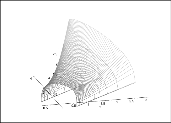
Figure 1: Surface ending on two parallel light-like Wilson lines given by $t=x\pm 1$ in ${AdS}_{5}$ space in Poincare coordinates.

Similarly, we can find a surface that is the analog of (4.13), i.e. the one that ends on a single null line in the Poincare patch of ${AdS}_{5}$ (here $\sigma>0$)

$${\tilde{x}}_{+} = \tan\tau$$

$${\tilde{x}}_{-} = -{1\over 2}\sigma^{2}\tan\tau$$

$$\tilde{z} = \frac{\sigma}{\cos\tau}\ .$$ (A.6)

This implies that

$$\tilde{z}=\sqrt{-\frac{2\tilde{x}_{-}(1+\tilde{x}_{+}^{2})}{\tilde{x}_{+}}}\ ,$$ (A.7)

where the range of $\tilde{x}_{\pm}$ is restricted by $\tilde{x}_{+}\tilde{x}_{-}<0$. This solution is depicted in fig.2. The interpretation of such solution is interesting to consider but appears unrelated to the main idea of this paper so we leave it for future work.

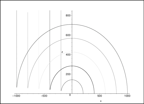
Figure 2: Surface ending on a single light-like line given by $x=t$. Here we plot the shape of the string $z(x)$ at different values of $t=200$, $400$, $600$, $800$, $1000$. The $x$-axis is the boundary where the string ends at $x=t$ (allowing to identify each curve), and its end-point we identify as a quark. In addition, there is a (rounded) spike coming out of the horizon at a point given by $x\simeq-t$ (at $x=-t$ we have $z=\infty$). The shape of the string at $t<0$ follows from the symmetry $(x,t)\rightarrow(-x,-t)$. Thus, the quark and the spike come together at $t<0$; at around $t=0$ the spike actually disappears and then reappears again on the other side moving away from the quark as shown in the figure. If we associate the spike coming out of the horizon with a gluon then this describes quark-gluon scattering but further analysis is needed in order to substantiate this interpretation.

Let us mention that a similar (euclidean) surface appeared in m (it corresponds to the case of $\omega=1$ in eq.(11) of m ):

$$z=\sqrt{\frac{2x_{-}(1-x_{+}^{2})}{x_{+}}}\ .$$ (A.8)

The surface (A.8) was shown in m to correspond to the straight infinite rotating string solution in $AdS_{5}$. This appears to be related to our observation of the equivalence of the arc between the spikes and the straight string by an $SO(2,4)$ boost made in the present paper.

Appendix B: Details of gauge theory calculation in section 5

To determine the classical field configuration which is sourced by a null Wilson like, i.e. a massless point-like charge moving along $x_{+}$ direction in the pp-wave background (3.9) we need to solve the equations following from (5.8)

$$\partial_{\mu}\left(\sqrt{-g}F^{\mu\nu}\right)=j^{\nu}\ ,$$ (B.1)

$$j^{+}=g_{{}_{\text{YM}}}\delta(x_{-})\delta^{(2)}(x_{i})\ ,\ \ \ \ \ \ \ \ j^{-}=j^{i}=0\ .$$ (B.2)

Introducing the vector potential through $F_{\mu\nu}=\partial_{\mu}A_{\nu}-\partial_{\nu}A_{\mu}$ and assuming that on symmetry grounds ($i=1,2$)

$$A_{i}=0\ ,\ \ \ \ \ \ \ A_{\pm}=A_{\pm}(r,x_{-})\ ,\ \ \ \ \ \ \ \ \ \ \ \ r^{2}\equiv x^{2}=x_{1}^{2}+x_{2}^{2}\ ,$$ (B.3)

we get

$$\partial_{-}^{2}A_{+}-\partial_{i}^{2}A_{-} = -g_{{}_{\text{YM}}}\delta(x_{-})\delta^{(2)}(x_{i})$$ (B.4)

$$-\partial_{i}^{2}A_{+}-2\mu^{2}x^{i}\partial_{i}A_{-}-\mu^{2}x^{2}\partial_{i}^{2}A_{-} = 0$$ (B.5)

$$\partial_{i}\partial_{-}A_{+}+\mu^{2}x^{2}\partial_{i}\partial_{-}A_{-} = 0\ .$$ (B.6)

The strategy that we will follow is to consider first the region $r\neq 0$ where the right hand side of (B.4) vanishes and thus we obtain a system of homogeneous equations.

From (B.6) we get ($r\equiv\sqrt{x^{2}}$)

$$\partial_{r}A_{+}=-\mu^{2}r^{2}\partial_{r}A_{-}=-\mu^{2}r^{2}\chi\ ,\ \ \ \ \ \ \ \chi\equiv\partial_{r}A_{-}\ .$$ (B.7)

Then, differentiating the first equation with respect to $r$ and eliminating $A_{+}$ using (B.7) we obtain $-\mu^{2}r^{2}\partial_{-}^{2}\chi-\partial_{r}(\partial^{2}_{r}+{1\over r}\partial_{r})A_{-}=0$, i.e.

$$-\partial_{r}^{2}\chi-\frac{1}{r}\partial_{r}\chi+\frac{1}{r^{2}}\chi-\mu^{2}r^{2}\partial_{-}^{2}\chi=0\ ,\ \ \ \ \ \ \ \chi\equiv\partial_{r}A_{-}\ .$$ (B.8)

After solving for $\chi$ we can compute $A_{\pm}$ through (B.7).

The equation for $\chi$ can be solved by first doing a Fourier transform in $x_{-}$ ($\chi(r,x_{-})\to\tilde{\chi}(r,k_{-})$)

$$-\partial_{r}^{2}\tilde{\chi}-\frac{1}{r}\partial_{r}\tilde{\chi}+(\frac{1}{r^{2}}+\mu^{2}k_{-}^{2}r^{2})\tilde{\chi}=0\ .$$ (B.9)

Integrating this equation gives

$$\tilde{\chi}(k_{-},r)=\frac{B}{r}e^{-{1\over 2}\mu|k_{-}|r^{2}}\ ,$$ (B.10)

where we pick the solution vanishing at $r\rightarrow\infty$. Here $B$ is a dimensionless constant. Fourier-transforming back in $k_{-}$ we find

$$\chi(x_{-},r)=\frac{{1\over 2}B\mu r}{\mu^{2}r^{4}+4x_{-}^{2}}\ .$$ (B.11)

This leads, using (B.7), to

$$A_{-} = \frac{B}{8x_{-}}\arctan\frac{\mu r^{2}}{2x_{-}}\ ,$$ (B.12)

$$A_{+} = -\frac{B\mu}{8}\ln(\mu^{2}r^{4}+4x_{-}^{2})\ .$$ (B.13)

The corresponding components of $F_{\mu\nu}$ are

$$F^{+-}=-F_{+-}=-\frac{B\mu x_{-}}{\mu^{2}r^{4}+4x_{-}^{2}},$$ (B.14)

$$F_{+i}=\frac{{1\over 2}B\mu^{3}r^{2}x_{i}}{\mu^{2}r^{4}+4x_{-}^{2}},\$$ (B.15)

$$F^{+i}=F_{-i}=-\frac{{1\over 2}B\mu x_{i}}{\mu^{2}r^{4}+4x_{-}^{2}}\ .$$ (B.16)

Then $\partial_{\mu}F^{\mu-}=\partial_{\mu}F^{\mu i}=0$ and

$$\partial_{\mu}F^{\mu+}=\partial_{-}F^{-+}+\partial_{i}F^{i+}=g_{{}_{\text{YM}}}\delta(x_{-})\delta^{(2)}(x_{i})\$$ (B.17)

is also satisfied away from the origin in the $(x_{1},x_{2},x_{-})$ space.

It remains to fix the constant $B$ by matching the above background onto the source. Like in the case of the usual static point-like source this can be done, for example, by regularizing the above expressions (B.16) for $F_{\mu\nu}$ near the origin $r=0,\ x_{-}=0$. Replacing there

$$\mu^{2}r^{4}+4x_{-}^{2}\ \ \to\ \ \mu^{2}r^{4}+4x_{-}^{2}+\varepsilon^{4},\ \ \ \ \ \ \ \ \ \ \varepsilon\to 0\ ,$$ (B.18)

we find

$$\partial_{-}F^{-+}+\partial_{i}F^{i+}={2B\mu\varepsilon^{4}\over(\mu^{2}r^{4}+4x_{-}^{2}+\varepsilon^{4})^{2}}\ ,\ \ \ \ \ \ \ \ \varepsilon\to 0\ .$$ (B.19)

This indeed represents the regularized delta-function in the 3-space $(x_{1},x_{2},x_{-})$ as required to match the r.h.s. of (B.17). Since

$$2\pi\int^{\infty}_{0}dr\ r\int^{\infty}_{-\infty}dx_{-}\ {2B\mu\varepsilon^{4}\over(\mu^{2}r^{4}+4x_{-}^{2}+\varepsilon^{4})^{2}}={\pi^{2}\over 2}B\ ,$$ (B.20)

we conclude that

$$B=\frac{2g_{{}_{\text{YM}}}}{\pi^{2}}\ .$$ (B.21)

Thus finally we find from (B.12),(B.16),(B.21) the expressions (5.10),(5.11) used in the main text.

Let us note that the scale $\mu$ of the pp-wave (3.9) plays the role of a regularizing parameter for the above solution. Since the one-dimensional delta-function has the representation

$$\delta(y)=\frac{1}{\pi}\lim_{\mu\to 0}\frac{\mu}{y^{2}+\mu^{2}}\ ,$$ (B.22)

we conclude that in the flat-space limit $\mu\to 0$ the above solution becomes

$$F^{+-} = -\frac{2g_{{}_{\text{YM}}}}{\pi}\ {x_{-}\over r^{4}}\ \delta({2x_{-}\over r^{2}})=-\frac{g_{{}_{\text{YM}}}}{\pi}\ {x_{-}\over r^{2}}\ \delta({x_{-}})=0,\ \ \ F_{+i}=0$$

$$F^{+i} = -\frac{g_{{}_{\text{YM}}}}{\pi}\ {x_{i}\over r^{4}}\ \delta({2x_{-}\over r^{2}})=-\frac{g_{{}_{\text{YM}}}}{2\pi}\ {x_{i}\over r^{2}}\ \delta({x_{-}})\ .$$ (B.23)

These expressions formally give $T^{+}_{+}=0$. In this sense switching on the pp-wave background provides a regularization of the problem of finding the field produced by a point-like charge moving with the speed of light.

Appendix C: Generalization of solution in section 2.2
to rotation in $S^{5}$

The conformal-gauge parametrization in (2.20) is useful for generalizing the above “one-arc” solution (2.11)–(2.12) to the case when the string has also a momentum $J$ along a circle in $S^{5}$. All we need to do is to generalize first the straight string solution (i.e. (2.19)) and then apply the two boosts as in (2.18). The point is that this generalization modifies only the conformal gauge constraints, but in the embedding coordinate parametrization in conformal gauge both the sigma model equations and the constraints are covariant under the $SO(2,4)$ transformations.

The conformal-gauge solution for the straight infinite string stretching to the boundary of $AdS_{5}$ that rotates both in $AdS_{5}$ and $S^{5}$ with spins $S$ and $J$ is given by ftt :

$$t=\kappa\tau,\ \ \ \rho=\mu\sigma,\ \ \ \ \theta=\kappa\tau,\ \ \ \ \varphi=\nu\tau\ ,$$ (C.1)

$$\kappa^{2}=\mu^{2}+\nu^{2}\ ,\ \ \ \mu={1\over\pi}\ln{S\over\sqrt{\lambda}}\gg 1\ ,\ \ \ \nu={J\over\sqrt{\lambda}}\ ,\ \ \ \ \ell\equiv{\nu\over\mu}={\rm fixed}$$ (C.2)

where we use the $AdS_{5}$ metric in (2.1) and $\varphi$ is an angle in $S^{5}$. The corresponding solution in the embedding coordinates is (cf. (2.19))

$$Z_{5}+iZ_{6}=\cosh\mu\sigma\ e^{i\kappa\tau}\ ,\ \ \ \ \ \ \ Z_{1}+iZ_{2}=\sinh\mu\sigma\ e^{i\kappa\tau}\ .$$ (C.3)

We may then use double-boost transformation (2.20) to construct the corresponding solution with non-zero $\rho_{0}$:

$$Y_{1} = \sinh\mu\sigma\cos\kappa\tau\ \cosh\rho_{0}-\cosh\mu\sigma\sin\kappa\tau\ \sinh\rho_{0}$$

$$Y_{2} = -\sinh\mu\sigma\sin\kappa\tau\ \cosh\rho_{0}+\cosh\mu\sigma\cos\kappa\tau\ \sinh\rho_{0}$$

$$Y_{5} = \cosh\mu\sigma\sin\kappa\tau\ \cosh\rho_{0}+\sinh\mu\sigma\cos\kappa\tau\ \sinh\rho_{0}$$

$$Y_{6} = \cosh\mu\sigma\cos\kappa\tau\ \cosh\rho_{0}-\sinh\mu\sigma\sin\kappa\tau\ \sinh\rho_{0}$$ (C.4)

It is straightforward now to construct explicitly the corresponding expressions for $t^{\prime},\rho^{\prime},\theta^{\prime}$ coordinates defined by

$$Y_{5}+iY_{6}=\cosh\rho^{\prime}\ e^{it^{\prime}}\ ,\ \ \ \ \ \ \ Y_{1}+iY_{2}=\sinh\rho^{\prime}\ e^{i\theta^{\prime}}\ ,$$ (C.5)

and find the energy and spin generators and a relation between them.

Note that the generalization of eqs. (2.3) and (2.6) to non-zero $S^{5}$ rotation parameter $\nu$ are

$$I=-T\int d\sigma d\tau\ \sqrt{\rho^{\prime}{}^{2}(\cosh^{2}\rho-\omega^{2}\sinh^{2}\rho-\nu^{2})+\sinh^{2}\rho\ (\cosh^{2}\rho-\nu^{2})},$$

$${\sinh^{2}\rho\ (\cosh^{2}\rho-\nu^{2})\over\sqrt{\rho^{\prime 2}\ (\cosh^{2}\rho-\omega^{2}\sinh^{2}\rho-\nu^{2})+\sinh^{2}\rho\ (\cosh^{2}\rho-\nu^{2})}}$$

$$\ \ \ \ \ \ \ \ \ \ \ =\sinh\rho_{0}\ \sqrt{\cosh^{2}\rho_{0}-\nu^{2}}\ ,$$ (C.6)

where the constant of integration $\rho_{0}$ is again the minimal value of $\rho=\rho_{\rm min}$. The maximal value of $\rho$ corresponds now to $\coth^{2}\rho_{\rm max}={\omega^{2}-\nu^{2}\over 1-\nu^{2}}$, it can become infinite, i.e. the spikes can reach the boundary, provided $\omega=1$, namely $\theta=t$. Notice that this is the case we are considering in eq.(C.1).

References

- (1)
- (2) J. M. Maldacena, “The large N limit of superconformal field theories and supergravity,” Adv. Theor. Math. Phys. 2, 231 (1998) [arXiv:hep-th/9711200]. S. S. Gubser, I. R. Klebanov and A. M. Polyakov, “Gauge theory correlators from non-critical string theory,” Phys. Lett. B 428, 105 (1998) [arXiv:hep-th/9802109]. E. Witten, “Anti-de Sitter space and holography,” Adv. Theor. Math. Phys. 2, 253 (1998) [arXiv:hep-th/9802150]. O. Aharony, S. S. Gubser, J. M. Maldacena, H. Ooguri and Y. Oz, “Large N field theories, string theory and gravity,” Phys. Rept. 323, 183 (2000) [arXiv:hep-th/9905111].
- (3) D. E. Berenstein, J. M. Maldacena and H. S. Nastase, “Strings in flat space and pp waves from N = 4 super Yang Mills,” JHEP 0204, 013 (2002) [arXiv:hep-th/0202021]. D. Sadri and M. M. Sheikh-Jabbari, “The plane-wave / super Yang-Mills duality,” Rev. Mod. Phys. 76, 853 (2004) [arXiv:hep-th/0310119]. A. A. Tseytlin, “Spinning strings and AdS/CFT duality,” arXiv:hep-th/0311139. N. Beisert, “The dilatation operator of N = 4 super Yang-Mills theory and integrability,” Phys. Rept. 405, 1 (2005) [arXiv:hep-th/0407277]. J. Plefka, “Spinning strings and integrable spin chains in the AdS/CFT correspondence,” arXiv:hep-th/0507136.
- (4) S. S. Gubser, I. R. Klebanov and A. M. Polyakov, “A semi-classical limit of the gauge/string correspondence,” Nucl. Phys. B 636, 99 (2002) [arXiv:hep-th/0204051].
- (5) A. V. Belitsky, A. S. Gorsky and G. P. Korchemsky, “Gauge / string duality for QCD conformal operators,” Nucl. Phys. B 667, 3 (2003) [arXiv:hep-th/0304028].
-
(6)
M. Kruczenski,
“Spiky strings and single trace operators in gauge theories,”
JHEP 0508, 014 (2005)
[arXiv:hep-th/0410226],
M. Kruczenski, J. Russo and A. A. Tseytlin, “Spiky strings and giant magnons on S5,” JHEP 0610, 002 (2006) [arXiv:hep-th/0607044]. - (7) A.M. Polyakov, “Gauge Fields As Rings Of Glue,” Nucl. Phys. B 164, 171 (1980). G. P. Korchemsky, “Asymptotics of the Altarelli-Parisi-Lipatov Evolution Kernels of Parton Distributions,” Mod. Phys. Lett. A 4, 1257 (1989). G. P. Korchemsky and G. Marchesini, “Structure function for large x and renormalization of Wilson loop,” Nucl. Phys. B 406, 225 (1993) [arXiv:hep-ph/9210281].
- (8) Y. Makeenko, P. Olesen and G. W. Semenoff, “Cusped SYM Wilson loop at two loops and beyond,” Nucl. Phys. B 748, 170 (2006) [arXiv:hep-th/0602100].
- (9) M. Kruczenski, “A note on twist two operators in N = 4 SYM and Wilson loops in Minkowski signature,” JHEP 0212, 024 (2002) [arXiv:hep-th/0210115].
- (10) Y. Makeenko, “Light-cone Wilson loops and the string / gauge correspondence,” JHEP 0301, 007 (2003) [arXiv:hep-th/0210256].
- (11) M. Kruczenski, R. Roiban, A. Tirziu and A. A. Tseytlin, “Strong-coupling expansion of cusp anomaly and gluon amplitudes from quantum open strings in AdS5 x S5,” Nucl. Phys. B 791, 93 (2008) [arXiv:0707.4254 [hep-th]].
- (12) L. F. Alday and J. Maldacena, “Gluon scattering amplitudes at strong coupling,” arXiv:0705.0303 [hep-th].
- (13) L. F. Alday and J. M. Maldacena, “Comments on operators with large spin,” JHEP 0711, 019 (2007) [arXiv:0708.0672 [hep-th]].
- (14) D.J. Gross and F. Wilczek, “Asymptotically free gauge theories. 2,” Phys. Rev. D 9, 980 (1974).
- (15) A. V. Kotikov, L. N. Lipatov, A. I. Onishchenko and V. N. Velizhanin, “Three-loop universal anomalous dimension of the Wilson operators in N = 4 SUSY Yang-Mills model,” Phys. Lett. B 595, 521 (2004) [Erratum-ibid. B 632, 754 (2006)] [arXiv:hep-th/0404092]. Z. Bern, M. Czakon, L. J. Dixon, D. A. Kosower and V. A. Smirnov, “The Four-Loop Planar Amplitude and Cusp Anomalous Dimension in Maximally Supersymmetric Yang-Mills Theory,” Phys. Rev. D 75, 085010 (2007) [arXiv:hep-th/0610248]. F. Cachazo, M. Spradlin and A. Volovich, “Four-Loop Cusp Anomalous Dimension From Obstructions,” Phys. Rev. D 75, 105011 (2007) [arXiv:hep-th/0612309].
- (16) S. Frolov and A. A. Tseytlin, “Semiclassical quantization of rotating superstring in AdS(5) x S(5),” JHEP 0206, 007 (2002) [arXiv:hep-th/0204226].
- (17) S. Frolov, A. Tirziu and A. A. Tseytlin, “Logarithmic corrections to higher twist scaling at strong coupling from AdS/CFT,” Nucl. Phys. B 766, 232 (2007) [arXiv:hep-th/0611269].
- (18) R. Roiban, A. Tirziu and A. A. Tseytlin, “Two-loop world-sheet corrections in superstring,” JHEP 0707, 056 (2007) [arXiv:0704.3638 [hep-th]]. R. Roiban and A. A. Tseytlin, “Strong-coupling expansion of cusp anomaly from quantum superstring,” JHEP 0711, 016 (2007) [arXiv:0709.0681 [hep-th]].
- (19) B. Eden and M. Staudacher, “Integrability and transcendentality,” J. Stat. Mech. 0611, P014 (2006) [arXiv:hep-th/0603157].
- (20) N. Beisert, B. Eden and M. Staudacher, “Transcendentality and crossing,” J. Stat. Mech. 0701, P021 (2007) [arXiv:hep-th/0610251].
- (21) M. K. Benna, S. Benvenuti, I. R. Klebanov and A. Scardicchio, “A test of the AdS/CFT correspondence using high-spin operators,” Phys. Rev. Lett. 98, 131603 (2007) [arXiv:hep-th/0611135]. L. F. Alday, G. Arutyunov, M. K. Benna, B. Eden and I. R. Klebanov, “On the strong coupling scaling dimension of high spin operators,” JHEP 0704, 082 (2007) [arXiv:hep-th/0702028].
- (22) B. Basso, G. P. Korchemsky and J. Kotanski, “Cusp anomalous dimension in maximally supersymmetric Yang-Mills theory at strong coupling,” arXiv:0708.3933 [hep-th].
- (23) M. Abbott, private communication.
- (24) J. M. Maldacena, “Wilson loops in large N field theories,” Phys. Rev. Lett. 80, 4859 (1998) [arXiv:hep-th/9803002]. S. J. Rey and J. T. Yee, “Macroscopic strings as heavy quarks in large N gauge theory and anti-de Sitter supergravity,” Eur. Phys. J. C 22, 379 (2001) [arXiv:hep-th/9803001]. N. Drukker, D. J. Gross and H. Ooguri, “Wilson loops and minimal surfaces,” Phys. Rev. D 60, 125006 (1999) [arXiv:hep-th/9904191].
- (25) M. Cvetic, H. Lu and C. N. Pope, “Spacetimes of boosted p-branes, and CFT in infinite-momentum frame,” Nucl. Phys. B 545, 309 (1999) [arXiv:hep-th/9810123].
- (26) D. Brecher, A. Chamblin and H. S. Reall, “AdS/CFT in the infinite momentum frame,” Nucl. Phys. B 607, 155 (2001) [arXiv:hep-th/0012076].
- (27) R. R. Metsaev, “Supersymmetric D3 brane and N = 4 SYM actions in plane wave backgrounds,” Nucl. Phys. B 655, 3 (2003) [arXiv:hep-th/0211178]. “Superfield formulation of N = 4 super Yang-Mills theory in plane wave background,” arXiv:hep-th/0301009.
- (28) C. S. Chu and P. M. Ho, “Time-dependent AdS/CFT Duality II: Holographic Reconstruction of Bulk Metric and Possible Resolution of Singularity,” arXiv:0710.2640 [hep-th]. “Time-dependent AdS/CFT duality and null singularity,” JHEP 0604, 013 (2006) [arXiv:hep-th/0602054]. A. Awad, S. R. Das, K. Narayan and S. P. Trivedi, “Gauge Theory Duals of Cosmological Backgrounds and their Energy Momentum Tensors,” arXiv:0711.2994 [hep-th]. S. R. Das, J. Michelson, K. Narayan and S. P. Trivedi, “Cosmologies with null singularities and their gauge theory duals,” Phys. Rev. D 75, 026002 (2007) [arXiv:hep-th/0610053]. F. L. Lin and D. Tomino, “One-loop effect of null-like cosmology’s holographic dual super-Yang-Mills,” JHEP 0703, 118 (2007) [arXiv:hep-th/0611139].
- (29) M. Kruczenski, “Wilson loops and anomalous dimensions in cascading theories,” Phys. Rev. D 69, 106002 (2004) [arXiv:hep-th/0310030].
- (30) M. Blau, J. Figueroa-O’Farrill, C. Hull and G. Papadopoulos, “Penrose limits and maximal supersymmetry,” Class. Quant. Grav. 19, L87 (2002) [arXiv:hep-th/0201081]. K. Sfetsos and A. A. Tseytlin, “Four-dimensional plane wave string solutions with coset CFT description,” Nucl. Phys. B 427, 245 (1994) [arXiv:hep-th/9404063].
- (31) E. S. Fradkin and A. A. Tseytlin, “Conformal Supergravity,” Phys. Rept. 119, 233 (1985). E. S. Fradkin and M. Y. Palchik, “Conformal quantum field theory in D-dimensions,” Dordrecht, Netherlands: Kluwer (1996) 461 p. (Mathematics and its applications. 376)
- (32) M. Kruczenski, “Spin chains and string theory,”, Phy. Rev. Lett 93, 161602 (2004), [arXiv:hep-th/0311203]. M. Kruczenski, A. V. Ryzhov and A. A. Tseytlin, “Large spin limit of AdS(5) x S5 string theory and low energy expansion of ferromagnetic spin chains,” Nucl. Phys. B 692, 3 (2004) [arXiv:hep-th/0403120]. M. Kruczenski and A. A. Tseytlin, “Semiclassical relativistic strings in S5 and long coherent operators in N = 4 SYM theory,” JHEP 0409, 038 (2004) [arXiv:hep-th/0406189]. R. Hernandez and E. Lopez, “The SU(3) spin chain sigma model and string theory,” JHEP 0404, 052 (2004) [arXiv:hep-th/0403139].
- (33) K. Sakai and Y. Satoh, “A large spin limit of strings on AdS(5) x S5 in a non-compact sector,” Phys. Lett. B 645, 293 (2007) [arXiv:hep-th/0607190].
- (34) R. Gueven, “The conformal Penrose limit and the resolution of the pp-curvature singularities,” Class. Quant. Grav. 23, 295 (2006) [arXiv:hep-th/0508160].