A Multi-wavelength Study of the Massive Star-forming Region S87

Abstract

This article presents a multi-wavelength study towards the massive star-forming region S87, based on a dataset of submillimeter/far-/mid-infrared (sub-mm/FIR/MIR) images and molecular line maps. The sub-mm continuum emission measured with JCMT/SCUBA reveals three individual clumps, namely, SMM 1, SMM 2, and SMM 3. The MIR/FIR images obtained by the Spitzer Space Telescope indicate that both SMM 1 and SMM 3 harbor point sources. The J = 1 – 0 transitions of CO, ¹³CO, C¹⁸O, and HCO⁺, measured with the 13.7 m telescope of the Purple Mountain Observatory, exhibit asymmetric line profiles. Our analysis of spectral energy distributions (SEDs) shows that all of the three sub-mm clumps are massive (110 — 210 $M_{\odot}$), with average dust temperatures in the range $\sim$ 20 —40 K. A multi-wavelength comparison convinces us that the asymmetric profiles of molecular lines should result from two clouds at slightly different velocities, and it further confirms that the star-forming activity in SMM 1 is stimulated by a cloud-cloud collision. The stellar contents and SEDs suggest that SMM 1 and SMM 3 are high-mass and intermediate-mass star-forming sites respectively. However, SMM 2 has no counterpart downwards 70 $\mu$m, which is likely to be a cold high-mass starless core. These results, as mentioned above, expose multiple phases of star formation in S87.

1 INTRODUCTION

Massive stars play an important role in the evolution of the interstellar medium (ISM) and galaxies; nevertheless their formation process is still poorly understood from the observational perspective because of their relatively short evolution periods, complex ambient circumstances and gregarious nature. Two important approaches are systematic surveys and multi-wavelength studies towards individual sources to increase our knowledge about high-mass molecular cores that may harbor forming massive stars or mark the sites of future massive star formation.

Previous surveys of high-mass star-forming regions focused on the sources associated with ultra-compact (UC) H ii regions and their precursors (PUCHs) (Churchwell, 2002). These works identified a number of high-mass protostellar objects (HMPOs) (Molinari et al., 1996, 2002; Sridharan et al., 2002; Beuther et al., 2002; Wu et al., 2006). However, the identified objects usually have high luminosities ($L_{\rm IR}>10^{3}\,L_{\odot}$), indicating that most of them do not represent the earliest stage of massive star formation. By comparing millimeter and mid-infrared (MIR) images of fields containing candidate HMPOs, Sridharan et al. (2005) further identified a sample of potential high-mass starless cores (HMSCs), which may be the sites of future massive star formation. However, their MIR identification based on 8.3 $\mu$m images from the Midcourse Space Experiment (MSX) was not sufficient to validate a genuine HMSC, because a heating accreting protostar may remain undetected up to 8 $\mu$m (Beuther & Steinacker, 2007). The recently released high-resolution sensitive MIR and far-infrared (FIR) images obtained by the Galactic survey of the Spitzer Space Telescope could be used to verify these HMSC candidates.

At the same time, some works towards individual sources indicated that massive cores at early stages might exist in the vicinity of evolved star-forming sites like UC H ii or H ii regions (Forbrich et al., 2004; Garay et al., 2004; Wu et al., 2005). These works suggest that previously identified evolved sources may harbor objects at various evolutionary phases, including HMSCs, high-mass cores harboring accreting protostars, and HMPOs (Beuther et al., 2007). One scenario is that the early-stage objects are stimulated by the star-forming activities in evolved regions. Another hypothesis is that they may form with their evolved companions during the fragmentation of parent clouds, but are restrained to give birth to stars in time by some physical supporting mechanisms. The third possible explanation is that the detected objects are just diffuse quiescent gas/dust clumps and will not form stars eventually. Probing the physical properties and circumstances of these objects may help to address the questions above.

S87, cataloged as an optical H ii nebula by Sharpless (1959), is a complex star-forming region at a distance of $\sim$ 2.3 kpc (Racine, 1968; Crampton et al., 1978). It is associated with a bright FIR source IRAS 19442+2427 and has been studied by a number of authors. Henkel et al. (1986) detected two 22 GHz water masers in S87. Barsony (1989) studied it at radio, infrared, and optical wavelengths, suggesting the existence of a biconical outflow. A compact H ii region was detected in centimeter radio continuum, with an extended emission component (Bally & Predmore, 1983; Barsony, 1989). Two near-infrared (NIR) clusters were identified by Chen et al. (2003), labeled as S87E and S87W. The submillimeter (sub-mm) continuum emission of S87 exhibited an asymmetric spatial configuration (Jenness et al., 1995; Hunter et al., 2000; Mueller et al., 2002), which was also confirmed by the molecular line map of CS J = 5 – 4 (Shirley et al., 2003). The previous works in ammonia (NH₃) lines (Zinchenko et al., 1997; Stutzki et al., 1984) exposed two kinematically separate components, which spatially overlap in the direction of S87E. The recent work of Saito et al. (2007) identified several gas clumps in the C¹⁸O J = 1 – 0 map and proposed a hypothesis that S87E was formed by a cloud-cloud collision. All of the works mentioned above suggest that complex spatial and kinematic structures exist in S87, which may harbor objects at different evolutionary phases. The abundant data currently available from various wavelengths give us a great opportunity to perform a further comprehensive investigation towards S87. It may construct a consistent physical picture for this massive star-forming region and test the previously proposed hypotheses.

In this article, we present a multi-wavelength study of S87, mainly based on the online archival data, our observations in molecular lines, and two published observations (Zinchenko et al., 1997; Mueller et al., 2002). We describe the used dataset and the observational results of S87 in § 2 and 3. We concentrate on the spectral energy distribution (SED) analysis of the identified sub-mm clumps in § 4. In § 5, we mainly discuss the stellar content, the star-forming activity and evolutionary stage of each sub-mm clump. The conclusions are summarized in § 6.

2 DATA AND OBSERVATIONS

2.1 Continuum Data

All of the sub-mm/FIR/MIR continuum maps or images of S87 were obtained from data archives.

The 850 and 450 $\mu$m sub-mm continuum data were retrieved from the James Clerk Maxwell Telescope (JCMT) Science Archive, measured with the Submillimetre Common-User Bolometer Array (SCUBA) (Holland et al., 1999) installed at JCMT. Two 850 and 450 $\mu$m maps are available since S87 was observed twice in 2003. One observation was carried out in jiggle map mode on 2003 May 24th (JCMT program ID: M03AN23); the other was performed in Emerson II scan map mode on August 24th (M03BU45). The beamwidths of JCMT were 7″.5 (450 $\mu$m) and 14″(850 $\mu$m). All of the retrieved data have been fully calibrated with the ORAC-DR pipeline (Jenness et al., 2002) for flat-fielding, extinction correction, sky noise removal, despiking, and removal of bad pixels, in the units of mJy beam^-1.

The Spitzer MIR/FIR data were retrieved from the Spitzer Science Center, including the 3.6, 4.5, 5.8, and 8.0 $\mu$m images measured with the Infrared Array Camera (IRAC) (Fazio et al., 2004) and the 24 and 70 $\mu$m images measured with the Multiband Imaging Photometer for Spitzer (MIPS) (Rieke et al., 2004). The IRAC and MIPS data are, respectively, from the Galactic Legacy Infrared Mid-Plane Survey Extraordinaire (GLIMPSE) (Benjamin et al., 2003) and the recently released MIPS Inner Galactic Plane Survey (MIPSGAL) (Carey et al., 2005). All of them were calibrated by the Spitzer Science Center data processing pipelines. In addition, we also retrieved the MIR images and point source catalog (PSC) of MSX (Egan et al., 2003) from the Infrared Processing and Analysis Center (IPAC) for our study.

2.2 Spectral Observation

To investigate the molecular gas of S87, we mapped a region of 4′ $\times$ 4′  centered on IRAS 19442+2427 in the J = 1 – 0 transitions of CO, ¹³CO, C¹⁸O and HCO⁺, with the 13.7 m millimeter telescope of the Purple Mountain Observatory (PMO) in 2005 January and 2006 May. A cooled SIS receiver was employed, and the system temperature $T_{\rm sys}$ at the zenith was $\sim$ 250 K (SSB). The backend included three acousto-optical spectrometers, which was able to measure the J = 1 – 0 transitions of CO, ¹³CO, and C¹⁸O simultaneously. All the observations were performed in position switch mode. The center reference coordinates are: R.A. (J2000) = 19^h46^m19^s.9, Dec. (J2000) = +24°35′24″. The grid spacings of the CO and HCO⁺ mapping observations were 60″and 30″ respectively. The background positions were checked by single point observations before mapping. The pointing and tracking accuracy was better than 10″. The obtained spectra were calibrated in the scale of antenna temperature $T_{\rm A}^{*}$ during the observation, corrected for atmospheric and ohmic loss by the standard chopper wheel method (Kutner & Ulich, 1981). Table 1 summarizes the basic information about our observations, including: the transitions, the center rest frequencies $\nu_{\rm rest}$, the half-power beam widths (HPBWs), the bandwidths, the equivalent velocity resolutions ($\Delta V_{\rm res}$), and the typical rms levels of measured spectra. All of the spectral data were transformed from the $T_{\rm A}^{*}$ to $T_{\rm mb}$ scale with the main beam efficiencies before analysis. The uncertainty of brightness was estimated as 10%. The GILDAS software package (CLASS/GREG) was used for the data reduction (Guilloteau & Lucas, 2000).

2.3 Other Archival Data

We acquired the 350 $\mu$m continuum and NH₃ (J, K) = (1, 1) line maps of S87 through private communications with K. Young and I. Zinchenko. The 350 $\mu$m map was measured with the Sub-mm High Angular Resolution Camera (SHARC) installed at the Caltech Sub-mm Observatory (CSO) (Mueller et al., 2002). The NH₃ (J, K) = (1, 1) line map was obtained with the Effelsberg 100 m telescope (Zinchenko et al., 1997). The technical details are summarized in the corresponding reference articles.

3 RESULTS

3.1 Sub-mm Maps

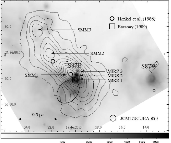
Figure 1: JCMT/SCUBA 850 $\mu$m continuum emission (contours) overlaid on the Spitzer/IRAC 8.0 $\mu$m image. The contour levels increase from 0.6 to 5.0 Jy beam^-1, in a step of 0.4 Jy beam^-1 (4$\sigma$). The inverse grey-scale 8.0 $\mu$m image is in the unit of MJy sr^-1. The coordinate system is J2000. The two small open circles mark the water masers detected by Henkel et al. (1986). The square denotes the compact H ii region, and the open ellipse indicates the position and rough size of the associated extended centimeter emission (Barsony, 1989). The open circle at the bottom shows the beamwidth of JCMT at 850 $\mu$m. The sub-mm clumps SMM 1, SMM 2, and SMM 3, as well as the NIR clusters S87E and S87W, are labeled. Three 8.0 $\mu$m point sources, named as MIRS 1, MIRS 2, and MIRS 3 in § 3.2, are marked by the arrows.

Fig. 1 displays the 850 $\mu$m scan map (contours) and the Spitzer 8.0 $\mu$m image (inverse grey-scale), in which the NIR clusters S87E and S87W are revealed as two bright MIR nebulae. The strongest peak of 850 $\mu$m is associated with S87E, and two other peaks exist to the northeast of it. We propose that these three 850 $\mu$m peaks are associated with three individual sub-mm clumps. They lie along an axis from southwest to northeast, hereafter labeled as SMM 1, SMM 2, and SMM 3.

We processed the sub-mm maps using the Richardson-Lucy (RL) iteration deconvolution algorithm to moderately enhance the spatial resolutions. As many other deconvolution solutions, this algorithm did not produce uncertainty information of the results. Therefore, we have to note that this process is not targeted to get the most “accurate” deconvolved maps. Our steps of deconvolutions are similar to those described by Smith et al. (2000). The 850 and 450 $\mu$m beam patterns of SCUBA were constructed from the Uranus maps measured in 2003 August. A procedure in Starlink/KAPPA was used to perform the image processing tasks. We avoided the pixels at the edge of sub-mm maps during the iterations due to their low signal-to-noise level.

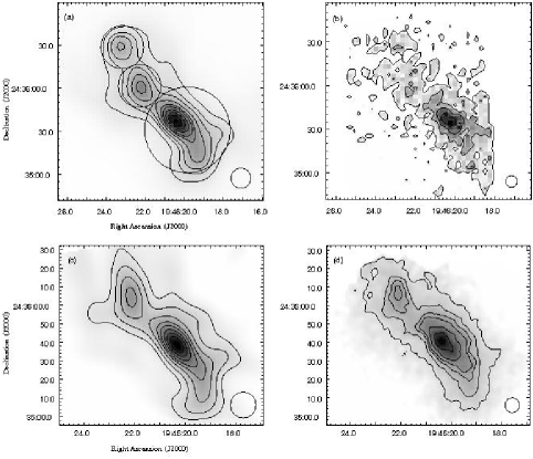
Figure 2: Contour plots of the sub-mm continuum maps, overlaid on their inverse grey-scale images. The beamwidth is indicated in the bottom-right corner of each panel. (a) The deconvolved 850 $\mu$m scan map (M03BU45), after 98 iterations. The contours increase from 1.8 to 29 mJ arcsec^-2 in a step of 3.1 mJ arcsec^-2. The three open circles over the emission peaks denote the photometric apertures (see § 4). (b) The undeconvolved 450 $\mu$m scan map (M03BU45). The contours are: 40, 120, 220, and 380 mJ arcsec^-2. (c) The deconvolved 850 $\mu$m jiggle map (M03AN23), after 51 iterations. The contours increase from 2 to 26 mJ arcsec^-2 in a step of 3 mJ arcsec^-2. (d) The undeconvolved 450 $\mu$m jiggle map (M03AN23). The contours are: 60, 120, 200, 280, 360, 440, and 500 mJ arcsec^-2.

The deconvolutions of the two 850 $\mu$m maps converged within 100 iterations and produced acceptable enhanced maps without apparently artificial structures. However, for the 450 $\mu$m maps, the procedure failed to converge within 150 iterations. Fig. 2 displays the deconvolved 850 $\mu$m maps and undeconvolved 450 $\mu$m maps. All of them have been converted into the units of mJy arcsec^-2. SMM 3 is not covered in the jiggle maps (see Fig. 2c and Fig. 2d) due to the limitation of the observational fields of view. SMM 1 is clearly elongated in the deconvolved 850 $\mu$m maps, and there are extended lobes to the west and south of its peak. SMM 2 is slightly elongated in the north-south direction. All of the three sub-mm clumps are revealed in a common envelop, suggesting that they may be associated although not necessarily in the same sky plane.

To evaluate the CO J = 3 – 2 contribution to the 850 $\mu$m data, we examined our previous observation of S87 in CO J = 3 – 2 at the Köln Observatory for Sub-mm Astronomy (KOSMA) 3m telescope. This observation was carried out for a CO multi-line survey of (UC) H ii regions and has not been published yet (Xue & Wu 2008, in preparation). After converting the integrated intensity of CO J = 3 – 2 to a flux density at 850 $\mu$m, we found that the contribution of CO J = 3 – 2 is less than the noise level of the 850 $\mu$m maps. We also evaluated the contribution of CO J = 6 – 5 to the 450 $\mu$m data by estimating its integrated intensity from CO J = 3 – 2 , under the assumption of local thermodynamic equilibrium (LTE) with an excitation temperature of 80 K. We found that its contribution is also small. Therefore, the effect of line contaminations can be ignored at 450 and 850 $\mu$m.

3.2 Mid/Far-Infrared Images

A luminous MIR point source is revealed at the position of the compact H ii region (see the IRAC images of Fig. 1 and Fig. 3), which we henceforth label as MIRS 1. A weaker MIR point source is found in the 3.6, 4.5, and 5.8 $\mu$m images, $\sim$ 8″ to the southwest of MIRS 1. It is also detected by the 2MASS NIR All-Sky Survey and cataloged as 2MASS 19461947+2435247. However, we did not find the NIR counterpart of MIRS 1 in 2MASS images, indicating that MIRS 1 is highly obscured by the surrounding gas/dust envelope at NIR wavelengths. In the zoomed 8 $\mu$m image of Fig. 1, two other point sources are found to the north of MIRS 1, which we label as MIRS 2 and MIRS 3. Strong diffuse MIR emission exists to the southeast of MIRS 1, coincident with the extended centimeter emission detected by Barsony (1989). Faint diffuse MIR emission is detected in the northeast of the IRAC images, coincident with SMM 3. SMM 2 has no MIR counterpart in all of the IRAC bands.

S87E and S87W saturate the 24 and 70 $\mu$m MIPS images. Five other sources are detected in the 24 $\mu$m band, which are coincident with the diffuse MIR emission in the IRAC bands. We label them as MIRS 4 to MIRS 8 (see Fig. 3). Although the 24 and 70 $\mu$m images are saturated towards SMM 1, it is still clear that the peaks of sub-mm and 24 $\mu$m emission are separate, which is also confirmed by a comparison with the MSX E band (21.3 $\mu$m) image. SMM 3 is associated with MIRS 4. However, its sub-mm peak and MIRS 4 are also slightly separate. There are only weak emission patches in the IRAC 5.8 and 8.0 $\mu$m bands towards SMM 3, indicating that MIRS 4 is still embedded in its gas/dust cocoon. No 24 or 70 $\mu$m emission is detected towards SMM 2, suggesting that it may be less evolved.

3.3 Molecular Lines

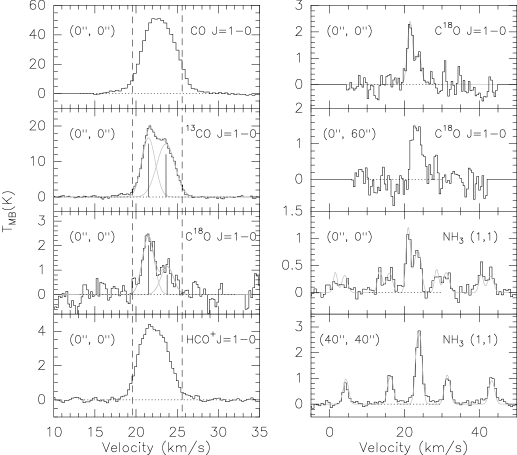
Figure 4: Left panel: The spectra of CO J = 1 – 0 , ¹³CO J = 1 – 0 , C¹⁸O J = 1 – 0 , and HCO⁺ J = 1 – 0 at the reference coordinates: R.A. (J2000) = 19^h46^m19^s.9, Dec. (J2000) = +24°35′24″. The vertical dashed lines define the border of the C¹⁸O J = 1 – 0 emission above 3$\sigma$ level. Right panel: The C¹⁸O J = 1 – 0 spectra from our observation and the NH₃ (J, K) = (1, 1) spectra from Zinchenko et al. (1997). The spatial positions of the spectra are denoted in the top-left corners of small plots. The thin lines on the spectra are the fitted results. We performed double Gaussian fitting for the ¹³CO J = 1 – 0 and C¹⁸O J = 1 – 0 spectra. For the NH₃ (J, K) = (1, 1) transition, we used the NH₃ hyperfine structure fitting procedure of GILDAS/CLASS.

The J = 1 – 0 transitions of CO, ¹³CO, and HCO⁺ exhibit asymmetric line profiles (see the left panel of Fig. 4), and two components are detected in C¹⁸O J = 1 – 0 . Since C¹⁸O J = 1 – 0 is usually optically thin, we can rule out the possibility that the asymmetric line profile in the other transitions is caused by the self-absorption in an infall envelope (Myers et al., 1996; Wu et al., 2005). Previous observations of Stutzki et al. (1984) and Zinchenko et al. (1997) also detected two separate components in NH₃ (J, K) = (1, 1) and NH₃ (J, K) = (2, 2) lines. The NH₃ (J, K) = (1, 1) spectra of Zinchenko et al. (1997) and our C¹⁸O J = 1 – 0 spectra at several positions are plotted in the right panel of Fig. 4. These spectra further confirm that the broad lines of CO J = 1 – 0 , ¹³CO J = 1 – 0 , and HCO⁺ J = 1 – 0 consist of two components.

We fitted our spectra at the reference position with Gaussian profiles. The results are displayed as the thin lines in Fig. 4, and the corresponding derived parameters are summarized in Table 2, including: the line center velocities, the fitted line widths, and the brightness temperatures. We estimated the beam-averaged column densities of C¹⁸O at the reference position using the standard LTE method. The excitation temperature of each component is assumed to be 35 K, in agreement with the estimation from CO J = 1 – 0 (assuming it is optically thick). The derived C¹⁸O column densities are $\sim$ 7.8$\times 10^{15}$ and 4.0$\times 10^{15}$ cm^-2 for the components at low and high velocities.

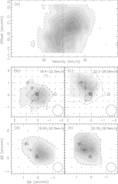
Figure 5: In each plot, the dashed contour denotes the 3$\sigma$ level. The center reference coordinates are: R.A. (J2000) = 19^h46^m19^s.9, Dec. (J2000) = +24°35′24″. (a): The HCO⁺ J = 1 – 0 position-velocity diagram along the northeast-southwest direction. The contour levels increase from 3$\sigma$ to 21$\sigma$ by 3$\sigma$. The vertical dashed line indicates the border of two integrated intervals (see in § 3.3). (b) and (c): The integrated intensity maps of HCO⁺ J = 1 – 0 . The integrated interval is showed in the top-right corner of each plot. The contour levels increase from 40% to 100% by 15% (5$\sigma$) of the peak value. The square denotes the compact H ii region, and the open ellipse indicates the position and rough size of the associated extended centimeter emission (Barsony, 1989). The crosses denote the 850 $\mu$m peaks, and the beamwidth is indicated in the bottom-right corner of each plot. The dashed line is the location of the potential contact plane mentioned in § 5.1. The position of S87W is marked by triangles. (d) and (e): The integrated intensity maps of NH₃ (J, K) = (1, 1) . The contour levels increase from 3$\sigma$ in a step of 3$\sigma$. The spectra data are from Zinchenko et al. (1997). The positions of MIRS 1 and MIRS 4 are marked as triangles.

Fig. 5a is the HCO⁺ J = 1 – 0 position-velocity diagram along the northeast-southwest direction, which also exhibits two components. One is located at the reference position and associated with SMM 1; the other extends from the reference position to the northeast, coincident with SMM 2 and SMM 3. We propose that these components arise from two clouds. Hereafter, they are named Cloud I and II, corresponding with the components at low and high velocity respectively.

The integrated intensity maps of HCO⁺ J = 1 – 0 and NH₃ (J, K) = (1, 1) are also exhibited in Fig. 5. Two different integrated intervals are adopted, chosen to separate the emission from Cloud I and II. All of the presented intensity maps suggest: SMM 2, SMM 3, and the northeast part of SMM 1 may be associated with Cloud II; the main part of SMM 1 is contributed by Cloud I.

4 SED ANALYSIS

4.1 Observational SEDs

We extracted the 850 and 450 $\mu$m flux densities of each clump using a photometric procedure in the Starlink/GAIA software package. The measured results, as well as the positions and sizes of the adopted photometric apertures, are summarized in Table 3. We note that the uncertainties in Table 3 are just statistical errors (rms deviations derived from clean regions), and the estimation of the overall photometric uncertainties is difficult due to the limited information from the online data archives. However, a comparison among different observational modes and the previous similar observation may provide an evaluation of the accuracy of our results.

Jenness et al. (1995) observed S87 using the receiver UKT14 at JCMT in 1994. They detected two sources, which were coincident with SMM 1 and SMM 2 respectively. Our photometric results at 850 $\mu$m are in good agreement with theirs (see the last two columns of Table 3), but the 450 $\mu$m results from SCUBA are systematically larger. Since UKT14 is a single-element bolometer and its measurements may be affected by the change of sky conditions and other factors, we believe that the calibration of SCUBA data is more reliable. The photometric differences of the jiggle and scan maps are acceptable, less than 20% at 450 $\mu$m.

We examined the CSO map and the MIPS images to measure the flux densities of each clump at 24, 70 and 350 $\mu$m. Since SMM 1 saturates the 24 and 70 $\mu$m images, only lower limits can be derived at these wavelengths. In addition, we checked the MSX PSC and found that the photometric apertures of SMM 1 and SMM 3 are coincident with the MSX point sources MSX6C G060.8828-00.1295 and MSX6C G060.9049-00.1275 respectively. Their flux densities are also adopted to construct the SEDs of SMM 1 and SMM 3.

The measured flux densities are summarized in Table 4, extending from sub-mm to MIR. The average results of the scan and jiggle maps are adopted for 850 and 450 $\mu$m. Their differences are considered as the uncertainties. The 350 $\mu$m uncertainties follow the description of Mueller et al. (2002) and the uncertainties at 24 and 70 $\mu$m are the statistical errors.

4.2 Isothermal Dust Model

A simple isothermal gray-body dust model is used to fit the observational SEDs. The details follow the method described by Schnee et al. (2007). In the adopted model, the mean weight of interstellar materials per hydrogen molecule $\mu$ is $\sim$ 2.33. The dust opacity (mass absorption coefficient) $\kappa_{\lambda}$ is dependent on the wavelength and can be described using the equation:

$$\kappa_{\lambda}=\kappa_{1300}(\frac{1300\,\mu\rm m}{\lambda})^{\beta},$$ (1)

where $\beta$ is the dust opacity index and $\kappa_{1300}$ is the dust opacity at 1300 $\mu$m. Assuming a gas-to-dust ratio of 100, we adopt $\kappa_{1300}=0.009\,$cm² g^-1, which is derived from a gas/dust model with thin ice mantles (Ossenkopf & Henning, 1994).

We used a non-linear least-squares method (the Levenberg-Marquardt algorithm coded within IDL) to obtain the best-fit models for the observational SEDs. The physical properties of each sub-mm clump were obtained, including: the average dust temperature $T_{\rm d}$, the dust opacity index $\beta$, and the aperture-average column density of hydrogen molecules $N_{\rm H_{2}}$. In this fitting test, only the data upwards 70 $\mu$m were used. We assumed the 70 $\mu$m flux density of SMM 1 to be 4000 Jy, which was estimated from the interpolation of the IRAS flux densities subtracted with the potential contributions from SMM 2 and SMM 3.

Fig. 6 displays the best-fit model SEDs for three clumps. We further calculated their clump masses and bolometric luminosities $L_{\rm SED}$ (by integrating the model SEDs over the range 1 $\mu$m$<\lambda<2.0$ mm). All of these derived results are summarized in Table 5. Additionally, we adopted a Monte Carlo method used by Schnee et al. (2007) to estimate the errors of the derived parameters that arise from the observational uncertainties. The 3$\sigma$ intervals are denoted as the superscripts and subscripts in Table 5.

The results in Table 5 show that the sub-mm clumps are all massive (110 — 220 $M_{\odot}$). SMM 1 has a higher dust temperature, and its bolometric luminosity dominates in the whole region, implying the existence of strong internal heating source(s). The fitted dust opacity indices of three sub-mm clumps are slightly different ($\sim$ 1.3 — 1.8) and consistent with the typical values between 1 and 2 (Hill et al., 2006). It must be noted that the derived $N_{\rm H_{2}}$ is directly affected by the adopted value of $\kappa_{1300}$. If we reduce $\kappa_{1300}$ by a factor of 2, $N_{\rm H_{2}}$ and the derived clump mass $M$, will increase by a factor of 2. However, the other derived parameters will not be affected by this change.

4.3 Two-temperature Dust Model

In Fig. 6, the best-fit models of SMM 1 and SMM 3 failed to describe the observational results below 70 $\mu$m. However, the model SED of SMM 2 can explain the absence of its MIR emission. To better characterize the excess MIR emission of SMM 1 and SMM 3, we performed another SED fitting test using a model with two dust components at different temperatures. In this fitting test, we adopted the observational data upwards 14.7 $\mu$m (excluding 24 $\mu$m for SMM 1). To reduce the fitting parameters, we assumed $\beta$ is 1.5 and 1.3 for each dust component of SMM 1 and SMM 3 respectively. The best-fit model SEDs are exhibited in Fig. 7, and the derived parameters of the warm and cool dust components are listed in Table 6.

The two-temperature model fits the observational data very well above 12 $\mu$m, which is consistent with the physical fact that there are warm dust around the internal heating sources and relatively cool dust envelopes surrounding the star-forming sites in SMM 1 and SMM 3. Although the IRAS 100 $\mu$m flux density exceeds the model SED of SMM 1 (see Fig. 7), we believe that the deviation is due to the large beam of IRAS . The results in Fig. 7 and Table 6 show that the warm components contribute little to the total masses and the flux densities at sub-mm wavelengths, but are required to explain the excess at MIR wavelengths.

We tried to modify $\beta$ to fit the emission below 12 $\mu$m. However, no satisfying results were found. The emission in the MSX A and C bands does not follow the predication of gray-body models, suggesting these models are invalid at these wavelengths. Generally, two significant spectral features may exist at this MIR wavelength range. One is the emission of polycyclic aromatic hydrocarbons (PAHs), which is often detected towards compact H ii regions and photodissociation regions (PDRs). Previous studies have showed that the MSX A and C bands often contain PAH emission lines (Ghosh & Ojha, 2002; Kraemer et al., 2003a; Povich et al., 2007). The other is the silicate feature, which has been predicted in the dust model of Ossenkopf & Henning (1994) and demonstrated to be important in the recent sophisticated SED models (Robitaille et al., 2006, 2007). This feature may be expected as the absorption at 9.7 $\mu$m towards some UC H ii regions, produced by the dust cocoons around center objects (Faison et al., 1998). Peeters et al. (2002) have identified both of PAH and silicate features towards S87E in the previous ISO spectroscopy observation. The silicate absorption feature may be caused by Cloud II, which partly overlaps above the compact H ii region. Since our gray-body models are focused to evaluate the overall properties of dust clumps, which are mainly constrained by the thermal emission from longer wavelengths, a detailed SED model explaining the PAH and silicate features is beyond our purpose.

5 DISCUSSION

5.1 Cloud-Cloud Collision

All of the FIR/sub-mm images and molecular line maps exhibit the complex spatial and kinematical structures of S87. The recently published high-resolution C¹⁸O J = 1 – 0 observation (Saito et al., 2007) revealed several gas clumps at different velocities, which further confirms our identification of Cloud I and II. However, are Cloud I and II really related to each other? Saito et al. (2007) proposed that the gas clumps at higher velocity might be on the near side along the line-of-sight because the observation of Chen et al. (2003) detected many reddened sources in NIR there. They further reasoned that the clumps at low and high velocities were approaching and the NIR cluster S87E was possibly formed by a cloud-cloud collision. In the following, we verify the cloud-cloud collision model by a multi-wavelength comparison.

Firstly, the 8.0 $\mu$m emission shows a sharp edge to the northeast of MIRS 1 (see Fig. 1). This feature is probably caused by the large extinction at 8.0 $\mu$m because the sub-mm emission is still strong. The position of the extinction patch is consistent with that of Cloud II, confirming that Cloud II is on the near side along the line-of-sight. Therefore, Cloud I and II are approaching.

Next, we can infer from the intensity maps of Fig. 5 that the peak of SMM 1 and S87E are in the overlapping region of Cloud I and II. The MIR point sources in SMM 1 suggest that there is not only a formed NIR cluster, but also ongoing star-forming activities. The strong and continuous star-forming process is likely to be interpreted by the stimulation of a cloud-cloud collision rather than the spontaneous evolution of molecular clouds alone.

Furthermore, the spatial configuration of the compact H ii region and the associated extended centimeter emission (Barsony, 1989; Kurtz et al., 1994) also supports the cloud-cloud collision model. The champagne flow model of Kim & Koo (2001) combined with clumpy structures of molecular clouds can explain the extended centimeter component which stretches to the southeast of the compact H ii region. If Cloud I and II are in contact, their contact plane will be along the northwest-southeast direction (see Fig. 5b and Fig. 5c). Consequently, the compact H ii region will be better confined in the direction perpendicular to the contact plane and the champagne flow should be easier to spurt out in the southeast direction. If Cloud I and II are not in contact, the champagne flow will be more likely to splash in the direction perpendicular to the border of the parent cloud of the compact H ii region. The observational result is consistent with the predication of the first scenario, supporting that the two clouds are colliding. Assuming that the two clouds have typical sizes $R$ $\sim$ 1 pc and a velocity separation $\delta v$ $\sim$ 2 km s^-1, the collision duration is at least $R/\delta v\sim 5\times 10{{}^{5}}$ yrs, comparable with the time scale forming a compact H ii region.

The cloud-cloud collision is considered as an efficient mechanism to trigger star formation. It may compress molecular gas and lead to local gravitational collapse (Loren, 1976; Habe & Ohta, 1992; Marinho et al., 2001). However, its possibility is small in the diffuse molecular clouds (Elmegreen, 1998). Additionally, high velocity off-axis collisions could be destructive rather than lead to gravitational instabilities (Hausman, 1981; Gilden, 1984). Therefore, the fraction of star formation triggered by cloud-cloud collisions may be small in our Galaxy. All of the current evidence demonstrates that S87 is a new example of cloud-cloud collisions, and similar samples are still limited (Loren, 1976; Dickel et al., 1978; Koo et al., 1994; Vallee, 1995; Buckley & Ward-Thompson, 1996; Sato et al., 2000; Looney et al., 2006).

5.2 Molecular Line Emission

5.2.1 HCO⁺ J = 1 – 0

Our observation shows that the line profile of HCO⁺ J = 1 – 0 is similar to that of CO J = 1 – 0 (see the left panel of Fig. 4). Additionally, we found that both of CO J = 1 – 0 and HCO⁺ J = 1 – 0 spectra show slight features of high-velocity (HV) gas when compared with C¹⁸O J = 1 – 0 , suggesting that HCO⁺ extends in diffuse gas rather than simply concentrates in the dense parts of gas clumps. Previous observational and theoretical works have pointed out the abundance enhancement of HCO⁺ in diffuse or shocked gas (Turner, 1995b; Girart et al., 1999), which can explain our finding.

However, the formation mechanism of the HV gas in S87 is unclear. We propose three different explanations: (i) the HV gas may arise from stellar outflows; (ii) it may be contributed by the high-pressure shocked material that is squirted out when the clouds collide; (iii) or, it is from the non-impacting portions of the colliding clouds since they do not slow down to a common speed during the cloud-cloud collision. Although Barsony (1989) identified HV blue and red wings in her CO J = 1 – 0 observation and proposed that the HV gas resulted from a biconical outflow with a wide opening angle viewed at large inclination, our identification of two individual clouds apparently rejects this model. High-resolution and sensitive observations are required to clarify the origin of the HV gas.

Because both stellar outflows and cloud-cloud collisions can produce HV gas and broad non-Gaussian line profiles, it is possible that some observational results previously interpreted as bipolar outflows are caused by cloud-cloud collisions. However, since the possibility of cloud-cloud collisions is not high, similar cases like S87 should be rare.

5.2.2 NH₃ (J, K) = (1, 1)

A feature of the NH₃ (J, K) = (1, 1) intensity maps is that the NH₃ emission tends to “evade” the luminous MIR sources. The NH₃ (J, K) = (1, 1) peak of Cloud I is separate from MIRS 1 and the sub-mm peak of SMM 1. The NH₃ (J, K) = (1, 1) emission is absent to the southeast of MIRS 1, where the diffuse MIR emission is strong. The NH₃ (J, K) = (1, 1) peak of Cloud II is coincident with SMM 2, which has no MIR counterpart. In contrast, the observations of Saito et al. (2007) and Shirley et al. (2003) showed that the C¹⁸O J = 1 – 0 and CS J = 5 – 4 emission is strong in SMM 1 and SMM 3. Since both of SMM 1 and SMM 3 are dense clumps identified from sub-mm continuum, their relatively weak NH₃ emission may be explained by the underabundance of NH₃. Turner (1995a) suggested that NH₃ could be destroyed by C⁺ that dominates in PDRs. However, molecules like C¹⁸O are formed via C⁺ and not affected by the photo-destruction process (Jansen et al., 1995). The diffuse 5.8 and 8.0 $\mu$m emission near SMM 1 and SMM 3 is usually contributed by PAHs and interpreted as a tracer of PDRs. The existence of MIR emission there, as well as the strong C¹⁸O J = 1 – 0 emission and the weak NH₃ emission, are consistent with the prediction of the chemical process proposed in previous works.

5.2.3 virial States

The line widths of molecular spectra are usually used to probe the kinematics of gas clumps. Since Cloud I and II can be well resolved in NH₃ lines, we estimate the virial masses of these two clouds in this section.

We derived the line widths and brightness temperatures of NH₃ (J, K) = (1, 1) at the NH₃ peaks of Cloud I and II, using the hyperfine structure fitting procedure of GILDAS/CLASS. The results are exhibited as thin lines in Fig. 4. The angular diameters $\theta_{\rm obs}$ of Cloud I and II are calculated using the equation:

$$\theta_{\rm obs}=2\sqrt{\frac{\Omega}{\pi}},$$ (2)

in which, $\Omega$ is the measured angular area of each cloud. After that, we corrected the beam effect and estimated the intrinsic sizes of Cloud I and II following the equation:

$$R=D\frac{\sqrt{\theta_{\rm obs}^{2}-\theta_{\rm mb}^{2}}}{2},$$ (3)

where $R$ is the radius of the gas cloud in pc, $D$ is the distance of S87, and $\theta_{\rm mb}$ is the beamwidth of the NH₃ (J, K) = (1, 1) observation. Assuming that Cloud I and II are homogeneous spherical gas clouds with a density distribution $\rho\propto r^{-\alpha}$ ($\alpha=1.5$) and neglecting the contributions from magnetic field and surface pressure, the virial masses can be derived using the equation (MacLaren et al., 1988):

$$M_{\rm vir}=126(\frac{5-2\alpha}{3-\alpha})R\Delta V_{\rm FWHM}^{2},$$ (4)

in which, $M_{\rm vir}$ is the virial mass in $M_{\odot}$ and $\Delta V_{\rm FWHM}$ is the full width at half-maximum intensity (FWHM) of NH₃ (J, K) = (1, 1) in km s^-1.

All the measured and derived parameters of Cloud I and II are listed in Table 7, including: the positions of NH₃ peaks, the angular and intrinsic sizes, the line widths at NH₃ peaks, and the derived virial masses of two clouds. The total virial mass of Cloud I and II is $\sim$ 430 $M_{\odot}$, which is much smaller than the previous estimation ($\sim$ 1080 $M_{\odot}$) obtained with the total line width of two components (Zinchenko et al., 1997) but comparable with the mass estimated from the SED fitting ($\sim$ 460 $M_{\odot}$, from the isothermal dust model). However, we note that the above comparison of the masses estimated from different approaches can be affected by the adopted dust opacity and the assumption of $\alpha$. Although a variation of $\alpha$ is not likely to cause much change in virial masses, the dust opacity may change by at least a factor of 2 (Ossenkopf & Henning, 1994), which leads to a large uncertainty in the masses estimated from SEDs.

5.3 Stellar Contents of SMM 1 and SMM 3

The position of MIRS 1 is consistent with that of the compact H ii region, within the astrometric error (1.5″), indicating that MIRS 1 is the exciting massive (proto)star. We examined the high-resolution centimeter map of Barsony (1989) and found that neither MIRS 2 nor MIRS 3 shows compact radio continuum emission. The possible explanation is that MIRS 2 and MIRS 3 are less evolved compared with MIRS 1 or they are not massive enough to ionize their surroundings and to excite compact H ii regions. Henkel et al. (1986) detected a strong water maser in SMM 1, which is often considered to be associated with HMPOs. The velocity range of this water maser is 21 — 25 km s^-1, in good agreement with the systematic velocity of the molecular clouds. All the evidence mentioned above supports that SMM 1 is a high-mass star-forming site that harbors massive forming stars or cluster.

The Lyman continuum radiation from massive stars mainly escapes in the form of free-free emission. Kurtz et al. (1994) estimated that the Lyman continuum photon flux required to keep the entire region of S87E ionized was $3.2\times 10^{46}$ photons s^-1, which corresponds to that of a B0.5 ZAMS star. The bolometric luminosity of such stars is $\sim$ $3.0\times 10^{4}$ $L_{\odot}$ (Crowther, 2005), slightly smaller than that of SMM 1 ($\sim$ $3.7\times 10^{4}$$L_{\odot}$, from the two-component model). The extra luminosity of SMM 1 may come from the relatively weak MIR sources near MIRS 1, which can not be traced by the free-free emission.

SMM 3 contains the bright 24 $\mu$m source MIRS 4. The ratio of the luminosities from its cool and warm components is $\sim$ 2.1, lower that of SMM 1. Its bolometric luminosity is $\sim$ 740 $L_{\odot}$, also lower than that of SMM 1, which indicates that SMM 3 is more likely to be an intermediate-mass star-forming site.

5.4 Physical Properties of SMM 2

No MIR point source or diffuse emission below 70 $\mu$m is detected towards SMM 2. Since only a cold dust component can describe its observational SED, strong internal heating sources are not likely to exist in SMM 2.

Henkel et al. (1986) detected a weak 22 GHz water maser near SMM 2, which usually arises from the dense circumstellar disks around protostars (Park & Choi, 2007) or originates in outflows from the birth of a massive star (van Dishoeck & Blake, 1998). Since this water maser is in the velocity range 8 — 15 km s^-1, significantly different from that of the molecular clouds, we favor the second explanation for its origin. We notice that this water maser is on a sub-mm emission ridge connecting the peaks of SMM 1 and SMM 2 rather than near the peak of SMM 2, and its position uncertainty is large when compared with sub-mm observations. Therefore, we doubt that this weak maser is produced by the intrinsic factors of SMM 2. For instance, the potential outflows from massive protostars of SMM 1 may shock the ambient molecular gas of SMM2 and produce a weak water maser at the rear side of SMM2. This scenario is consistent with the lower velocity of the water maser. Therefore, we believe that the existence of this water maser does not necessarily contradict SMM 2’s physical properties derived from the SED and MIR image analyses. Based on the information available, we support that SMM 2 is probably a HMSC that may form massive stars or intermediate star clusters eventually.

6 CONCLUSIONS

We have carried out a multi-wavelength study of the massive star-forming region S87. The main results are summarized as follows.

1. We identified three sub-mm clumps in S87, labeled as SMM 1, SMM 2, and SMM 3. They are estimated to have masses of 210, 140, and 110 $M_{\odot}$, with average dust temperatures of 41, 21, and 24 K respectively (from the isothermal gray-body model).

2. We examined molecular line maps from our observations and compared them with previous results of other authors. We concluded that the star-forming activities in SMM 1 are stimulated by a cloud-cloud collision.

3. We found that HCO⁺ can trace diffuse gas and NH₃ may be destructed by chemical processes in the region harboring MIR sources or exhibiting strong diffuse MIR emission.

4. We calculated the virial masses of the two colliding clouds, which are in good agreement with those estimated from SEDs.

5. The stellar contents and star-forming activities of sub-mm clumps are identified. Their SEDs reveal that these clumps are at various evolutionary stages. SMM 1 and SMM 3 are high-mass and intermediate-mass star-forming regions respectively. SMM2 is massive and cold, has no MIR counterpart, which is probably a HMSC. All of these results expose that the star formation in S87 is at multiple phases.

Table 1: Observation Parameters

Transition	$\nu_{\rm rest}$	HPBW	Bandwidth	$\Delta V_{\rm res}$	1$\sigma$ rmsa
	(GHz)	(″)	(MHz)	(km s-1)	(K chan.-1)
CO J = 1 – 0	115.271204	46	145	0.37	0.18
13CO J = 1 – 0	110.201353	47	43	0.11	0.14
C18O J = 1 – 0	109.782182	48	43	0.12	0.14
HCO+ J = 1 – 0	89.188521	58	43	0.26	0.11

Table 2: Parameters of Molecular Lines

Transitiona	$V_{\rm LSR}$	$\Delta V$	$T_{\rm mb}$
	(km s-1)	(km s-1)	(K)
13CO J = 1 – 01	21.51 (0.08)	1.93 (0.04)	16.71 (0.38)
C18O J = 1 – 01	21.48 (0.08)	1.69 (0.19)	2.39 (0.39)
13CO J = 1 – 02	23.61 (0.04)	2.60 (0.06)	15.04 (0.38)
C18O J = 1 – 02	23.78 (0.16)	1.83 (0.42)	1.14 (0.39)
HCO+ J = 1 – 0b	22.30 (0.04)	3.10 (0.16)	4.54 (0.11)

Table 3: Photometric Results of the Sub-mm Clumps

Object	$\alpha$	$\delta$	$\theta_{\rm ap}$	850 $\mu$ma	450 $\mu$ma	850 $\mu$mb	450 $\mu$mb	850 $\mu$mc	450 $\mu$mc
	J2000	J2000	(″)	(Jy)	(Jy)	(Jy)	(Jy)	(Jy)	(Jy)
SMM 1	19 46 19.8	+24 35 32	60	17.7$\pm$0.1	133$\pm$10	16.8$\pm$0.1	167$\pm$1	17	110
SMM 2	19 46 22.3	+24 36 01	30	5.8$\pm$0.1	32$\pm$6	5.3$\pm$0.1	45$\pm$1	6.5	18
SMM 3	19 46 23.2	+24 36 28	30	4.1$\pm$0.1	25$\pm$6	—	—	—	—

Table 4: Flux Densities of the Sub-mm Clumps

Object	850 $\mu$m	450 $\mu$m	350 $\mu$m	70 $\mu$m	24 $\mu$m	21.3 $\mu$ma	14.7 $\mu$ma	12.1 $\mu$ma	8.3 $\mu$ma
	(Jy)	(Jy)	(Jy)	(Jy)	(Jy)	(Jy)	(Jy)	(Jy)	(Jy)
SMM 1	17.3$\pm$0.9	150$\pm$34	256$\pm$46	$>1500^{\rm b}$	$>24^{\rm b}$	225$\pm$13	43.3$\pm$2.3	31.7$\pm$1.6	19.6$\pm$0.8
SMM 2	5.5$\pm$0.6	39$\pm$13	79$\pm$14	49$\pm$3	$<3^{\rm c}$	—	—	—	—
SMM 3	4.1$\pm$0.6	25$\pm$6	40$\pm$8	36$\pm$3	9.1$\pm$3.0	5.1$\pm$0.4	0.6$\pm$0.1	1.1$\pm$0.1	1.3$\pm$0.1

Table 5: Best-fit Parameters for the SEDs (I)

Object	$T_{\rm d}$	$\beta$	${N_{\rm H_{2}}}^{\rm a}$	$M$	${L_{\rm SED}}^{\rm b}$
	(K)		(1022 cm-2)	($M_{\odot}$)	($L_{\odot}$)
SMM 1	41${}^{+9}_{-5}$	1.5${}^{+0.3}_{-0.4}$	3.2${}^{+0.9}_{-0.5}$	210${}^{+60}_{-40}$	31000
SMM 2	21${}^{+2}_{-1}$	1.8${}^{+0.3}_{-0.3}$	8.4${}^{+0.6}_{-0.5}$	140${}^{+20}_{-30}$	1100
SMM 3	24${}^{+2}_{-2}$	1.3${}^{+0.3}_{-0.2}$	6.4${}^{+0.6}_{-0.5}$	110${}^{+30}_{-30}$	600

Table 6: Best-fit Parameters for the SEDs (II)

Object	$T_{\rm d}$	$\beta$	${N_{\rm H_{2}}}^{\rm a}$	$M$	${L_{\rm SED}}^{\rm b}$
— component	(K)		(1020 cm-2)	($M_{\odot}$)	($L_{\odot}$)
SMM 1— cool	40	1.5	320	210	30000
— warm	92	1.5	0.7	0.5	7200
SMM 3— cool	23	1.3	690	112	500
— warm	82	1.3	0.4	0.1	240

Table 7: Parameters of virial Mass Estimatation

Object	$V_{\rm LSR}$	$\Delta\alpha^{\rm a}$	$\Delta\delta^{\rm a}$	$\Delta V$	$\theta_{\rm obs}$	$R$	$M_{\rm vir}^{\rm b}$
	(km s-1)	(″)	(″)	(km s-1)	(″)	(pc)	($M_{\odot}$)
Cloud I	21.01(0.06)	0	0	1.22(0.15)	126	0.67	170
Cloud II	23.84(0.02)	40	40	1.60(0.05)	116	0.60	260

Figure 3: The Spitzer MIR/FIR images at six wavelengths. The sizes and positions of six panels are the same. The absolute coordinates (J2000) are exhibited in the 8.0 $\mu$m panel. The white areas in the emission regions of 24 and 70 $\mu$m images are due to the saturation of the detectors. The MIR emission is also plotted as contours in the 3.6, 4.5, 5.8, and 8.0 $\mu$m panels. Their contour levels are: 1%, 2%, 3%, 5%, 10%, 16%, 28%, 50%, and 90% of the peak intensities. The crosses in each panel denote the 850 $\mu$m peaks. The square indicates the compact H ii region. The contour plot of the 24 $\mu$m panel is the 850 $\mu$m continuum emission, adopted from Fig. 2a. MIRS 4 to MIRS 8 are also marked in the 24 $\mu$m panel. The small open circles in the bottom-right corner of 24 and 70 $\mu$m panels denote the resolutions of these observations.

Figure 6: From (a) to (c), the best-fit SEDs (solid lines) of SMM 1, SMM 2, and SMM 3 are exhibited. The filled triangles denote the flux densities of IRAS 19442+2427. The open triangles denote the flux densities extracted from MSX PSC. The open squares indicate the flux densities derived from the Spitzer/MIPS images. The small filled squares on the model SEDs are the data points used for the SED fitting. The errorbar of each data point is plotted if available.

Figure 7: The panel (a) and (b) exhibit the best-fit SEDs of SMM 1 and SMM 3 (solid lines). The two components of model SEDs are also displayed (dot lines) respectively. The filled triangles denote the flux densities of IRAS 19442+2427. The open triangles denote the flux densities extracted from MSX PSC. The open squares indicate the flux densities derived from the Spitzer/MIPS images. The small filled squares on the model SEDs are the data points used for the SED fitting. The errorbar of each data point is plotted if available.

References

- Bally & Predmore (1983) Bally, J., & Predmore, R. 1983, ApJ, 265, 778
- Barsony (1989) Barsony, M. 1989, ApJ, 345, 268
- Benjamin et al. (2003) Benjamin, R. A., et al. 2003, PASP, 115, 953
- Beuther et al. (2002) Beuther, H., Schilke, P., Menten, K. M., Motte, F., Sridharan, T. K., & Wyrowski, F. 2002, ApJ, 566, 945
- Beuther et al. (2007) Beuther, H., Churchwell, E. B., McKee, C. F., & Tan, J. C. 2007, Protostars and Planets V, 165
- Beuther & Steinacker (2007) Beuther, H., & Steinacker, J. 2007, ApJ, 656, L85
- Buckley & Ward-Thompson (1996) Buckley, H. D., & Ward-Thompson, D. 1996, MNRAS, 281, 294
- Carey et al. (2005) Carey, S. J., et al. 2005, Bulletin of the American Astronomical Society, 37, 1252
- Chen et al. (2003) Chen, Y., Zheng, X.-W., Yao, Y., Yang, J., & Sato, S. 2003, A&A, 401, 185
- Churchwell (2002) Churchwell, E. 2002, ARA&A, 40, 27
- Crampton et al. (1978) Crampton, D., Georgelin, Y. M., & Georgelin, Y. P. 1978, A&A, 66, 1
- Crowther (2005) Crowther, P. A. 2005, Massive Star Birth: A Crossroads of Astrophysics, 227, 389
- Dickel et al. (1978) Dickel, J. R., Dickel, H. R., & Wilson, W. J. 1978, ApJ, 223, 840
- Egan et al. (2003) Egan, M. P., Price, S. D., & Kraemer, K. E. 2003, Bulletin of the American Astronomical Society, 35, 1301
- Elmegreen (1998) Elmegreen, B. G. 1998, Origins, 148, 150
- Faison et al. (1998) Faison, M., Churchwell, E., Hofner, P., Hackwell, J., Lynch, D. K., & Russell, R. W. 1998, ApJ, 500, 280
- Fazio et al. (2004) Fazio, G. G., et al. 2004, ApJS, 154, 10
- Forbrich et al. (2004) Forbrich, J., Schreyer, K., Posselt, B., Klein, R., & Henning, T. 2004, ApJ, 602, 843
- Garay et al. (2004) Garay, G., Faúndez, S., Mardones, D., Bronfman, L., Chini, R., & Nyman, L.-Å. 2004, ApJ, 610, 313
- Ghosh & Ojha (2002) Ghosh, S. K., & Ojha, D. K. 2002, A&A, 388, 326
- Gilden (1984) Gilden, D. L. 1984, ApJ, 279, 335
- Girart et al. (1999) Girart, J. M., Ho, P. T. P., Rudolph, A. L., Estalella, R., Wilner, D. J., & Chernin, L. M. 1999, ApJ, 522, 921
- Guilloteau & Lucas (2000) Guilloteau, S. & Lucas, R. 2000, in Imaging at Radio through Submillimeter Wavelengths, eds. J.G. Mangum & S. Radford, ASP Conf. Ser., 217, 299
- Habe & Ohta (1992) Habe, A., & Ohta, K. 1992, PASJ, 44, 203
- Hausman (1981) Hausman, M. A. 1981, ApJ, 245, 72
- Henkel et al. (1986) Henkel, C., Guesten, R., & Haschick, A. D. 1986, A&A, 165, 197
- Hill et al. (2006) Hill, T., Thompson, M. A., Burton, M. G., Walsh, A. J., Minier, V., Cunningham, M. R., & Pierce-Price, D. 2006, MNRAS, 368, 1223
- Holland et al. (1999) Holland, W. S., et al. 1999, MNRAS, 303, 659
- Hunter et al. (2000) Hunter, T. R., Churchwell, E., Watson, C., Cox, P., Benford, D. J., & Roelfsema, P. R. 2000, AJ, 119, 2711
- Jansen et al. (1995) Jansen, D. J., van Dishoeck, E. F., Black, J. H., Spaans, M., & Sosin, C. 1995, A&A, 302, 223
- Jenness et al. (1995) Jenness, T., Scott, P. F., & Padman, R. 1995, MNRAS, 276, 1024
- Jenness et al. (2002) Jenness, T., Stevens, J. A., Archibald, E. N., Economou, F., Jessop, N. E., & Robson, E. I. 2002, MNRAS, 336, 14
- Kim & Koo (2001) Kim, K.-T., & Koo, B.-C. 2001, ApJ, 549, 979
- Koo et al. (1994) Koo, B.-C., Lee, Y., Fuller, G. A., Lee, M. G., Kwon, S.-M., & Jung, J.-H. 1994, ApJ, 429, 233
- Kraemer et al. (2003a) Kraemer, K. E., Shipman, R. F., Price, S. D., Mizuno, D. R., Kuchar, T., & Carey, S. J. 2003, AJ, 126, 1423
- Kraemer et al. (2003b) Kraemer, K. E., et al. 2003, ApJ, 588, 918
- Kurtz et al. (1994) Kurtz, S., Churchwell, E., & Wood, D. O. S. 1994, ApJS, 91, 659
- Kutner & Ulich (1981) Kutner, M. L., & Ulich, B. L. 1981, ApJ, 250, 341
- Looney et al. (2006) Looney, L. W., Wang, S., Hamidouche, M., Safier, P. N., & Klein, R. 2006, ApJ, 642, 330
- Loren (1976) Loren, R. B. 1976, ApJ, 209, 466
- MacLaren et al. (1988) MacLaren, I., Richardson, K. M., & Wolfendale, A. W. 1988, ApJ, 333, 821
- Marinho et al. (2001) Marinho, E. P., Andreazza, C. M., & Lépine, J. R. D. 2001, A&A, 379, 1123
- Molinari et al. (1996) Molinari, S., Brand, J., Cesaroni, R., & Palla, F. 1996, A&A, 308, 573
- Molinari et al. (2002) Molinari, S., Testi, L., Rodríguez, L. F., & Zhang, Q. 2002, ApJ, 570, 758
- Mueller et al. (2002) Mueller, K. E., Shirley, Y. L., Evans, N. J., II, & Jacobson, H. R. 2002, ApJS, 143, 469
- Myers et al. (1996) Myers, P. C., Mardones, D., Tafalla, M., Williams, J. P., & Wilner, D. J. 1996, ApJ, 465, L133
- Ossenkopf & Henning (1994) Ossenkopf, V., & Henning, T. 1994, A&A, 291, 943
- Park & Choi (2007) Park, G., & Choi, M. 2007, ApJ, 664, L99
- Peeters et al. (2002) Peeters, E., et al. 2002, A&A, 381, 571
- Povich et al. (2007) Povich, M. S., et al. 2007, ApJ, 660, 346
- Racine (1968) Racine, R. 1968, AJ, 73, 233
- Rieke et al. (2004) Rieke, G. H., et al. 2004, ApJS, 154, 25
- Robitaille et al. (2006) Robitaille, T. P., Whitney, B. A., Indebetouw, R., Wood, K., & Denzmore, P. 2006, ApJS, 167, 256
- Robitaille et al. (2007) Robitaille, T. P., Whitney, B. A., Indebetouw, R., & Wood, K. 2007, ApJS, 169, 328
- Saito et al. (2007) Saito, H., Saito, M., Sunada, K., & Yonekura, Y. 2007, ApJ, 659, 459
- Sato et al. (2000) Sato, F., Hasegawa, T., Whiteoak, J. B., & Miyawaki, R. 2000, ApJ, 535, 857
- Schnee et al. (2007) Schnee, S., Kauffmann, J., Goodman, A., & Bertoldi, F. 2007, ApJ, 657, 838
- Sharpless (1959) Sharpless, S. 1959, ApJS, 4, 257
- Shirley et al. (2003) Shirley, Y. L., Evans, N. J., II, Young, K. E., Knez, C., & Jaffe, D. T. 2003, ApJS, 149, 375
- Smith et al. (2000) Smith, K. W., Bonnell, I. A., Emerson, J. P., & Jenness, T. 2000, MNRAS, 319, 991
- Sridharan et al. (2002) Sridharan, T. K., Beuther, H., Schilke, P., Menten, K. M., & Wyrowski, F. 2002, ApJ, 566, 931
- Sridharan et al. (2005) Sridharan, T. K., Beuther, H., Saito, M., Wyrowski, F., & Schilke, P. 2005, ApJ, 634, L57
- Stutzki et al. (1984) Stutzki, J., Olberg, M., Winnewisser, G., Jackson, J. M., & Barrett, A. H. 1984, A&A, 139, 258
- Turner (1995a) Turner, B. E. 1995, ApJ, 444, 708
- Turner (1995b) Turner, B. E. 1995, ApJ, 449, 635
- Vallee (1995) Vallee, J. P. 1995, AJ, 110, 2256
- van Dishoeck & Blake (1998) van Dishoeck, E. F., & Blake, G. A. 1998, ARA&A, 36, 317
- Wu et al. (2005) Wu, Y., Zhu, M., Wei, Y., Xu, D., Zhang, Q., & Fiege, J. D. 2005, ApJ, 628, L57
- Wu et al. (2006) Wu, Y., Zhang, Q., Yu, W., Miller, M., Mao, R., Sun, K., & Wang, Y. 2006, A&A, 450, 607
- Zinchenko et al. (1997) Zinchenko, I., Henning, T., & Schreyer, K. 1997, A&AS, 124, 385