The influence of localized states charging on $1/f^{\alpha}$ tunneling current noise spectrum

Abstract

We report the results of theoretical investigations of low frequency tunneling current noise spectra component ($1/f^{\alpha}$). Localized states of individual impurity atoms play the key role in low frequency tunneling current noise formation. It is found that switching ”on” and ”off” of Coulomb interaction of conduction electrons with one or two charged localized states results in power law singularity of low-frequency tunneling current noise spectrum $1/f^{\alpha}$. Power law exponent in different low frequency ranges depends on the relative values of Coulomb interaction of conduction electrons with different charged impurities.

I Introduction

In the present work we discuss one of the possible reasons for the $1/f^{\alpha}$ noise in the STM/STS junctions. We suggest the theoretical model for tunneling current noise above the flat surface and above the impurity atoms on semiconductor or metallic surfaces. We found out that changing of the power law exponent above the flat surface and above the impurity atom depends on the parameters of tunneling junction such as tip-sample separation Oreshkin .

Problem of low frequency noise with $1/f^{\alpha}$ spectra formation in electron devices is one of the most interesting and important in recent years. Usually the typical approach to $1/f^{\alpha}$ noise problem consists of ”by hand” introducing of the random relaxation time $\tau_{0}$ for two-state system with the probability distribution function $A/\tau_{0}^{\alpha}$. Therefore the averaged over $\tau_{0}$ noise spectra of two-states system has power law singularity. But the physical nature and the microscopic origin of such probability distribution function in general is unknown.Up to now only the limited number of works was devoted to the problem of $1/f^{\alpha}$ noise study. The investigations of the noise in two-level system was carried out in Galperin . Authors studied current noise in a double-barrier resonant-tunneling structure due to dynamic defects that switch states because of their interaction with a thermal bath. The time fluctuations of the resonant level result in low-frequency noise, the characteristics of which depend on the relative strengths of the electron escape rate and the defect’s switching rate. If the number of defects is large, the noise is of the $1/f$ type. In Levitov authors studied shot noise in a mesoscopic quantum resistor. They found correlation functions of all order, distribution function of the transmitted charge and considered Pauli principle as the reason for the fluctuations. Altshuler et al. Altshuler studied current fluctuations in a mesoscopic conductor. They derived a general expression for the fluctuations in the cylindrical tunneling contact in the presence of a time dependent voltage. In Moller Moller, Esslinger and Koslowski have investigated the noise of tunneling current at zero bias voltage. The measurements were carried out at UHV conditions at base pressure $5\times 10^{-11}$ torr. The authors have demonstrated that at zero bias voltage the $1/f^{\alpha}$ component of noise in the tunneling current vanishes and white noise becomes dominant. Tiedje et al. Tiedje have found the $1/f^{\alpha}$ dependence of the current noise in STM experiments on graphite in ambient conditions. They attributed this effect to fluctuations induced by adsorbates in tunneling junction area.

In Lozano the fluctuations of tunneling barrier height have been investigated. The experiments have been performed under UHV conditions on graphite and gold samples using PtIr tips. From these measurements the authors have concluded that the intensity of barrier height fluctuations correspond to the intensity of tunneling current $1/f^{\alpha}$ noise in the frequency range from 1 to 100 Hz.

Our aim is to study one of the possible microscopic origins of $1/f^{\alpha}$ noise in tunneling contact. We shall analyse tunneling contact model with localized states and Coulomb interaction between them which gives us opportunity to describe the formation of $1/f^{\alpha}$ tunneling current noise spectra.

II The suggested model and main results

Let’s start from the model of two localized states in tunneling contact. In this case one of the localized states is formed by impurity atom in semiconductor and the other one by tip apex.

When electron tunnels in or from localized state, the electron filling numbers of localized state rapidly change leading to appearance of localized state additional charge and sudden switching ”on” and ”off” Coulomb potential. Electrons in the leads feel this Coulomb potential.

The model system (Fig. 1) can be described by hamiltonian $\hat{H}$:

$$\hat{H}=\hat{H}_{0}+\hat{H}_{tun}+\hat{H}_{int}$$

$$\hat{H}_{0} =\sum_{p}(\varepsilon_{p}-eV)c_{p}^{+}c_{p}+\sum_{k}\varepsilon_{k}c_{k}^{+}c_{k}+\sum_{i=1,2}\varepsilon_{i}a_{i}^{+}a_{i}$$ (1)

$$\hat{H}_{tun} =\sum_{k,i}T_{ki}c_{k}^{+}a_{i}+\sum_{p,i}T_{pi}c_{p}^{+}a_{i}+T\sum a_{1}^{+}a_{2}+h.c.$$

$$\hat{H}_{int} =\sum_{k,k^{{}^{\prime}}}W_{1}c_{k}^{+}c_{k^{{}^{\prime}}}a_{1}a_{1}^{+}+W_{2}c_{k}^{+}c_{k^{{}^{\prime}}}a_{2}a_{2}^{+}\$$

$\hat{H}_{0}$ describes free electrons in the leads and in localized states. $\hat{H}_{tun}$ describes tunneling transitions between the leads through localized states. $\hat{H}_{int}$ corresponds to processes of intraband scattering caused by Coulomb potentials $W_{1}$, $W_{2}$ of localized states charges.

Operators $c_{k}^{+}(c_{k})$ and $c_{p}^{+}(c_{p})$ correspond to electrons in the leads and operators $a_{i}^{+}(a_{i})$ correspond to electrons in the localized states with energy $\varepsilon_{i}$.

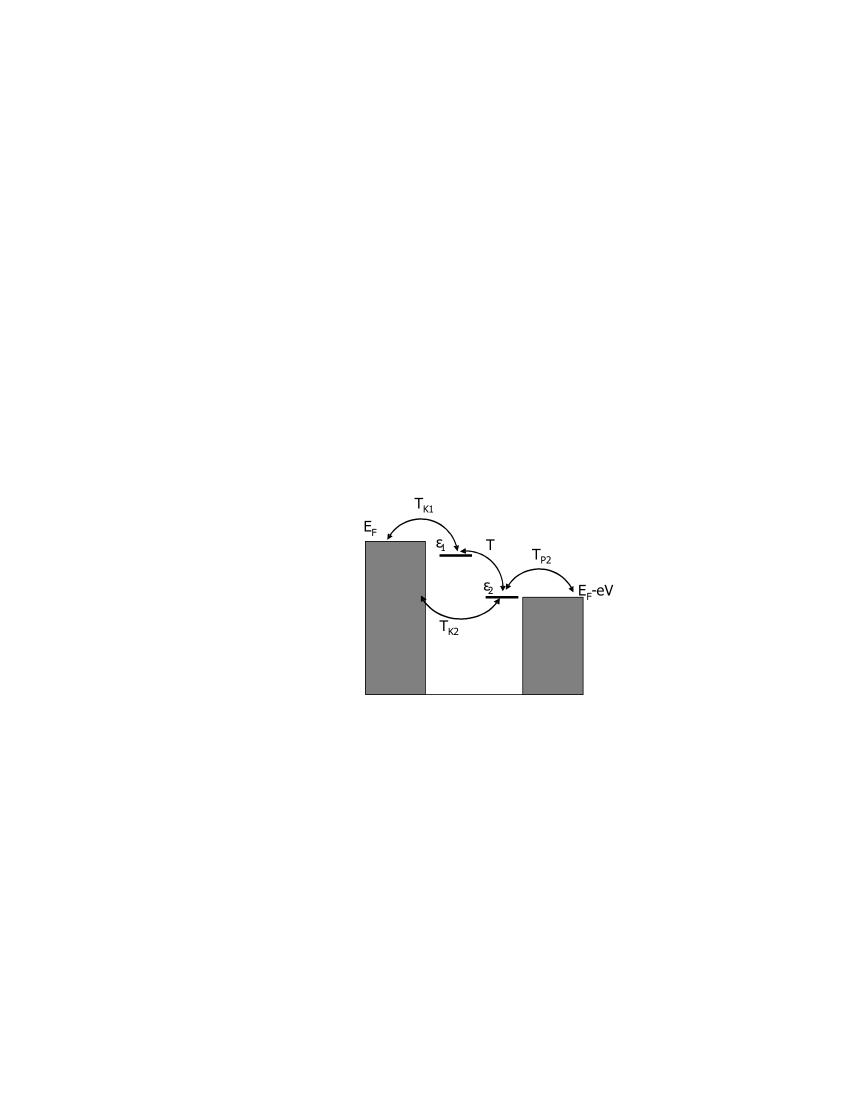
Figure 1: Schematic diagram of tunneling processes through states localized on impurity atom and on the STM tip apex.

Current noise correlation function is determined as:

$$(\hbar/e)^{2}\cdot S(t,t^{\prime})=<I_{L}(t)\cdot{I_{L}(t^{\prime})}>=$$

$$=\sum_{k,k^{{}^{\prime}},i,j}T_{k}^{2}<c_{k}^{+}(t^{\prime})a_{i}(t^{\prime})a_{j}^{+}(t)c_{k_{{}^{\prime}}}^{+}(t)>\$$ (2)

where

$$I_{L}(t)=\sum_{k}\dot{n}_{k}\cdot e=(\sum_{k}c_{k}^{+}(t^{\prime})a_{i}(t^{\prime})T_{ki}-h.c.)\cdot\frac{e}{\hbar}\$$ (3)

The current noise spectra is determined by Fourier transformation of $S(t,t^{\prime})$: $S(\omega)=\int S(\tau)d\tau\cdot e^{i\omega\tau}$.

We shall use Keldysh diagram technique in our study of low frequency tunneling current noise spectra Keldysh . Tunneling current noise spectra $S(\omega)$ can be expressed through Keldysh Green functions.

For the one localized state in tunneling contact one should put: $T=0$, $T_{k2}=0$, $\varepsilon_{2}=0$.

Expression for tunneling current noise spectra without Coulomb re-normalization of the tunneling vertexes can be found from diagrams shown on Fig. 2a and has the form:

$$( \hbar /e)^{2}\cdot S_{0}(\omega)=T_{k1}^{2}\cdot\sum_{k,k_{1}}(G_{kk_{1}}^{<}(\omega)\cdot G_{11}^{>}(\omega+\omega^{\prime})+$$ (4)

$$+ G_{11}^{<}(\omega)\cdot G_{kk_{1}}^{>}(\omega+\omega^{\prime}))+T_{k1}^{2}\cdot\sum_{k,k_{1}}(G_{k1}^{<}(\omega)\cdot$$

$$\cdot G_{k_{1}1}^{>}(\omega+\omega^{\prime})+G_{k_{1}1}^{<}(\omega)\cdot G_{k1}^{>}(\omega+\omega^{\prime}))\$$

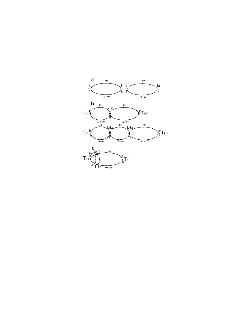
Figure 2: Lowest order diagrams contributing to tunneling current noise spectra for one localized state in tunneling contact. a) In the absence of Coulomb re-normalization of tunneling vertexes. b) In the presence of Coulomb re-normalization of tunneling vertexes - ladder diagrams. c) In the presence of Coulomb re-normalization of tunneling vertexes - parquet diagrams. Tunneling vertexes are marked by the dot. Coulomb potential is marked by the bold dot. Solid lines correspond to electron Green functions.

Green functions are evaluated from equations:

$$G_{kk_{1}}^{<} = G_{kk_{1}}^{0<}+G_{kk}^{0R}\sum_{k,k^{{}^{\prime}}}T_{k^{{}^{\prime}}}G_{k^{{}^{\prime}}k_{1}}^{<}+G_{kk}^{0<}\sum_{k,k^{{}^{\prime}}}T_{k^{{}^{\prime}}}G_{k^{{}^{\prime}}k_{1}}^{A}$$

$$G_{k1}^{<} = G_{kk}^{0R}T_{k1}G_{11}^{<}+G_{kk}^{0<}T_{k1}G_{11}^{A}$$ (5)

$$G_{11}^{<} = -2in(\omega)ImG_{11}^{R}(\omega)$$

Functions $G_{k_{1}k}^{>}$ and $G_{1k}^{>}$ can be found by substitution $n_{1}$ on $n_{1}-1$.

$$n_{1}(\omega)=\frac{\gamma_{k1}n_{k}^{o}(\omega)+\gamma_{p1}n_{p}^{o}(\omega)}{\gamma_{k1}+\gamma_{p1}}$$ (6)

are non-equilibrium localized state filling numbers.

$n_{k}^{o}(\omega)$ and $n_{p}^{o}(\omega)$- equilibrium filling numbers in the leads. In our model relaxation rates $\gamma_{ki}$, $\gamma_{pi}$ are determined by electron tunneling transitions from localized states to the leads $k$ and $p$ continuum states:

$$\sum_{p}T_{pi}^{2}ImG_{pp}^{0R}=\gamma_{pi};\sum_{k}T_{ki}^{2}ImG_{kk}^{0R}=\gamma_{ki}\$$ (7)

For tunneling current noise spectra without Coulomb re-normalization of tunneling vertexes after substitution the correspondent Green functions can be written as:

$$( \hbar/e)^{2}\cdot S_{0}(\omega)=\gamma_{k1}^{2}\cdot\int d\omega^{\prime}ImG_{11}^{R}(\omega^{\prime})\cdot$$ (8)

$$\cdot ImG_{11}^{R}(\omega+\omega^{\prime})\cdot(n_{1}(\omega+\omega^{\prime})-1)\cdot$$

$$\cdot (n_{1}(\omega^{\prime})-n_{k}(\omega^{\prime}))+n_{1}(\omega^{\prime})\cdot(n_{1}(\omega+\omega^{\prime})-$$

$$- n_{k}(\omega+\omega^{\prime})+\gamma_{k1}^{2}\cdot\int d\omega^{\prime}ImG_{11}^{R}(\omega^{\prime})\cdot$$

$$\cdot ImG_{11}^{R}(\omega+\omega^{\prime})\cdot(n_{k}(\omega+\omega^{\prime})-1)\cdot n_{1}(\omega^{\prime})-$$

$$- n_{1}(\omega^{\prime})\cdot(n_{1}(\omega+\omega^{\prime})-1)-n_{k}(\omega+\omega^{\prime})\cdot\ n_{k}(\omega^{\prime})+$$

$$+ n_{k}(\omega^{\prime})\cdot(n_{1}(\omega+\omega^{\prime})+\gamma_{k1}\cdot\int d\omega^{\prime}ImG_{11}^{R}(\omega+\omega^{\prime})\cdot$$

$$\cdot (n_{k}(\omega^{\prime}))\cdot(n_{1}(\omega+\omega^{\prime})-1)+ImG_{11}^{R}(\omega^{\prime})\cdot$$

$$\cdot (n_{1}(\omega^{\prime}))\cdot(n_{k}(\omega+\omega^{\prime})-1)=\widetilde{S}_{0}\$$

This expression gives us an opportunity to analyze tunneling current noise spectra for typical values of kinetic parameters of tunneling contact when localized charge is connected with the tip apex state $eV=\varepsilon_{1}$. Some low frequency spectra are shown on Fig. 3a.

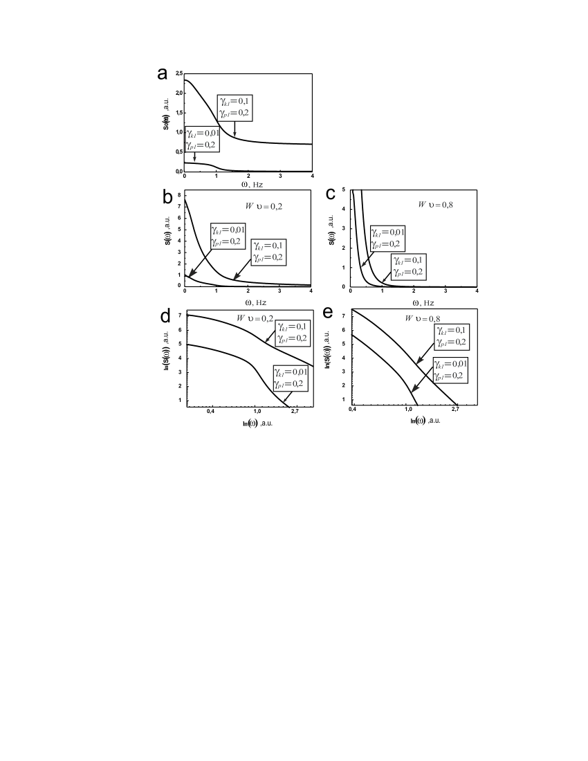
Figure 3: Typical low frequency tunneling current noise spectra for different values of dimensionless kinetic parameters for one localized state in tunneling contact ($eV=\varepsilon_{1}=1$). a) In the absence of Coulomb re-normalization of tunneling vertexes. b)-c) In the presence of Coulomb re-normalization of tunneling vertexes. d)-e) In the presence of Coulomb re-normalization of tunneling vertexes in double logarithmic scale.

It is clearly evident that when frequency aspire to zero tunneling current spectra aspire to constant value.

Now let us consider re-normalization of the tunneling amplitude and vertex corrections to the tunneling current noise spectra caused by Coulomb interaction between charged localized state and the electrons in tunneling contact leads. The result of re-normalization is shown on Fig. 2b and Fig. 2c. Re-normalization gives us two types of diagrams contributing to the final tunneling current noise spectra expression. Ladder diagrams is the most simple type of diagrams which gives logarithmic corrections to vertexes. Ladder diagrams give logarithmic divergency at the threshold voltage $eV=\varepsilon_{1}$ (Fig. 2b). But this is not the only relevant kind of graphs. We must consider one more type of graphs (parquet graphs) which gives logarithmically large contribution to tunneling spectra when $\omega\rightarrow 0$ and $eV=\varepsilon_{1}$ (Fig. 2c). In parquet graphs a new type of ”bubble” appears instead of ”dots” in ladder diagrams. In this situation one should retain in the n-th order of perturbation expansion the most divergent terms. For the first time this method was developed by Dyatlov et. al. Dyatlov . It was shown that for proper treatment of this problem one should write down integral equations for the so called parquet graphs, which are constructed by successive substitution the simple Coulomb vertex for the two types of bubbles in perturbation series. The integral equations can be solved with logarithmic accuracy, as it was done, for example, by Nozieres for edge singularities in X-ray absorption spectra in metals Nozieres . The expression for tunneling current noise spectra after Coulomb re-normalization can be written as:

$$( \hbar/e)^{2}\cdot S(\omega)=\widetilde{S}_{0}(\omega)+\widetilde{S}_{0}(\omega)\cdot$$ (9)

$$\cdot ((\frac{D^{2}}{(\omega+eV-\varepsilon_{1})^{2}+(\gamma_{k1}+\gamma_{p1})^{2}})^{W\nu}+$$

$$+ (\frac{D^{2}}{(-\omega+eV-\varepsilon_{1})^{2}+(\gamma_{k1}+\gamma_{p1})^{2}})^{W\nu})\$$

where D is the bandwidth for electrons in tunneling contact leads, , W-Coulomb potential, $\nu$- the equilibrium density of states in the tunneling contact leads. We consider that localized state is formed by STM tip apex, so we have to put $eV=\varepsilon_{1}$. Then we obtain final expression:

$$(\hbar/e)^{2}\cdot S(\omega)=\widetilde{S}_{0}(\omega)(1+(\frac{D^{2}}{\omega^{2}+(\gamma_{k1}+\gamma_{p1})^{2}})^{W\nu})\$$ (10)

Fig. 3b-3c demonstrate low frequency tunneling current noise spectra for typical values of dimensionless kinetic parameters. We can see that re-normalization of tunneling matrix element by switched ”on” and ”off” Coulomb potential of charged impurity lead to typical power law singularity in low frequency tunneling current noise spectra.

Some tunneling current noise spectra in double logarithmic scale for typical values of kinetic parameters are shown on Fig. 3d-3e. Low frequency tunneling current noise spectra in double logarithmic scale make it clear that power law exponent depends only on Coulomb potential of charged impurity and does not depend on tunneling contact parameters.

Now let’s describe interaction effects of two localized states in tunneling contact: surface localized state, formed by impurity atom, and localized STM tip apex state (Fig. 1). Expression which describes tunneling current noise spectra without Coulomb re-normalization can be calculated from graphs, shown in Fig. 4a. It consists of three parts.

$$\widetilde{S}_{0}(\omega)=\widetilde{S}_{01}(\omega)+\widetilde{S}_{02}(\omega)+\widetilde{S}_{03}(\omega)\$$ (11)

$\widetilde{S}_{01}(\omega)$ and $\widetilde{S}_{02}(\omega)$ are rather simple parts equal to tunneling current noise spectra without Coulomb re-normalization in the case of one localized state in tunneling contact Eq. (8). $\widetilde{S}_{03}(\omega)$ is not trivial, it exists only due to electron tunneling transitions from one lead to both localized states. Green functions shown on the graphs are found in Maslova . The contribution of $\widetilde{S}_{01}(\omega)$ is given by graphs with $i=j=1$ (Fig. 4a), $\widetilde{S}_{02}(\omega)$ is described by graph with $i=j=2$ (Fig. 4a), $\widetilde{S}_{03}(\omega)$ is given by diagrams with $i\neq j$ (Fig. 4a). The final expression for tunneling current noise spectra for two localized states in tunneling contact without Coulomb re-normalization of tunneling vertexes after substitution the correspondent Green functions can be written as:

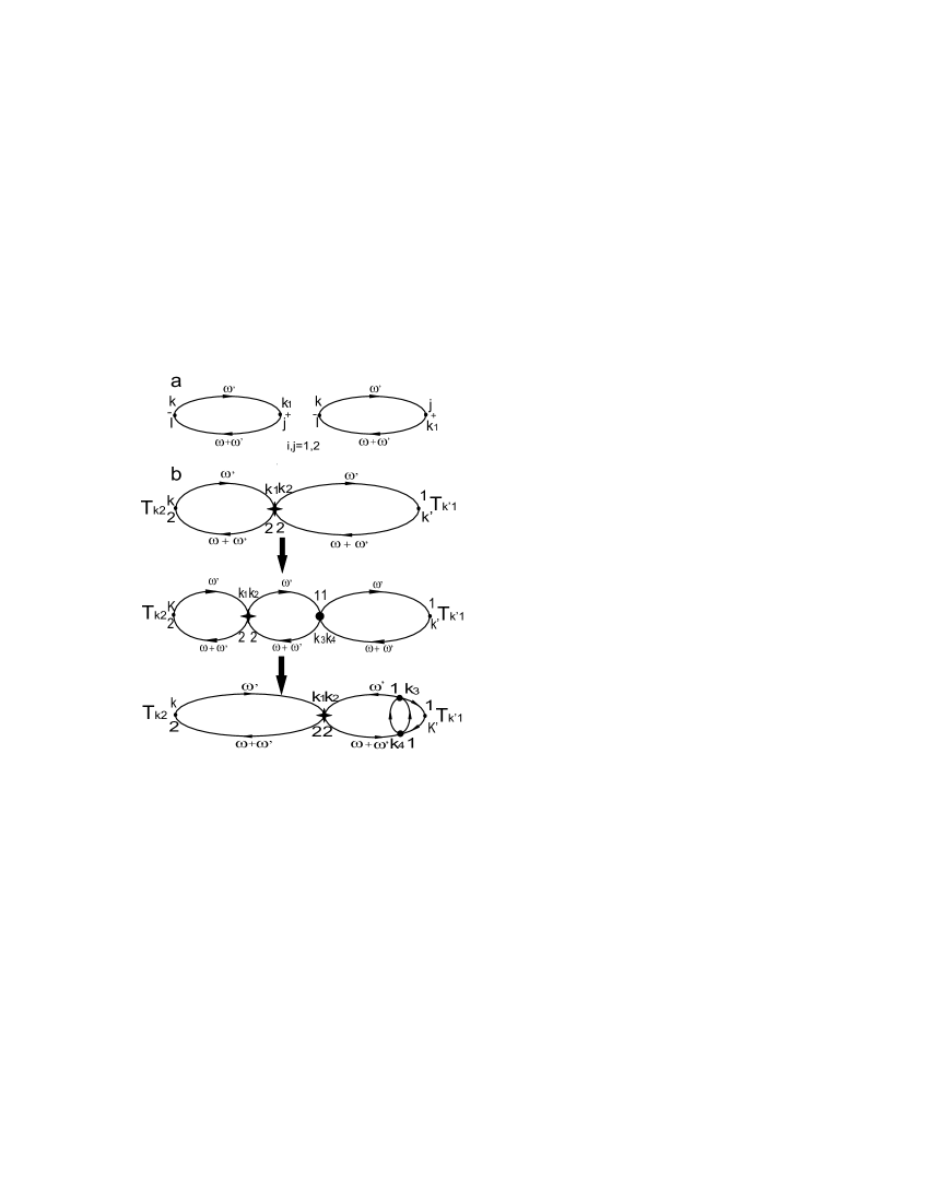
Figure 4: Lowest order diagrams contributing to tunneling current noise spectra for two localized states in tunneling contact. a) In the absence of Coulomb re-normalization of tunneling vertexes. b) In the presence of Coulomb re-normalization of tunneling vertexes. Tunneling vertexes are marked by the dot. Coulomb potential $W_{1}$ is marked by the bold dot. Coulomb potential $W_{2}$ is marked by the star. Solid lines correspond to electron Green functions.

$$( \hbar/e)^{2}\cdot S_{03}(\omega)=8\cdot\gamma_{k_{1}}\cdot\gamma_{k_{2}}\cdot\int d\omega^{\prime}ImG_{11}^{R}(\omega^{\prime})\cdot$$ (12)

$$\cdot ImG_{22}^{R}(\omega+\omega^{\prime})\cdot(n_{1}(\omega^{\prime})\cdot(n_{2}(\omega+\omega^{\prime})-1)+$$

$$+ n_{k}(\omega^{\prime})\cdot(n_{2}(\omega+\omega^{\prime})-1)+(n_{1}(\omega^{\prime})\cdot$$

$$\cdot (n_{k}(\omega+\omega^{\prime})-1)-n_{k}(\omega^{\prime})\cdot(n_{k}(\omega+\omega^{\prime})-1)+$$

$$+ 8\cdot\gamma_{k_{1}}\cdot\gamma_{k_{2}}\cdot\int d\omega^{\prime}ImG_{22}^{R}(\omega^{\prime})\cdot ImG_{11}^{R}(\omega+\omega^{\prime})\cdot$$

$$\cdot (n_{2}(\omega^{\prime})\cdot(n_{1}(\omega+\omega^{\prime})-1)+$$

$$+ n_{k}(\omega^{\prime})\cdot(n_{1}(\omega+\omega^{\prime})-1)+(n_{2}(\omega^{\prime})\cdot$$

$$\cdot (n_{k}(\omega+\omega^{\prime})-1)-n_{k}(\omega^{\prime})\cdot(n_{k}(\omega+\omega^{\prime})-1)\$$

Non-equilibrium filling numbers $n_{1}$ and $n_{2}$ are determined from Dyson equations for Keldysh functions $G_{ij}^{<}$, where $i,j=1,2$ in Maslova :

Green functions $G_{11}^{R},G_{22}^{R}$ have rather simple form and have been also derived in Maslova . We don’t take in account diagrams including Green functions $G_{12}^{<},G_{21}^{<}$. In our case of weak interaction between localized states $(T<\gamma_{k1},\gamma_{k2},\gamma_{p2})$ contribution to the noise spectra of such diagrams has additional small parameter in comparison with diagrams depicted on Fig.4a:

$$\frac{T\cdot\gamma_{k1}}{(\varepsilon_{1}-\varepsilon_{2})^{2}+(\gamma_{k1}+\gamma_{k2}+\gamma_{p2})^{2}}\sim T/\gamma$$ (13)

Some typical low frequency tunneling current noise spectra for different values of dimensionless kinetic parameters without Coulomb re normalization are shown on Fig. 5a. It is clearly evident that when frequency aspire to zero tunneling current spectra aspire to constant value for different dimensionless kinetic parameters. Now let us consider re-normalization of the tunneling amplitude and vertex corrections to the tunneling current spectra caused by Coulomb interaction between both localized states and tunneling contact leads. Re-normalization gives us two types of diagrams contributing to the final tunneling current noise spectra expression similar to types of graphs in the case of one localized state in tunneling contact. It is necessary to re-normalize each vertex individually and re-normalize both vertexes jointly. For each diagram re-normalized by Coulomb potential of localized state one have to take in to account the whole series of diagrams including Coulomb interaction with another localized state (Fig. 4b).

The final expression for tunneling current noise spectra after Coulomb re-normalization of tunneling vertexes can be written as:

$$( \hbar/e)^{2}\cdot S(\omega)=\widetilde{S}_{0}(\omega)+\widetilde{S}_{01}(\omega)\cdot$$

$$\cdot ((\frac{D^{2}}{(\omega+E_{1})^{2}+\Gamma_{2}^{2}})^{W_{1}\nu}+(\frac{D^{2}}{(\omega+E_{2})^{2}+\Gamma_{1}^{2}})^{W_{1}\nu})+$$

$$+ \widetilde{S}_{02}(\omega)\cdot((\frac{D^{2}}{(-\omega+E_{1})^{2}+\Gamma_{1}^{2}})^{W_{2}\nu}+$$

$$+ (\frac{D^{2}}{(-\omega+E_{2})^{2}+\Gamma_{2}^{2}})^{W_{2}\nu})+\widetilde{S}_{03}(\omega)\cdot$$

$$\cdot ((\frac{D^{2}}{(\omega+E_{1})^{2}+\Gamma_{2}^{2}})^{W_{1}\nu}+(\frac{D^{2}}{(\omega+E_{2})^{2}+\Gamma_{1}^{2}})^{W_{1}\nu})\cdot$$

$$\cdot ((\frac{D^{2}}{(-\omega+E_{1})^{2}+\Gamma_{1}^{2}})^{W_{2}\nu}+(\frac{D^{2}}{(-\omega+E_{2})^{2}+\Gamma_{2}^{2}})^{W_{2}\nu})$$

where,

$$E_{1} = eV-\frac{\varepsilon_{1}+\varepsilon_{2}}{2}+\frac{\sqrt{(\varepsilon_{1}-\varepsilon_{2})^{2}+4T^{2}}}{2}$$

$$E_{2} = eV-\frac{\varepsilon_{1}+\varepsilon_{2}}{2}-\frac{\sqrt{(\varepsilon_{1}-\varepsilon_{2})^{2}+4T^{2}}}{2}$$ (15)

$$\Gamma_{1} = \frac{(\varepsilon_{1}-\varepsilon_{2})(\gamma_{k2}+\gamma_{p2}-\gamma_{k1})}{2\sqrt{(\varepsilon_{1}-\varepsilon_{2})^{2}+4T^{2}}}+\frac{\gamma_{k2}+\gamma_{p2}-\gamma_{k1}}{2}$$

$$\Gamma_{2} = \frac{(\varepsilon_{1}-\varepsilon_{2})(\gamma_{k2}+\gamma_{p2}-\gamma_{k1})}{2\sqrt{(\varepsilon_{1}-\varepsilon_{2})^{2}+4T^{2}}}-\frac{\gamma_{k2}+\gamma_{p2}-\gamma_{k1}}{2}$$

When the applied bias voltage become close to $\varepsilon_{2}$ we obtain low frequency tunneling spectra. So we have to put $eV=\varepsilon_{1}=\varepsilon_{2}$. We obtain the expression:

$$( \hbar/e)^{2}\cdot S(\omega)=\widetilde{S}_{0}(\omega)+\widetilde{S}_{01}(\omega)\cdot((\frac{D^{2}}{\omega^{2}+\Gamma_{1}^{2}})^{W_{1}\nu}+$$

$$+ (\frac{D^{2}}{\omega^{2}+\Gamma_{1}^{2}})^{W_{1}\nu})+\widetilde{S}_{02}(\omega)\cdot((\frac{D^{2}}{\omega^{2}+\Gamma_{1}^{2}})^{W_{2}\nu}+$$

$$+ (\frac{D^{2}}{\omega^{2}+\Gamma_{1}^{2}})^{W_{2}\nu})+\widetilde{S}_{03}(\omega)\cdot((\frac{D^{2}}{\omega^{2}+\Gamma_{1}^{2}})^{W_{1}\nu}+$$

$$+ (\frac{D^{2}}{\omega^{2}+\Gamma_{1}^{2}})^{W_{1}\nu})\cdot((\frac{D^{2}}{\omega^{2}+\Gamma_{1}^{2}})^{W_{2}\nu}+(\frac{D^{2}}{\omega^{2}+\Gamma_{1}^{2}})^{W_{2}\nu})$$

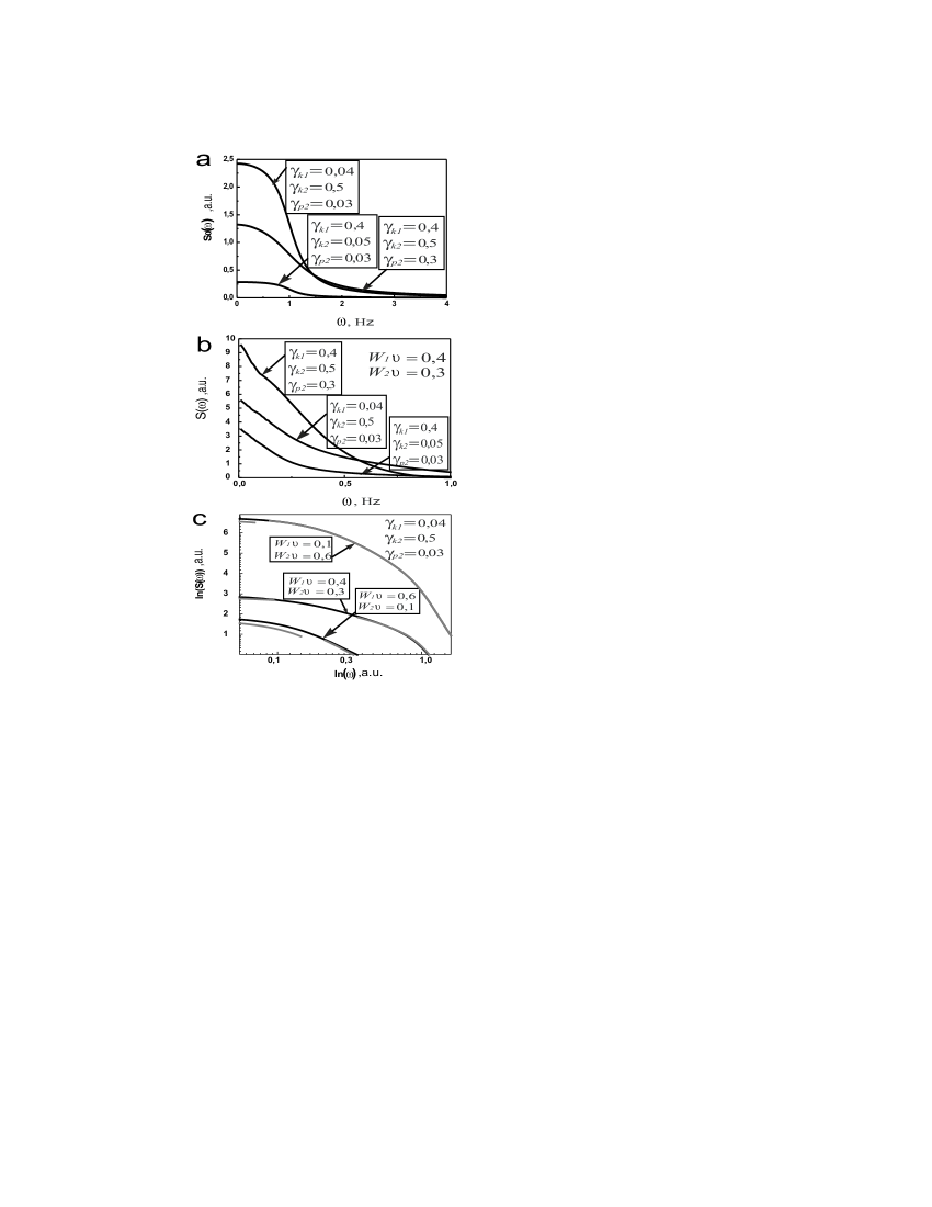
Figure 5: Typical low frequency tunneling current noise spectra for different values of dimensionless kinetic parameters for two localized states in tunneling contact ($eV=\varepsilon_{1}=\varepsilon_{2}=1$). a) In the absence of Coulomb re-normalization of tunneling vertexes. b) In the presence of Coulomb re-normalization of tunneling vertexes. c) In the presence of Coulomb re-normalization of tunneling vertexes in double logarithmic scale. Black lines correspond to tunneling current noise spectra in double logarithmic scale. Gray lines correspond to the terms which produce the most strong logarithmic singularity and approximate full spectra in the best way.

First of all we consider the situation when both localized states acquire positive charge. Fig. 5b demonstrate low frequency tunneling current noise spectra for typical values of dimensionless kinetic parameters. We can see that re-normalization of tunneling matrix element by switched ”on” and ”off” Coulomb potential of charged impurities lead to typical power law singularity in low frequency tunneling current noise spectra. Tunneling current noise spectra in double logarithmic scale demonstrate frequency regions where every part of final expression which include different power law exponent, approximate noise spectra in the best way (Fig. 5c). Let’s analyse tunneling current spectra shown on Fig. 5c. Contribution to tunneling current spectra at low (zero) frequency is always determined by the term which produces the most strong of logarithmic singularity, determined by the sum of localized states Coulomb potentials at any values of dimensionless tunneling rates of tunneling contact. In the case of $W_{1}>>W_{2}$ (Coulomb potential of charged impurity atom is larger than Coulomb potential of charged tip apex localized state) with frequency increasing the main contribution to tunneling current noise spectra is given by the term depending on Coulomb potential of localized state caused by impurity atom $(W_{1})$ at any dimensionless kinetic parameters of tunneling contact. If Coulomb potential of charged tip apex localized state is larger than Coulomb potential of charged impurity atom $(W_{2}>>W_{1})$ with frequency increasing the main contribution to tunneling current noise spectra is given by the term depending on Coulomb potential of tip apex localized state $(W_{2})$ at any dimensionless kinetic parameters of tunneling contact. When Coulomb potential of charged tip apex localized state is similar to Coulomb potential of charged impurity atom $(W_{1}\sim W_{2})$ with frequency increasing the main contribution to tunneling current noise spectra can be given both by the term depending on Coulomb potential of tip apex localized state $(W_{2})$ and by the item depending on Coulomb potential of localized state caused by impurity atom $(W_{1})$ at any dimensionless kinetic parameters of tunneling contact. In this case the replacement of dominating term can take place. Simple estimation gives an opportunity to determine the validity of obtained expressions. For typical typical parameters of tunneling junction model in the zero frequency region power spectrum of tunneling current corresponds to experimental results. Power spectrum on zero frequency has the form:

$$S(0)\approx(\gamma_{eff}\cdot e/\hbar)^{2}\cdot(D/\gamma_{eff1})^{\nu\cdot W}\cdot(1/\bigtriangleup\omega)\$$ (17)

For typical $\gamma_{eff}$, $\gamma_{eff1}$ $\approx 10^{-13}$, $D\approx 10$, $W\approx 0,5$ $S(0)\approx 10^{-18}A^{2}/Hz$ Oreshkin .

III Conclusion

The microscopic theoretical approach describing tunneling current noise spectra taking in account many-particle interaction was proposed. When electron tunnels to or from localized state the charge of localized state rapidly changes. This results in sudden switching on and off of additional Coulomb potential in tunneling junction area, and leads to typical power law dependence for low frequency tunneling current noise spectra. In the case of two interacting positively charged localized states the power law exponent at low frequency is determined by the sum of Coulomb potentials. It was shown that if one of the Coulomb potentials strongly exceeds the other one this potential determine tunneling current noise spectra at low frequency with increasing of frequency. If $W_{1}\sim W_{2}$, tunneling current noise spectra can be determined both by Coulomb potential $W_{1}$, and by Coulomb potential of charged tip apex state $W_{2}$, depending on dimensionless kinetic parameters of tunneling contact. When localized states acquire charges of opposite signs tunneling current noise spectra in the low frequency region are approximated by the term depending on maximum positive value of Coulomb potentials $W_{1}$, $W_{2}$, $W_{1}-W_{2}$ or $W_{2}-W_{1}$.

We are grateful to A.I. Oreshkin and S.V. Savinov for discussions and useful remarks.

This work was partially supported by RFBR grants 06-02-17076-a, 06-02-17179-a, 05-02-19806-MF and the Council of the President of the Russian Federation for Support of Young Scientists and Leading Scientific School NSh-4599.2006.2 and NSh-4464.2006.2.

References

- (1) A.I. Oreshkin, V.N. Mantsevich, N.S. Maslova et al., JETP Letters, 85, (2007), 46
- (2) Yu.M. Galperin, K.A. Chao, Phys. Rev. B, 55, (1995), 12126
- (3) L.S. Levitov, G.B. Lesovik, JETP Letters, 55, (1992), 534
- (4) B.L. Altshuler, L.S. Levitov, A. Yu. Yakovets, JETP Letters, 59, (1994), 821
- (5) R. Moller, A. Esslinger, B. Koslowski, Appl. Phys. Lett. 55, (1989), 2360
- (6) T. Tiedje et al. J. Vac. Sci. Technol. B, A6, (1988), 372
- (7) M. Lozano, M. Tringides, Europhys.Lett., 30, (1995), 537
- (8) L.V. Keldysh, Sov. Phys JETP, 20, (1964), 1018
- (9) P.I. Arseev, N.S. Maslova, V.I. Panov et al., JETP Letters, 76, (2002), 287
- (10) I.T. Dyatlov, V.V. Sudakov and K.A. Ter-Martirosian, JhETF, 5, (1957), 631
- (11) P. Nozieres, C.T. De Dominicis Phys.Rev., 178, (1969), 1097
- (12) P.I. Arseev, N.S. Maslova, V.I. Panov et al., JETP, 94, (2002), 191