A complete one-loop calculation of electroweak supersymmetric effects in -channel single top production at LHC
Abstract
We have computed the complete one-loop electroweak effects in the MSSM for single top (and single antitop) production in the -channel at hadron colliders, generalizing a previous analysis performed for the dominant final state and fully including QED effects. The results are quite similar for all processes. The overall Standard Model one-loop effect is small, of the few percent size. This is due to a compensation of weak and QED contributions that are of opposite sign. The genuine SUSY contribution is generally quite modest in the mSUGRA scenario. The experimental observables would therefore only practically depend, in this framework, on the CKM coupling.
pacs:
12.15.-y,12.15.Lk,13.75.Cs,14.80.LyI Introduction
The relevance of a precise measurement of single top production at hadron colliders was already stressed in several papers in the recent years Tait:1999cf . A well known peculiarity of the process is actually the fact that it offers the unique possibility of a direct measurement of the coupling , thus allowing severe tests of the conventionally assumed properties of the CKM matrix in the Minimal Standard Model; for a very accurate review of the topics we defer to Alwall:2006bx .
For the specific purpose of a ”precise” determination of ,
two independent requests must be met. The first one is that of a
correspondingly ”precise” experimental measurement of the process. For
the -channel case on which we shall concentrate in this paper the CMS
study Pumplin:2002vw concludes that, with fb-1 of
integrated luminosity, one could be able to reduce the (mostly systematic)
experimental uncertainty of the cross section below the ten percent
level (worse uncertainties are expected for the two other processes, the
-channel and the associated production, whose cross section is
definitely smaller than that of the -channel).
The second request is that of a similarly
accurate theoretical prediction of the observables of the process.
In this respect, one must make the precise statement that, in order to cope with the
goal of measuring at the few (five) percent level, a complete NLO
calculation is requested. In the SM this has been done for the QCD component
of the -channel, resulting in a relatively small (few percent)
effect Stelzer:1997ns .
The electroweak effects have been computed very recently at the
complete one loop level within the MSSM for the dominant component of the process
(to be defined in Section II) Beccaria:2006ir .
One conclusion was that the genuine SUSY effect, for a set on mSUGRA benchmark
points, was systematically modest, roughly at the one-two percent level.
The SM contribution was computed in a preliminary way, i.e. only including
the soft photon radiation to achieve cancellation of infrared singularities,
ignoring the potentially relevant hard photon contribution.
Actually, the main purpose of Beccaria:2006ir was that of investigating the possible
existence and size of genuine supersymmetric effects, that would be
essentially unaffected by the SM QED contribution.
In this approximate approach, the one-loop SM contribution turned out to be
sizable, of roughly ten percent on the total rate. This contribution should be
considered as a perfectly known term, to be included in the theoretical
expression of the rate and compared with the corresponding experimental
measurement to extract the precise value of the coupling .
In fact, from the negative (for what concerns supersymmetric searches) result
that the -channel rate is not sensitive to genuine mSUGRA MSSM effects,
adding the extra known feature that NLO QCD effects are small , of the order
of five percent, and well under
control QCDNLO QCDNLODecay Frixione:2005vw ,
one concludes that an extremely precise theoretical determination of
the process would be possible, provided that a rigorous electroweak
one-loop description were given. This requires two different steps:
first, an extension of the calculation of Beccaria:2006ir
to the seven remaining -channel processes since the final state is only the numerically dominant one.
Second, the additional calculation of the complete QED effect,
including properly hard photon radiation.
This is precisely the aim of this paper, whose goal will be that of offering
a clean theoretical expression to be used for a significant measurement of
.
Technically speaking, this paper is organized as follows. In Section
II the definition of the eight considered
processes will be given, and the main tasks that were fulfilled
to perform a complete one loop electroweak calculation will be indicated.
Since the problems to be solved were practically identical with
those already met in Beccaria:2006ir , our description will
be whenever possible quick and essential.
In Section III, we shall expose the new
calculation of the complete QED
effects.
In Section IV we briefly discuss the one loop SUSY QCD effects that we have recomputed
from scratch in the same scheme adopted for the electroweak corrections.
In Section V we shall define the considered observables
and show the results
of our calculation, particular emphasis being given to the value of the
total -channel rate.
A few conclusions will be drawn in the final Section VI.
II The -channel processes at one electroweak loop
The complete description of the -channel involves at
partonic level four sub-processes for single production: ,
, , ,
and the related four for the single production.
The starting point is the cross section for the process
with the complete set of one loop electroweak corrections (in the MSSM and SM).
The corrections to the (unpolarized) differential cross section of this process read:
| (1) |
where is the tree level contribution to the amplitude of the partonic process while describes the EW one loop contribution to the same amplitude. The Mandelstam variables are defined as:
| (2) | |||||
The analytical expression for is available in
literature (see for instance Beccaria:2006ir ).
has been generated with the help of FeynArts FeynArts , the algebraic reduction of the
one loop integrals is performed with the help of FormCalc FormCalc and
the scalar one loop integrals are numerically evaluated using LoopTools LoopTools .
We treat UV divergences using dimensional reduction while IR
singularities are parametrized giving a small mass to the photon. The masses of the light quarks
are used as regulators of the collinear singularities and are set to zero elsewhere.
UV divergences are cured renormalizing the parameters and the wavefunctions appearing in . In our case we have to renormalize the wavefunction of the
external quarks, the mass of the W boson, the electroweak mixing angle and the electric charge. We use the on shell scheme decribed in Ref. DennerHab .
This scheme uses the fine structure constant evaluated in the Thomson limit as input parameter. In order to avoid large logarithms arising from the runnning
of to the electroweak scale , we slightly modify this scheme using as input parameter the Fermi constant . We consistently change the definition
of the renormalization constant of the fine structure constant following the guidelines of Ref. WjetProd .
The unpolarized differential cross section for the process can be obtained from that of the process by crossing:
| (3) |
For the production the cross sections can be calculated using the identities
| (4) |
while the processes involving the second generation and quarks can be computed from the previous, simply replacing the masses of the external particles (and some masses in the loop corrections).
III QED effects
In order to obtain physically meanigful observables one has to include the differential cross section for
the process of -channel single top production associated with the
emission of a photon integrated over the whole photonic phase space.
So we have to consider the partonic processes
, , , ,
and the related four for the single production.
The unpolarized differential cross section of these processes has been obtained using two different procedures. In the first
approach the amplitude has been generated and squared using FeynArts and FormCalc while in the second one
the complete matrix element has been calculated with the help of FORM. The two methods are in mutual agreement.
The phase space integration of the aforementioned differential cross section is singular in the region in which the photon is soft
and in the region in which it is collinear to a massless quark.
According to KLN theorem KLN IR singularities and the
collinear singularities
related to the final state radiation cancel in sufficiently inclusive
observables while the collinear singularities related to initial state
radiation
have to be absorbed in the redefinition of the Parton Distribution
Functions (PDF). In order to
regularize these divergences
we use two different procedures: the Dipole Subtraction method and
the Phase Space Slicing method.
In the Subtraction approach one has to add and subtract
to the squared amplitude
an auxiliary function with the same asymptotic behaviour and
such that it can be analytically integrated
over the photon phase space. Among the different choices we
use the function quoted in Ref. Dipole .
In this Reference
explicit expression for the subtraction function and for its
analytical integration is obtained using
the so called Dipole Formalism DipoleQCD .
The idea behind the Phase Space Slicing approach is
to isolate the singular region of the phase
space introducing a cut off on the energy of the
photon () and on the
angle between the photon and
the massless quarks (). In the regular region the phase space integration can be done numerically while in the singular region
it can be performed analytically provided that the cutoffs are small enough. The form of the differential cross section in the
singular region is universal and its explicit expression in the soft (collinear) region can be
found in Ref. DennerHab (WjetProd ).
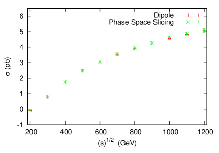
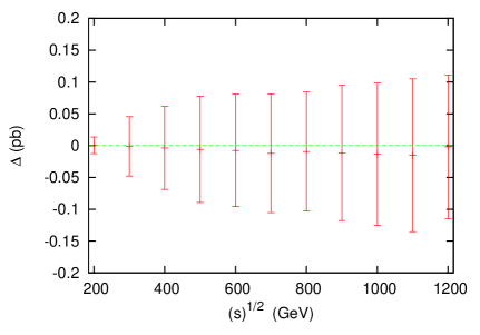
As can be inferred from Fig. 2 the two methods are in good numerical agreement.
IV One loop SUSY QCD corrections
The one loop SUSY QCD corrections to -channel single top production have been computed at LHC in Ref. Zhang:2006cx . We include these corrections re-computing them from scratch following the guidelines described in Sec. II. The only difference is that, following a standard procedure in SUSY QCD, we treat UV divergences using dimensional regularization. Moreover in this case we have to renormalize only the wavefunctions of the squarks since the other renormalization constant do not have corrections. These corrections are IR safe.
V Observable quantities
The differential hadronic cross section reads
| (5) | |||||
Where . The differential luminosity has been defined according to Ref. PinkBook while and . () are the (SUSY QCD) corrections to the differential cross section of the process .
As pointed out in Sec. III, initial state Collinear Singularities are not cancelled in the sum of virtual and real corrections and they are absorbed in the definition of the PDF. We use the factorization scheme at the scale . Concerning the choice of the parton distributions set, we follow WjetProd . The calculation of the full corrections to any hadronic observable must include QED effects in the DGLAP evolution equations. Such effects are taken into account in the MRST2004QED PDF Martin:2004dh which are NLO QCD. Since our computation is leading order QCD, we use the LO set CTEQ6L since the QED effects are known to be small Roth:2004ti .
V.1 Numerical Results
In this subsection we present our numerical results. We define as the invariant mass of the (anti)top quark and of the light quark in the final state. Also, we denote by the transverse momentum of the (anti)top quark. We consider as physical observables the transverse momentum distribution , the invariant mass distribution and two integrated observables derived from the previous: the integrated transverse momentum distribution, defined as the integral of from a minimum up to infinity:
| (6) |
and the cumulative invariant mass distribution , defined as the integral of the invariant mass distribution from the production threshold up to :
| (7) |
For each observable we present the plots for the LO and NLO curves and for the percentage effect of the NLO corrections to the observable . Apart from the Standard Model results, we analyzed several supersymmetric mSUGRA benchmark points: in the figures we present the numerical results for the two representative ATLAS DC2 mSUGRA benchmark points SU1 and SU6 DC2 ; in the other cases the results are similar. The SU1 and SU6 input parameters generate a moderately light supersymmetric scenarios, where the masses of the supersymmetric particles are below the : the two physical spectra are quite similar, characterized by relatively heavy squark sector ( for the lightest squark in SU1 and SU6 respectively), a light neutralino and a light chargino state. The typical masses for the supersymmetic Higgs are of order of . The main difference between the two points is the value of input parameter: for SU1 and for SU6.
V.1.1 SM Results
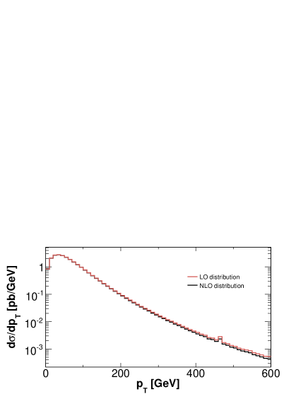
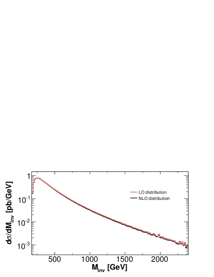
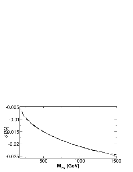
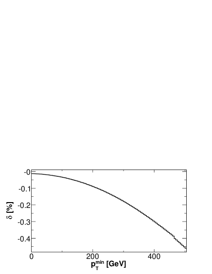
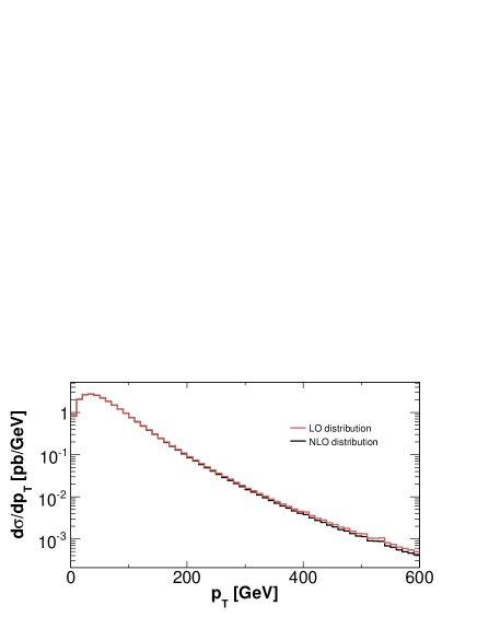
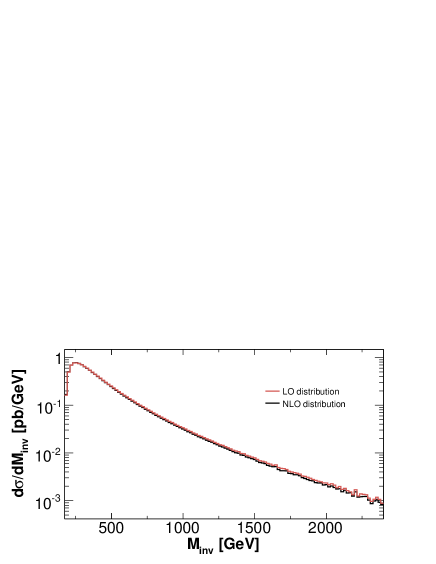
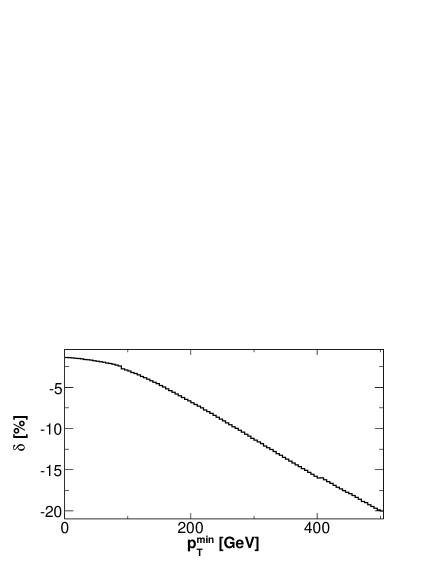
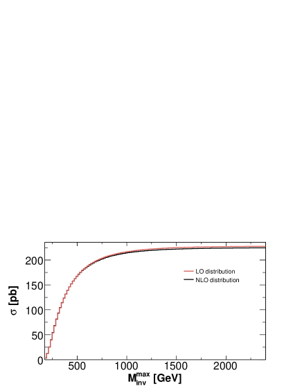
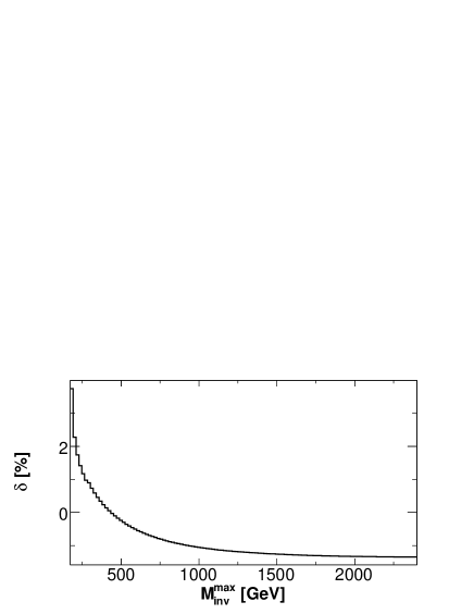
In the Standard Model framework the behaviour of the four observables is shown in Figures 3, 4, 5 and 6: the left panels report the LO and NLO curves, and the right panels show the relative percentage effect of the one loop electroweak corrections: as one can see the curves for the NLO and LO are almost overlapping, and the global NLO effect is rather small. This is particularly evident considering the plot for the cumulative invariant mass distribution, where the percentage effect saturate to the for .
V.1.2 MSSM Results
The following figures show the analogous
results for the transverse momentum distribution
, the invariant mass distribution , the integrated ditribution
and the cumulative invariant mass distribution
for the SU1
(Fig. 7, 8, 9, 10) and for
the SU6 (Fig. 11, 12, 13, 14) benchmark points.
In the MSSM cases the NLO is defined as the sum of the electroweak part
and of the SUSY QCD part; in each figure we show in the panel
(a) the behaviour of the observable at LO and NLO;
in (b) the global NLO effect (where ”global” means plus SUSY QCD);
in (c) and (d) the separate percentage contributions of
the and SUSY QCD parts respectively.
A first comment that can be drawn from the inspection of the plots is that the
-channel process is very weakly sensitive to the presence of the
supersymmetric particle in the loops. The difference with the Standard Model case, below
the percent level, is negligible for both the mSUGRA benchmark points, without
appreciable differences between the two sets.
The plots for percentage effect of the SUSY QCD corrections only
(the (d) panel in
Fig. 7, 8, 9, 10 for SU1 and
11, 12, 13, 14 for SU6)
show that the contribution of diagrams with virtual squark and gluinos
is systematically small, below the level, in agreement with Ref. Zhang:2006cx .
The same conclusion holds for the pure electroweak supersymmetric contribution,
being the effect due almost completely to the Standard Model part.
V.1.3 PDF uncertainties
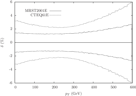
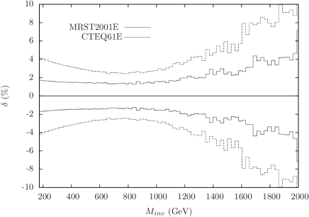
An important source of theoretical uncertainty is given by the contribution of the parametric errors associated with the parton densities. This could become particularly relevant for single top channels, due to the presence of an initial state quark, whose distribution function is strictly related to the gluon distribution. We have studied the impact of such uncertainties on the transverse momentum distribution and on the invariant mass distribution by using the PDF sets MRST2001E and CTEQ61E as in the LHAPDF package lhapdf . For each bin in the histograms the maximum and minimum values are calculated starting from the central value according to the formula , according to the prescription of Ref. pdfpage . The results are shown in Figure 15. The spread of the predictions obtained with the MRST set displays a relative deviation of about 2% or less, increasing on the large scale tails of the distributions (where the cross section is however very small), while the CTEQ set gives a larger uncertainty, of the order of 3-4%. This is due to different values of the tolerance parameter Tpdf , the latter being defined as the allowed maximum of the variation w.r.t. the parameters of the best PDFs fit. Conservatively, we can associate to our predictions an uncertainty due to the present knowledge of parton densities of about 3%. It is also worth noting that the uncertainties obtained according to such a procedure are of purely experimental origin only (i.e. as due to the systematic and statistical errors of the data used in the global fit), leaving aside other sources of uncertainty of theoretical origin.
VI Conclusions
We have computed in this paper the complete one-loop electroweak effect on various observables in the MSSM. The calculation has fully included QED effects. The overall result is that the one-loop effect is small, of a positive few percent in the total rate that we have considered as the first realistically measurable quantity. Technically speaking, this small number arises from a competition of negative weak contributions and positive QED terms. In the considered mSUGRA symmetry breaking scheme, the genuine SUSY effect in the considered benchmark points is systematically modest, at most of a one percent size. The values that we have obtained e.g. for the total rate should still be modified by the additional NLO QCD contribution. The latter is known, small and theoretically safe and could be easily added to our calculation. It will appear in a forthcoming paper that will provide an expression for the overall single top production at LHC, including the already existing calculations for the associated production (our paper and the QCD ones). We have also given an estimate of the parametric errors associated with the present knowledge of the parton densities. The distributions studied in this paper are affected by a few percent PDF uncertainty. It is worth saying that this uncertainty is expected to be lowered once the LHC data will become available. In conclusion, a precise measurement of the -channel rate appears as a perfect way to determine the value of the coupling, both within the SM and within the MSSM with mSUGRA symmetry breaking. We cannot exclude, though, that for different symmetry breaking mechanisms the genuine SUSY effect is more sizable. This question, that is beyond the purposes of this preliminary paper, remains open and, in our opinion, would deserve a special dedicated rigorous analysis.
Acknowledgements
We are gratefull to T. Hahn an S. Pozzorini for helpful discussions. E.M. is indebted with S. Dittmaier for
valuable suggestions on the Dipole Subtraction Formalism.
References
- (1) T. M. P. Tait, Phys. Rev. D 61, 034001 (2000) [arXiv:hep-ph/9909352].
- (2) J. Alwall et al., Eur. Phys. J. C 49, 791 (2007) [arXiv:hep-ph/0607115].
- (3) J. Pumplin, D. R. Stump, J. Huston, H. L. Lai, P. Nadolsky and W. K. Tung, “New generation of parton distributions with uncertainties from global QCD JHEP 0207, 012 (2002) [arXiv:hep-ph/0201195].
- (4) T. Stelzer, Z. Sullivan and S. Willenbrock, Phys. Rev. D 56, 5919 (1997) [arXiv:hep-ph/9705398].
- (5) M. Beccaria, G. Macorini, F. M. Renard and C. Verzegnassi, Phys. Rev. D 74, 013008 (2006) [arXiv:hep-ph/0605108].
- (6) B. W. Harris, E. Laenen, L. Phaf, Z. Sullivan and S. Weinzierl, Phys. Rev. D66 (2002) 054024 [arXiv:hep-ph/0207055]. Z. Sullivan, Phys. Rev. D70 (2004) 114012 [arXiv:hep-ph/0408049]. Z. Sullivan, Phys. Rev. D72 (2005) 094034 [arXiv:hep-ph/0510224]. S. Zhu, Phys. Lett. B524 (2002) 283–288 [Erratum: ibid B537 (2002) 351]. E.E. Boos, V.E. Bunichev, L.V. Dudko, V.I. Savrin and A.V. Sherstnev, Phys. Atom. Nucl. 69 (2006) 1317.
- (7) J. Campbell, R. K. Ellis and F. Tramontano, Phys. Rev. D70 (2004) 094012 [arXiv:hep-ph/0408158]. Q.-H. Cao and C. P. Yuan, Phys. Rev. D71 (2005) 054022 [arXiv:hep-ph/0408180]. Q.-H. Cao, R. Schwienhorst and C. P. Yuan, Phys. Rev. D71 (2005) 054023 [arXiv:hep-ph/0409040]. Q.-H. Cao, R. Schwienhorst, J. A. Benitez, R. Brock and C. P. Yuan, Phys. Rev. D72 (2005) 094027 [arXiv:hep-ph/0504230]. J. Campbell and F. Tramontano, Nucl. Phys. B726 (2005) 109–130 [arXiv:hep-ph/0506289].
- (8) S. Frixione, E. Laenen, P. Motylinski and B. R. Webber, JHEP 0603, 092 (2006) [arXiv:hep-ph/0512250]. S. Frixione, AIP Conf. Proc. 792, 685 (2005).
- (9) T. Hahn, Comput. Phys. Commun. 140, 418 (2001) [arXiv:hep-ph/0012260]; T. Hahn and C. Schappacher, Comput. Phys. Commun. 143, 54 (2002) [arXiv:hep-ph/0105349].
- (10) T. Hahn and M. Perez-Victoria, Comput. Phys. Commun. 118, 153 (1999) [arXiv:hep-ph/9807565].
- (11) T. Hahn, Acta Phys. Polon. B 30, 3469 (1999) [arXiv:hep-ph/9910227]; T. Hahn, Nucl. Phys. Proc. Suppl. 89, 231 (2000) [arXiv:hep-ph/0005029]; T. Hahn and M. Rauch, Nucl. Phys. Proc. Suppl. 157, 236 (2006) [arXiv:hep-ph/0601248].
- (12) A. Denner, Fortsch. Phys. 41, 307 (1993).
- (13) J. H. Kuhn, A. Kulesza, S. Pozzorini and M. Schulze, arXiv:0708.0476 [hep-ph]; W. Hollik, T. Kasprzik and B. A. Kniehl, arXiv:0707.2553 [hep-ph].
- (14) T. Kinoshita, J. Math. Phys. 3 (1962) 650; T. D. Lee and M. Nauenberg, Phys. Rev. 133, B1549 (1964).
- (15) S. Dittmaier, Nucl. Phys. B 565, 69 (2000) [arXiv:hep-ph/9904440].
- (16) S. Catani and M. H. Seymour, Phys. Lett. B 378, 287 (1996) [arXiv:hep-ph/9602277]; Nucl. Phys. B 485, 291 (1997) [Erratum-ibid. B 510, 503 (1998)] [arXiv:hep-ph/9605323]; S. Catani, S. Dittmaier, M. H. Seymour and Z. Trocsanyi, Nucl. Phys. B 627, 189 (2002) [arXiv:hep-ph/0201036].
- (17) J. J. Zhang, C. S. Li, Z. Li and L. L. Yang, Phys. Rev. D 75, 014020 (2007) [arXiv:hep-ph/0610087].
- (18) R. K. Ellis, W. J. Stirling and B. R. Webber, “QCD and collider physics,” Camb. Monogr. Part. Phys. Nucl. Phys. Cosmol. 8 (1996) 1.
- (19) A. D. Martin, R. G. Roberts, W. J. Stirling and R. S. Thorne, Eur. Phys. J. C 39, 155 (2005) [arXiv:hep-ph/0411040].
- (20) M. Roth and S. Weinzierl, Phys. Lett. B 590, 190 (2004) [arXiv:hep-ph/0403200].
- (21) ATLAS Data Challenge 2 DC2 points; http://paige.home.cern.ch/paige/fullsusy/romeindex.html.
- (22) http://hepforge.cedar.ac.uk/lhapdf/; M.R. Whalley, D. Bourilkov and R.C. Group, “The Les Houches Accord PDFs (LHAPDF) and Lhaglue”, arXiv:hep-ph/0508110 and references therein.
- (23) http://durpdg.dur.ac.uk/hepdata/pdf3.html.
-
(24)
A.D. Martin, R.G. Roberts, W.J. Stirling and R.S. Thorne, Eur. Phys. J.
C28, 455 (2003) [arXiv:hep-ph/0211080];
J. Pumplin, D.R. Stump, J. Houston, H.L. Lai, P. Nadolsky and W.K. Tung, JHEP 0207, 012 (2002) [arXiv:hep-ph/0201195].


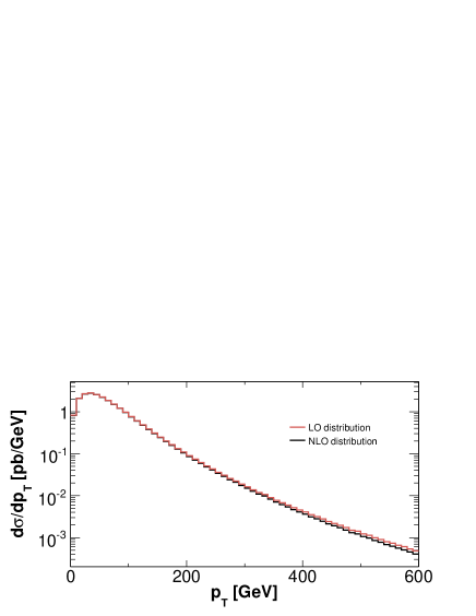

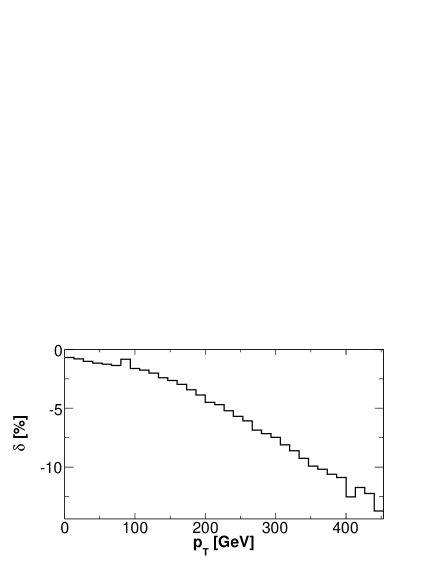
Right Panel: We plot the percentage contribution of the corrections to the transverse momentum distribution; that is .
No cuts are imposed. Computation in the Standard Model framework
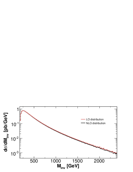

Right Panel: We plot the percentage contribution of the corrections to the invariant mass distribution; that is .
No cuts are imposed. Computation in the Standard Model framework
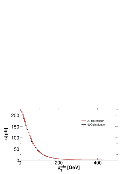

Right Panel: We plot the percentage contribution of the correections to the integrated transverse momentum distribution; that is . No cuts are imposed.Computation in the Standard Model framework


Right Panel: We plot the percentage contribution of the corrections to the cumulative invariant mass distribution; that is .
No cuts are imposed. Computation in the Standard Model framework
(a) (b)

(c) (d)

(b) We plot the percentage contribution of the plus SUSY QCD corrections to the transverse momentum distribution; that is .
(c) We plot the percentage contribution of the corrections to the transverse momentum distribution; that is .
(d) We plot the percentage contribution of the SUSY QCD corrections to the transverse momentum distribution; that is .
No cuts are imposed. Computation in the SU1 point
(a) (b)

(c) (d)

(b) We plot the percentage contribution of the plus SUSY QCD corrections to the invariant mass distribution; that is .
(c) We plot the percentage contribution of the corrections to the invariant mass distribution; that is .
(d) We plot the percentage contribution of the SUSY QCD corrections to the invariant mass distribution; that is .
No cuts are imposed. Computation in the SU1 point
(a) (b)


(c) (d)

(c) We plot the percentage contribution of the corrections to the integrated transverse momentum distribution; that is .
(d) We plot the percentage contribution of the SUSY QCD corrections to the integrated transverse momentum distribution; that is .
No cuts are imposed.Computation in the SU1 point
(a) (b)


(c) (d)


(c) We plot the percentage contribution of the corrections to the cumulative invariant mass distribution; that is .
(d) We plot the percentage contribution of the SUSY QCD corrections to the cumulative invariant mass distribution; that is .
No cuts are imposed. Computation in the SU1 point
(a) (b)

(c) (d)


(b) We plot the percentage contribution of the plus SUSY QCD corrections to the transverse momentum distribution; that is .
(c) We plot the percentage contribution of the corrections to the transverse momentum distribution; that is .
(d) We plot the percentage contribution of the SUSY QCD corrections to the transverse momentum distribution; that is .
No cuts are imposed. Computation in the SU6 point
(a) (b)

(c) (d)


(b) We plot the percentage contribution of the plus SUSY QCD corrections to the invariant mass distribution; that is .
(c) We plot the percentage contribution of the corrections to the invariant mass distribution; that is .
(d) We plot the percentage contribution of the SUSY QCD corrections to the invariant mass distribution; that is .
No cuts are imposed. Computation in the SU6 point
(a) (b)

(c) (d)


(c) We plot the percentage contribution of the corrections to the integrated transverse momentum distribution; that is .
(d) We plot the percentage contribution of the SUSY QCD corrections to the integrated transverse momentum distribution; that is .
No cuts are imposed.Computation in the SU6 point
(a) (b)

(c) (d)

(c) We plot the percentage contribution of the corrections to the cumulative invariant mass distribution; that is .
(d) We plot the percentage contribution of the SUSY QCD corrections to the cumulative invariant mass distribution; that is .
No cuts are imposed. Computation in the SU6 point