Exact stochastic simulation of dissipation and non-Markovian effects in open quantum systems

Abstract

The exact dynamics of a system coupled to an environment can be described by an integro-differential stochastic equation of its reduced density. The influence of the environment is incorporated through a mean-field which is both stochastic and non-local in time and where the standard two-times correlation functions of the environment appear naturally. Since no approximation is made, the presented theory incorporates exactly dissipative and non-Markovian effects. Applications to the spin-boson model coupled to a heat-bath with various coupling regimes and temperature show that the presented stochastic theory can be a valuable tool to simulate exactly the dynamics of open quantum systems. Links with stochastic Schroedinger equation method and possible extensions to ”imaginary time” propagation are discussed.

I Introduction

Numerous concepts in our understanding of quantum mechanics have emerged from the understanding and description of a system coupled to an environment: measurement, decoherence, appearance of classical world, irreversible process and dissipation… All these phenomena which are often encompassed in the ”theory of open quantum systems”, bridge different fields of physics and chemistry Weiss (1999); Joos et al. (2003); Breuer and Petruccione (2002). During the past decade, important advances have been made in the approximate and exact description of system embedded in an environment using stochastic methods. Recently the description of open quantum systems by Stochastic Schroedinger Equation (SSE) has received much attention Plenio and Knight (1998); Breuer and Petruccione (2002); Stockburger and Grabert (2002). Nowadays, Monte-Carlo wave-function techniques are extensively used to treat master equations in the weak coupling and/or Markovian limitDalibard et al. (1992); Dum et al. (1992); Gisin and Percival (1992); Carmichael (1993); Castin and Mo/lmer (1996); Rigo and Gisin (1996); Plenio and Knight (1998); Gardiner and Zoller (2000); Breuer and Petruccione (2002).

Large theoretical efforts are actually devoted to the introduction of non-Markovian effects. Among the most recent approaches, one could mention either deterministic approaches like Projection Operator techniques Breuer et al. (1999, 2001) or stochastic methods like Quantum State Diffusion (QSD) Diósi and Strunz (1996); Diósi et al. (1998); Strunz et al. (1999); Strunz (2005) where non-Markovian effects are accounted for through non-local memory kernels and state vectors evolve according to integro-differential stochastic equations. In some cases, these methods are shown to be exact Stockburger and Grabert (2002); Shao (2004).

Recently, alternative exact methodsBreuer (2004a); Lacroix (2005) have been developed to treat the system+environment problem that avoid evaluation of non-local memory kernel although non-Markovian effects are accounted for exactly. However, up to now, only few applications of these exact techniques exist Breuer et al. (2004); Breuer (2004b, a); Lacroix (2005); Zhou et al. (2005); Breuer and Petruccione (2007). In all cases, accurate description of the short time dynamics is obtained but long time evolution can hardly be described due to the large increase of statistical errors with time. Although, the possibility to simulate exactly the dissipative dynamics of open quantum systems is already an important step, the challenge to describe long-time evolution is highly desirable to make the techniques more powerful and versatile.

II Exact stochastic equation for the reduced system density

II.1 Introduction

In the present work, starting from the exact stochastic formulation of ref. Lacroix (2005) and projecting out the effect of the environment, an equation of motion for the reduced system dynamics is obtained where the environment effect is incorporated through a stochastic mean-field which turns out to be non-local in time. Advantages of the new stochastic theory for the description of long-time evolution of open quantum systems are underlined. We consider here a system (S) + environment (E) described by a Hamiltonian

$$H=h_{S}+h_{E}+h_{I},$$ (1)

where $h_{S}$ and $h_{E}$ denote the system and environment Hamiltonians respectively while $h_{I}$ is responsible for the coupling. Here we assume that the interaction writes

$$h_{I}=\mathbf{Q}\otimes\mathbf{B},$$ (2)

where $\mathbf{Q}\equiv f(\{Q_{i}\}_{i=1,n_{S}})$ and $\mathbf{B}\equiv g(\{B_{i}\}_{i=1,n_{B}})$ correspond to functions of two sets of operators of the system and environment, respectively. In particular, this definition includes non-linear couplings. For the sake of simplicity, we assume an initial separable density $D(t_{0})=\rho_{S}(t_{0})\otimes\rho_{B}(t_{0})$. As will be discussed below this assumption could be relaxed. The exact evolution of the system is described by the Liouville von-Neumann equation $i\hbar\dot{D}=\left[H,D\right].$ Due to the coupling, the simple separable structure of the initial condition is not preserved in time. It has however been realized recently in several works using either SSE or path integral techniques that the exact density of the total system $D(t)$ could be obtained as an average over simple separable densities, i.e. $D(t)=\overline{\rho_{S}(t)\otimes\rho_{B}(t)}$. In its simplest version, the stochastic process takes the form Lacroix (2005)

$$\left\{\begin{array}[]{lll}d\rho_{S}&=&\frac{dt}{i\hbar}[h_{S},\rho_{S}]+d\xi_{S}\mathbf{Q}\rho_{S}+d\lambda_{S}\rho_{S}\mathbf{Q}\\ \\ d\rho_{E}&=&\frac{dt}{i\hbar}[h_{E},\rho_{E}]+d\xi_{E}\mathbf{B}\rho_{E}+d\lambda_{E}\rho_{E}\mathbf{B}\end{array}\right.$$ (6)

where the Ito convention for stochastic calculations is usedGardiner (1985). $d\xi_{S/E}$ and $d\lambda_{S/E}$ denote Markovian Gaussian stochastic variables with zero means and variances

$$\overline{d\xi_{S}d\xi_{E}} = \frac{dt}{i\hbar},~{}~{}~{}~{}\overline{d\lambda_{S}d\lambda_{E}}=-\frac{dt}{i\hbar},$$ (7)

$$\overline{d\xi_{S}d\lambda_{E}} = \overline{d\lambda_{S}d\xi_{E}}=0.$$ (8)

The average over stochastic paths described by Eqs. (6) match the exact evolution. Indeed, assuming that at time $t$ the total density writes $D(t)=\rho_{S}(t)\otimes\rho_{B}(t)$, the average evolution over a small time step $dt$ is given by

$$\overline{dD}=\overline{d\rho_{S}\otimes\rho_{E}}+\overline{\rho_{S}\otimes d\rho_{E}}+\overline{d\rho_{S}\otimes d\rho_{E}}.$$ (9)

Using statistical properties of stochastic variables (Eqs. (7-8)), we obtain

$$\overline{d\rho_{S}\otimes\rho_{E}}+\overline{\rho_{S}\otimes d\rho_{E}} = \frac{dt}{i\hbar}[h_{S}+h_{E},\rho_{S}\otimes\rho_{E}],$$ (10)

$$\overline{d\rho_{S}\otimes d\rho_{E}} = \frac{dt}{i\hbar}[\mathbf{Q}\otimes\mathbf{B},\rho_{S}\otimes\rho_{E}].$$ (11)

Therefore, the last term simulates the interaction Hamiltonian exactly and the average evolution of the total density over a time step $dt$ reads

$$\overline{dD}=\frac{dt}{i\hbar}[H,D],$$ (12)

which is nothing but the exact evolution. Here, the exactness of the method is proved assuming that the density $D(t)$ is a single separable density. In practice, the total density at time $t$ is already an average over separable densities obtained along each stochastic path, i.e. $\overline{D(t)}=\overline{\rho_{S}(t)\otimes\rho_{E}(t)}$. Since Eq. (12) is valid for any density written as $\rho_{S}(t)\otimes\rho_{E}(t)$, by summing individual contributions, we deduce that the evolution of the total density obtained by averaging over different paths is given by $i\hbar d\overline{D}=dt[H,\overline{D(t)}]$ which is valid at any time and corresponds to the exact system+environment dynamics.

II.2 Stochastic mean-field dynamics

Here, a slightly modified version of the stochastic process is used. It incorporates part of the system/environment coupling using a ”mean-field” approximation in the deterministic evolution. Following ref. Lacroix (2005), we consider the coupled stochastic evolutions, called hereafter ”Stochastic Mean-Field” (SMF) :

$$\left\{\begin{array}[]{lll}d\rho_{S}&=&\frac{dt}{i\hbar}[h_{S}+\langle\mathbf{B}(t)\rangle_{E}\mathbf{Q},\rho_{S}]+d\xi_{S}(\mathbf{Q}-\langle\mathbf{Q}(t)\rangle_{S})\rho_{S}+d\lambda_{S}\rho_{S}(\mathbf{Q}-\langle\mathbf{Q}(t)\rangle_{S})\\ \\ d\rho_{E}&=&\frac{dt}{i\hbar}[h_{E}+\langle\mathbf{Q}(t)\rangle_{S}\mathbf{B},\rho_{E}]+d\xi_{E}(\mathbf{B}-\langle\mathbf{B}(t)\rangle_{E})\rho_{E}+d\lambda_{E}\rho_{E}(\mathbf{B}-\langle\mathbf{B}(t)\rangle_{E})\end{array}\right.,$$ (16)

where

$$\langle\mathbf{Q}(t)\rangle_{S}\equiv{\rm Tr}(\mathbf{Q}\rho_{S}(t)),~{}~{}~{}~{}\langle\mathbf{B}(t)\rangle_{E}\equiv{\rm Tr}(\mathbf{B}\rho_{E}(t)).$$ (17)

The SMF version also provides an exact reformulation of the system+environment problem. Indeed, the two terms in Eqs. (10-11) now read

$$\overline{d\rho_{S}\otimes\rho_{E}}+\overline{\rho_{S}\otimes d\rho_{E}} = \frac{dt}{i\hbar}[h_{S}+\langle\mathbf{B}(t)\rangle_{E}\mathbf{Q},\rho_{S}\otimes\rho_{E}]+\frac{dt}{i\hbar}[h_{E}+\langle\mathbf{Q}(t)\rangle_{S}\mathbf{B},\rho_{S}\otimes\rho_{E}]$$

$$\overline{d\rho_{S}\otimes d\rho_{E}} = \frac{dt}{i\hbar}[(\mathbf{Q}-\langle\mathbf{Q}(t)\rangle_{S})\otimes(\mathbf{B}-\langle\mathbf{B}(t)\rangle_{E}),\rho_{S}\otimes\rho_{E}].$$

and properly recombine to recover equation (12).

II.2.1 Properties of the SFM theory

Eqs. (16) have several advantages compared to the simple version (Eqs. (6)). First, this stochastic process automatically insures ${\rm Tr}(\rho_{E})={\rm Tr}(\rho_{S})=1$ along the stochastic path. In addition, the inclusion of a ”mean-field” term in the deterministic part will always reduce the statistical dispersion compared to the simple stochastic process given by Eqs. (6). This reduction could be significant if quantum fluctuations of the coupling operators $\mathbf{Q}$ and $\mathbf{B}$ remain small along each path Lacroix (2005, 2007). Indeed, at any time, a measure of the statistical fluctuations is given by

$$\lambda_{stat} = \overline{{\rm Tr}\Big{\{}\left(D^{\dagger}(t)-\overline{D^{\dagger}(t)}\right)\left(D(t)-\overline{D(t)}\right)\Big{\}}}$$ (18)

$$= \overline{{\rm Tr}\Big{\{}D^{\dagger}D(t)\Big{\}}}-{\rm Tr}\Big{\{}\overline{D(t)}^{2}\Big{\}}.$$

Starting from the total density associated to a pure state, the evolution of $\lambda_{stat}$ over a small time step is directly connected to the average quantum fluctuations of $\mathbf{Q}$ and $\mathbf{B}$, i.e.

$$d\lambda_{stat} = \frac{2dt}{\hbar}\Big{\{}\overline{(\langle\mathbf{Q}^{2}\rangle_{S}-\overline{\langle\mathbf{Q}\rangle}^{2}_{S})}+\overline{(\langle\mathbf{B}^{2}\rangle_{S}-\overline{\langle\mathbf{B}\rangle}^{2}_{S})}\Big{\}},$$ (19)

where, we have assumed implicitly that all second moments except those given in equations (7-8) cancel out. For comparison, the growth of statistical fluctuations associated to the stochastic process without mean-field (Eqs. (6)) reads

$$d\lambda_{stat} = \frac{2dt}{\hbar}\Big{\{}\overline{\left\langle\mathbf{Q}^{2}\right\rangle_{S}}+\overline{\left\langle\mathbf{B}^{2}\right\rangle_{E}}\Big{\}}.$$ (20)

Eq. (19) illustrates that the number of trajectories required to simulate the system dynamics will depend on the importance of quantum fluctuations of coupling operators along each path. In addition, a comparison between Eqs. (19) and (20) illustrates that the introduction of mean-field will always improve the numerical accuracy.

II.3 Reduced system evolution

In Eq. (16), the influence of the environment on the system only enters through $\langle\mathbf{B}(t)\rangle_{E}$. One expects in general to simplify the treatment by directly considering this observable evolution instead of the complete $\rho_{E}$ evolution. To express $\langle\mathbf{B}(t)\rangle_{E}$, we introduce the environment evolution operator

$$U_{E}(t,t^{\prime})\equiv\exp\left(\frac{1}{i\hbar}h_{E}(t-t^{\prime})\right).$$ (21)

Defining the new set of stochastic variables $dv_{E}$ and $du_{E}$ through $d\xi_{E}=dv_{E}-idu_{E}$ and $d\lambda_{E}=dv_{E}+idu_{E}$, the evolution of $\rho_{E}(t)$ can be integrated as

$$\rho_{E}(t) = U_{E}(t,t_{0})\rho_{E}(t_{0})U^{\dagger}_{E}(t,t_{0})+\int_{0}^{t}\frac{ds}{i\hbar}\langle\mathbf{Q}(s)\rangle_{S}~{}~{}U_{E}(t,s)[\mathbf{B},\rho_{E}(s)]U^{\dagger}_{E}(t,s)$$ (22)

$$+ \int_{0}^{t}dv_{E}(s)~{}~{}U_{E}(t,s)\{\mathbf{B}-\langle\mathbf{B}(s)\rangle_{E},\rho_{E}(s)\}_{+}U^{\dagger}_{E}(t,s)-i\int_{0}^{t}du_{E}(s)~{}~{}U_{E}(t,s)[\mathbf{B}-\langle\mathbf{B}(s)\rangle_{E},\rho_{E}(s)]U^{\dagger}_{E}(t,s).$$

Introducing also the new variables $du_{S}$ and $dv_{S}$ defined as $d\xi_{S}=du_{S}-idv_{S}$ and $d\lambda_{S}=du_{S}+idv_{S}$, the stochastic equation on the reduced density reads

$$d\rho_{S}=\frac{dt}{i\hbar}\left[{\cal H}_{S}(t),\rho_{S}\right]+du_{S}\{\mathbf{Q}-\langle\mathbf{Q}(t)\rangle_{S},\rho_{S}\}_{+}-idv_{S}[\mathbf{Q}-\langle\mathbf{Q}(t)\rangle_{S},\rho_{S}]$$ (23)

with ${\cal H}_{S}(t)\equiv h_{S}+\left\langle\mathbf{B}(t)\right\rangle_{E}\mathbf{Q}$ and where the source term $\left\langle\mathbf{B}(t)\right\rangle_{E}$ takes the exact form

$$\left\langle\mathbf{B}(t)\right\rangle_{E} = {\rm Tr}(\mathbf{B}^{I}(t-t_{0})\rho_{E}(t_{0}))-\frac{1}{\hbar}\int^{t}_{0}D(t,s)\left\langle\mathbf{Q}(s)\right\rangle_{S}ds-\int^{t}_{0}D(t,s)du_{E}(s)+\int^{t}_{0}D_{1}(t,s)dv_{E}(s).$$ (24)

Here, $\mathbf{B}^{I}(t-s)\equiv U^{\dagger}_{E}(t,s)\mathbf{B}U_{E}(t,s)$ while $D$ and $D_{1}$ are defined by:

$$D(t,s) \equiv i\langle[\mathbf{B},\mathbf{B}^{I}(t-s)]\rangle_{E},$$ (25)

$$D_{1}(t,s) \equiv \langle\{\mathbf{B}-\langle\mathbf{B}(s)\rangle_{E},\mathbf{B}^{I}(t-s)\}_{+}\rangle_{E},$$ (26)

where the environment expectation values are taken at time $s$, i.e. $\langle\cdots\rangle_{S}\equiv{\rm Tr}(\cdots\rho_{E}(s))$. The two coupled equations, Eqs. (23-24) provide an exact reformulation of the system evolution if $du_{S/E}$ and $dv_{S/E}$ verify

$$\begin{array}[]{ccc}\overline{du_{S}du_{E}}&=&\overline{dv_{S}dv_{E}}=\frac{dt}{2\hbar},\\ \overline{du_{S}dv_{E}}&=&\overline{dv_{S}du_{E}}=0.\end{array}$$ (29)

In the following, we simply assume that the first term in Eq. (24) cancels out. Substituting Eq. (24) into Eq. (23), we finally obtain an integro-differential stochastic equation for the exact system evolution where the environment effect has been incorporated through the two memory functions (25-26). The interesting aspect of replacing Eq.(16) by Eqs. (23-24) is that, in many physical situations, one can generally take advantage of specific commutation/anti-commutation properties of $\mathbf{B}$ as well as flexibility in the noise to obtain an explicit form of the memory functions.

III Application to system coupled to a heat-bath

The method is illustrated for systems coupled to an environment of harmonic oscillators initially at thermal equilibrium and it shows that the present stochastic theory can be a valuable tool to simulate exactly open quantum systems. We take

$$h_{E}=\sum_{n}\left(\frac{p^{2}_{n}}{2m_{n}}+\frac{1}{2}m_{n}\omega^{2}_{n}x^{2}_{n}\right)$$ (30)

and $\mathbf{B}\equiv-\sum_{n}\kappa_{n}x_{n}$ Breuer and Petruccione (2002). The statistical properties of stochastic variables $du_{S/E}$ and $dv_{S/E}$ specified above do not uniquely define the Wiener process. A simple prescription is to further assume

$$\left\{\begin{array}[]{lll}\overline{du_{S}du_{S}}&=&\overline{du_{E}du_{E}}=\overline{dv_{S}dv_{S}}=\overline{dv_{E}dv_{E}}=0,\\ \overline{du_{S}dv_{S}}&=&\overline{du_{E}dv_{E}}=0.\end{array}\right.$$ (33)

There are several advantages to this choice. First, stochastic calculus are greatly simplified. For instance, using standard techniques for system coupled to heat-bath Feynman and Vernon (1963); Caldeira and Leggett (1983) and Ito stochastic rules, shows that $D$ and $D_{1}$ depend only on the time difference $\tau=(t-s)$ and identify with the standard correlation functions Breuer and Petruccione (2002) (see appendix A):

$$D(\tau) = 2\hbar\int^{+\infty}_{0}d\omega J(\omega)\sin(\omega\tau),$$ (34)

$$D_{1}(\tau) = 2\hbar\int^{+\infty}_{0}d\omega J(\omega)\coth({\hbar\omega/2k_{B}T})\cos(\omega\tau),$$ (35)

where

$$J(\omega) \equiv \sum_{n}\frac{\kappa^{2}_{n}}{2m_{n}\omega_{n}}\delta(\omega-\omega_{n}),$$ (36)

denotes the spectral density. No approximation are made to obtain above equations, therefore the average over different stochastic paths match the exact evolution of the system, including all non-Markovian effects.

III.1 Equivalent Stochastic Schroedinger Equation formulation

Several works, based on the influence functional method Stockburger and Grabert (2002); Shao (2004); Yan et al. (2004) have led to similar stochastic equations for the reduced density. For instance, authors of ref. Shao (2004); Yan et al. (2004) use an evolution of $\left\langle\mathbf{B}(t)\right\rangle_{E}$ where the second term in Eq. (24) is absent. As demonstrated below, this term is of crucial importance for applications. In ref. Stockburger and Grabert (2002) and in refs. Breuer et al. (2004); Breuer (2004b); Lacroix (2005) a stochastic formulation of the exact system+environment is given in terms of the Stochastic Schroedinger Equation (SSE) technique. Thanks to the additional stochastic rules (33), Eq. (23) has also its SSE counterpart, where system densities are replaced by $\rho_{S}=\left|\phi_{1}\right\rangle\left\langle\phi_{2}\right|$ and wave functions evolve according to

$$\left\{\begin{array}[]{ccc}d\left|\phi_{1}\right\rangle&=&\{\frac{dt}{i\hbar}{\cal H}_{S}(t)+d\xi_{S}(\mathbf{Q}-\langle\mathbf{Q}(t)\rangle_{S})\}\left|\phi_{1}\right\rangle\\ \\ d\left\langle\phi_{2}\right|&=&\left\langle\phi_{2}\right|\{-\frac{dt}{i\hbar}{\cal H}_{S}(t)+d\lambda_{S}(\mathbf{Q}-\langle\mathbf{Q}(t)\rangle_{S})\}\end{array}\right..$$ (40)

where the bath effect is again incorporated through the mean-field kernel.

III.2 Application to the spin-boson model

We illustrate the proposed technique to the spin-boson model. This model can be regarded as one of the simplest quantum open system coupled to a heat bath Leggett et al. (1987) which could not be integrated exactly. In addition, it has been often used as a benchmark for theories of open quantum systems Leggett et al. (1987); Egger and Mak (1994); Diósi et al. (1998); Weiss (1999); Breuer et al. (2001); Stockburger and Grabert (2002); Shao (2004). The system and coupling Hamiltonians are respectively chosen as

$$h_{S}=\hbar\omega_{0}\sigma_{x}+\hbar\varepsilon\sigma_{z},~{}~{}~{}~{}h_{I}=\sigma_{x}\otimes\mathbf{B},$$

where the $\{\sigma_{i}\}_{i=x,y,z}$ are the standard Pauli matrices. In the spin-boson model, the numerical solution of equation (23) for the system density, is equivalent to solving three non-linear coupled equations for the $\left\langle\sigma_{i}\right\rangle_{S}$.

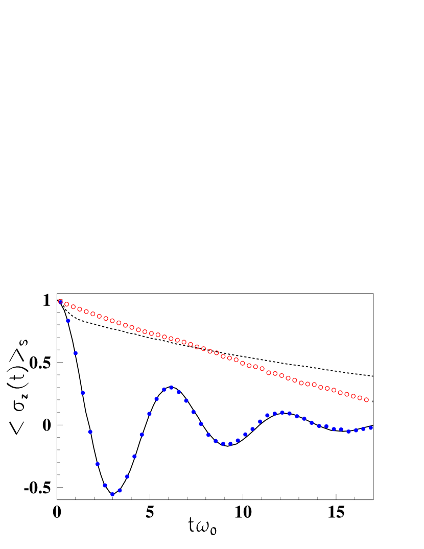
Figure 1: Evolution of $\left\langle\sigma_{z}(t)\right\rangle_{S}$ (assuming $\left\langle\sigma_{z}(0)\right\rangle_{S}=1$) as a function of time obtained through the average of paths simulated with Eq. (23) with the Markovian process described by Eqs. (29-33) and memory functions given by Eq. (34-35). We assume that $\displaystyle J(\omega)=\eta\omega\frac{\Delta^{2}_{c}}{\Delta^{2}_{c}+\omega^{2}}$. Two sets of parameters are used. In both cases, $\Delta_{c}=5\omega_{0}$, $k_{B}T=2\hbar\omega_{0}$ and $\hbar\varepsilon=0$. The filled and open circles correspond respectively to $\pi\eta=0.2\hbar\omega_{0}$ and $\pi\eta=4\hbar\omega_{0}$ and are compared respectively with the solid and dashed line obtained with the same set of parameters in Fig. 2 of ref. Yan et al. (2004). Results are obtained with $2\times 10^{4}$ trajectories.

Fig. 1 shows examples of dynamical evolution of $\overline{\langle\sigma_{z}(t)\rangle_{S}}$ obtained using Eq. (23) and averaging over stochastic trajectories both for weak (filled circle) and strong (open circle) coupling. Results are compared with the Hierarchical approach proposed in ref. Yan et al. (2004). This deterministic approach provides an alternative a priori exact formulation of open quantum systems dynamics and was originally motivated by numerical difficulties encountered in the stochastic theory proposed in ref. Shao (2004). Such difficulties do not occur in the present simulation and much less stochastic trajectories seem to be needed to accurately describe the dynamical evolution. Only $2\times 10^{4}$ trajectories have been used to obtained Fig. 1 leading to statistical errors close to zero (for comparison see discussion in Zhou et al. (2005)). The computer time for the two figures was less than an hour for the weak coupling case up to several hours for the strong coupling case on a standard personal computer. The difference in computing time comes from the fact that smaller numerical time step should be used as the coupling strength increases to achieve good numerical accuracy, the main difficulty being to properly evaluate time integrals in Eq. (24). Denoting the time step by $\Delta t$, $\Delta t\omega_{0}=1.2\times 10^{-3}$ and $\Delta t\omega_{0}=2.2\times 10^{-4}$ have been used for weak and strong coupling respectively.

In the weak coupling case, results of our stochastic scheme displayed in Fig. 1 (filled circles) perfectly match the result of ref. Yan et al. (2004) (solid line). In contrary to ref. Zhou et al. (2005), statistical errors remain small even for long time evolution. The difference in numerical accuracy can be assigned to the second term in Eq. (24) which turns out to be crucial for numerical implementation. Stochastic simulations for strong coupling parameters (open circles) slightly differ from the results obtained with the hierarchical approach in ref. Yan et al. (2004). The numerical convergence of the stochastic simulation presented in Fig. 1 has been checked. Therefore, the difference might be due to the fact that the numerical accuracy depends on the truncation scheme used in the hierarchy, even though the method of ref. Yan et al. (2004) is exact.

III.3 Comparison with the Time-convolutionless method (TCL)

The possibility to simulate exactly the system dynamics can also serve as a benchmark for other methods. For instance, we compared the exact stochastic scheme with the approximate Time-Convolutionless (TCL) projection operator method of ref. Breuer et al. (1999); Breuer and Petruccione (2002). Figure 2 presents the results of the exact stochastic simulation compared with the TCL2 method applied to the spin-boson model in ref. Breuer et al. (1999). In this figure different cases corresponding to either low or high temperature regime and weak or strong coupling are presented. We see that the best agreement is obtained in the weak coupling and high temperature case. In general, the TCL2 method compares well with the exact simulation if the coupling is rather small. As the coupling increases (lower panels of figure 2), the difference between the TCL technique and the exact method increases. Note that the TCL method seems to systematically underestimate the damping. Note finally that the use of TCL4 equations instead of TCL2 does not improve the comparison.

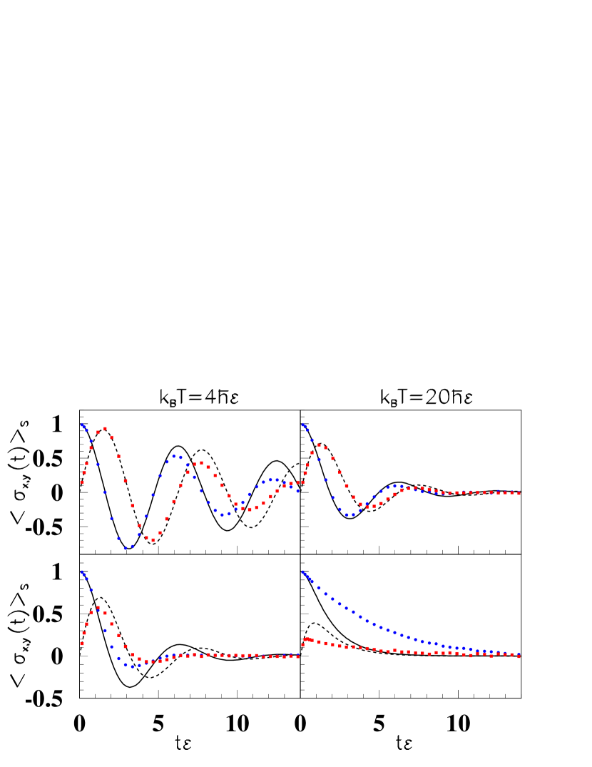
Figure 2: Average evolution of $\left\langle\sigma_{x}(t)\right\rangle_{S}$ (filled circles) and $\left\langle\sigma_{y}(t)\right\rangle_{S}$ (filled squares) as a function of time. The initial condition correspond to $\left\langle\sigma_{x}(0)\right\rangle_{S}=1$. In all cases, $\hbar\omega_{0}=0$ and $\Delta_{c}=10\varepsilon$. $k_{B}T=4\hbar\varepsilon$ and $k_{B}T=20\hbar\varepsilon$ are used respectively for calculations presented in the left and right column. In both cases, upper panels present results for weak coupling ($\pi\eta=0.2\hbar\varepsilon$) while in lower panels a stronger coupling is considered ($\pi\eta=1.0\hbar\varepsilon$). Simulations have been performed with $4\times 10^{4}$ trajectories. For all cases, dynamical evolutions of the $x$ and $y$ spin components obtained with the TCL2 method Breuer et al. (1999); Breuer and Petruccione (2002) are displayed by solid and dashed lines respectively.

III.4 Discussion of approximate system evolution obtained with real noise and Hermitian system densities in stochastic evolution

Applications presented above use specific constraints on the Markovian process given by Eqs. (33). This prescription greatly simplifies stochastic calculus. For instance, simple exact expressions have been obtained for $D(t,s)$ and $D_{1}(t,s)$ when the system is coupled to a heat-bath of harmonic oscillators (Eqs. (34-35)). The main consequence of Eqs. (33) is that $du_{S/E}$ and $dv_{S/E}$ should be complex stochastic variables leading to non Hermitian densities along paths. As illustrated above, such a stochastic process could be used to simulate exactly the reduced density evolution. The main disadvantage of non-Hermitian densities is however that system observables could hardly be interpreted. We discuss here the possibility to perform stochastic evolution of reduced Hermitian densities.

Relaxing the constraints given by Eqs. (33), authorizes to choose $du_{S/E}$ and $dv_{S/E}$ as real stochastic variables, which automatically insures that $\rho_{S}(t)$ and $\rho_{E}(t)$ remain hermitian. This alternative has however two major drawbacks. First, one cannot anymore have an equivalent SSE picture. Second, while $D(t,s)$ still identifies with Eq. (34), no simple exact expression can be worked out for $D_{1}(t,s)$. However, since this kernel is a functional of $\rho_{E}(s)$, a hierarchy of more and more accurate approximations could be obtained by successive replacements of $\rho_{E}(s)$ into Eq. (25) by its integral expression, Eq. (22). In the present work, we concentrate on the simplest case where $\rho_{E}(s)$ is replaced by $\rho_{E}(s)\simeq U_{E}(t,t_{0})\rho_{E}(t_{0})U^{\dagger}_{E}(t,t_{0})$ in the time integral of the memory kernel. In this limit, $D_{1}(s,t)$ also reduces to Eq. (35). By doing this approximation, the stochastic process is not exact anymore. Fig. 3 presents a comparison of the exact stochastic simulation obtain with complex noise (filled circles) and the approximate case with real noise (open circles). The parameters of the spin-boson model are the same as in Fig. 1.

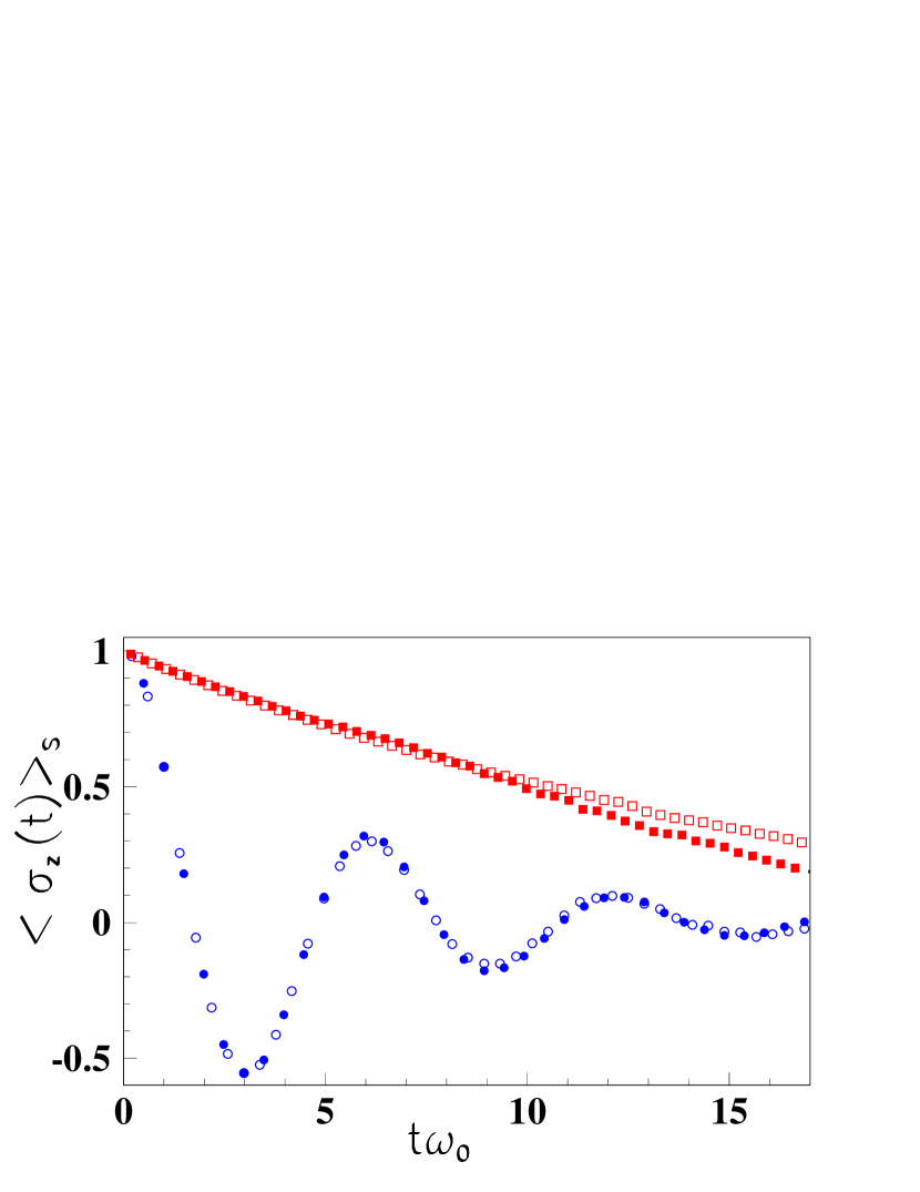
Figure 3: Results obtained in the weak and strong coupling case with the exact stochastic simulation using complex noises and non-hermitian (filled circles) are compared with the approximate simulation (open circles) using real noise and hermitian densities along each paths. In this figure, the values of parameters are the same as in Fig. 1.

This figure shows that the approximate scheme with real noise is very close to the exact simulation even in the strong coupling limit. In the latter case, only at very large time, the two simulation start to deviate slightly from one another. For completeness, approximate stochastic simulations obtained for cases presented in figure 2 are compared to the exact scheme in figure 4. We see that except for the weak coupling and low temperature case, the approximate simulation is very close to the exact case. It is worth mentioning that approximate simulation presented here uses the simplest prescription for $D_{1}(s,t)$. Therefore, improved description could a priori be obtained using better approximation of $D_{1}(s,t)$ obtained with the method described above. This example is very encouraging and provides a new method to simulate open systems with a stochastic process preserving the hermitian properties of the system density.

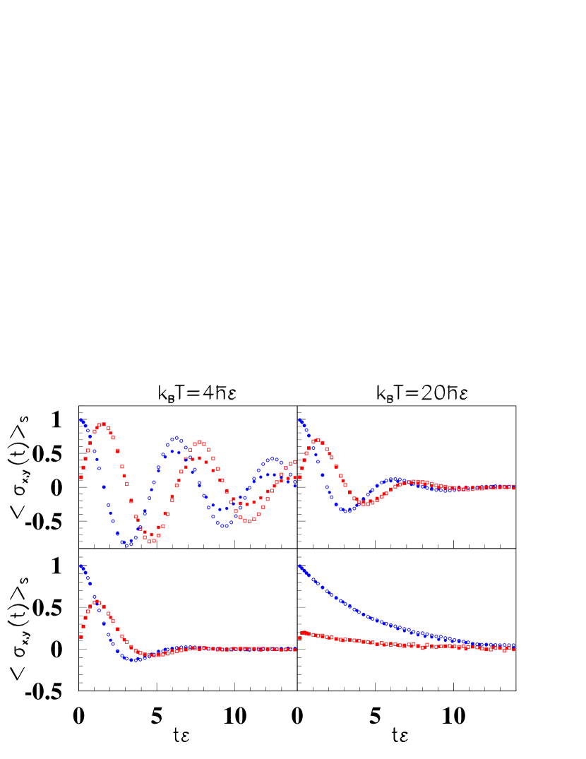
Figure 4: Average evolution of $\left\langle\sigma_{x}(t)\right\rangle_{S}$ (filled circles) and $\left\langle\sigma_{y}(t)\right\rangle_{S}$ (filled squares) as a function of time obtained with the exact stochastic scheme using the same sets of parameters as in figure 2. In each cases, dynamical evolutions of the $x$ and $y$ spin components obtained with the approximate stochastic simulation using real noise are respectively displayed with open circles and open squares.

IV Conclusion

The results obtained with the stochastic theory for the spin-boson model are very encouraging. The theory turns out to be accurate not only to simulate short but also long-time dynamics and does not seem to suffer from numerical instability quoted in ref Zhou et al. (2005). It is worth mentioning that optimization techniques proposed in ref. Lacroix (2005) which are not used here, can be implemented to further reduce the number of stochastic paths. Besides the numerical aspects, the link with classical dissipations dynamics could be easily made, similarly to ref. Stockburger and Grabert (2002).

Our stochastic approach could be generalized to any initial conditions that could be written as a mixing of separable densities, i.e. $D(t_{0})=\sum_{n}W_{n}D^{(n)}(t_{0})$ with $D^{n}=\rho^{n}_{S}\otimes\rho^{n}_{E}$ where the $W_{n}$ are complex coefficients. Then, the complete exact dynamics is recovered by both averaging over trajectories starting from each $D^{(n)}(t=0)$ individually and averaging over the initial conditions. The theory is also not restricted to real time evolution. Statistical properties of the system+environment could be studied by considering imaginary time propagation, i.e. $idt/\hbar\rightarrow\beta$. Imaginary time propagations lead naturally to densities written as a mixing of separable densities and could then serve as initial conditions for real time evolution. By combining both imaginary time and real time propagation, general physical problems similar to those depicted in ref. Stockburger and Grabert (2002) can be addressed. The main limitation of the technique is clearly the choice of coupling operator $\mathbf{B}$ which should give simple memory functions (Eq. (25 - 26)). It is however worth mentioning that most of the coupling operators used in the context of open quantum systems already enter into this category Carmichael (1993); Weiss (1999); Gardiner and Zoller (2000); Breuer and Petruccione (2002). We believe that the stochastic theory presented in this paper can be a valuable tool to access exactly the dynamics of more complex open quantum systems. We presented here specific applications on systems coupled to a heat-bath. The approach can however be applied to various types of environments and couplings which might be of great interest to address dissipation, measurement and/or decoherence problems in quantum systems.

Appendix A Proof of Eq. (24) for a heat-bath of Harmonic oscillators

We give here a proof of Eq. (24) where $D$ and $D_{1}$ identify with Eqs. (34-35). The environment is assumed to be a set of harmonic oscillators, labeled by ”$n$” associated to creation/annihilation ($a^{\dagger}_{n}$,$a_{n}$), i.e.

$$H=\sum_{n}\hbar\omega_{n}\left(a^{\dagger}_{n}a_{n}+\frac{1}{2}\right).$$ (41)

If thermal equilibrium is initially assumed, the environment density writes as a product of densities of each oscillator, $\rho_{E}=\Pi_{n}\rho_{n}$ where each density can be written as Gaussian operators (see for instance Gardiner and Zoller (2000)) determined by first and second moments of the $(a^{\dagger}_{n},a_{n})$. The time evolution of the environment is given by Eq. (16) where $\mathbf{B}\equiv-\sum_{n}\kappa_{n}x_{n}$ and where the fluctuating variables verify (according to Eq. (33)):

$$\overline{d\lambda_{E}d\lambda_{E}}=\overline{d\xi_{E}d\xi_{E}}=\overline{d\lambda_{E}d\xi_{E}}=0.$$ (42)

Above prescription and the specific form of $\mathbf{B}$ induces important simplifications listed below. First, the initial product form of the environment density is preserved along the stochastic paths where each oscillator density verifies ${\rm Tr}(\rho_{n})=1$ and where for each pairs of densities $d(\rho_{n}\rho_{m})=\rho_{n}d\rho_{m}+d\rho_{n}\rho_{m}$. Second, due to the linear coupling operator, the Gaussian nature of initial densities is also preserved along paths. Therefore, we can equivalently solve the density equation of motion or follow first and second moments of each $(a^{\dagger}_{n},a_{n})$ in time. Here we consider the second strategy.

From the $\rho_{E}$ evolution, the equation of motion of each pairs $\langle a^{\dagger}_{n}\rangle={\rm Tr}(\rho_{E}a^{\dagger}_{n})$ and $\langle a_{n}\rangle={\rm Tr}(\rho_{E}a_{n})$ reads:

$$d\left\langle a_{n}\right\rangle = -i\omega_{n}dt\left\langle a_{n}\right\rangle+\frac{dt}{i\hbar}c_{n}\left\langle{\mathbf{Q}}\right\rangle+c_{n}\left\{d\xi_{E}\left(\sigma^{(n)}_{+-}(t)+\sigma^{(n)}_{--}(t)+1\right)+d\lambda_{E}\left(\sigma^{(n)}_{+-}(t)+\sigma^{(n)}_{--}(t)\right)\right\},$$ (43)

$$d\left\langle a^{\dagger}_{n}\right\rangle = +i\omega_{n}dt\left\langle a^{\dagger}_{n}\right\rangle-\frac{dt}{i\hbar}c_{n}\left\langle{\mathbf{Q}}\right\rangle+c_{n}\left\{d\xi_{E}\left(\sigma^{(n)}_{+-}(t)+\sigma^{(n)}_{++}(t)\right)+d\lambda_{E}\left(\sigma^{(n)}_{+-}(t)+\sigma^{(n)}_{++}(t)+1\right)\right\},$$

where we have introduced the notation $c_{n}\equiv-\kappa_{n}/\sqrt{2\eta_{n}}$ and $\eta_{n}=m_{n}\omega_{n}/\hbar$. Here, $\sigma^{(n)}_{++}$, $\sigma^{(n)}_{--}$ and $\sigma^{(n)}_{+-}$ denote the second moments of the $a^{\dagger}_{n}$, $a_{n}$ operators:

$$\sigma_{+-}^{(n)} \equiv \left\langle a^{\dagger}_{n}a_{n}\right\rangle-\left\langle a_{n}\right\rangle\left\langle a^{\dagger}_{n}\right\rangle=\sigma_{-+}^{(n)}-1,$$

$$\sigma_{--}^{(n)} \equiv \left\langle a_{n}a_{n}\right\rangle-\left\langle a_{n}\right\rangle\left\langle a_{n}\right\rangle,$$

$$\sigma_{++}^{(n)} \equiv \left\langle a^{\dagger}_{n}a^{\dagger}_{n}\right\rangle-\left\langle a^{\dagger}_{n}\right\rangle\left\langle a^{\dagger}_{n}\right\rangle.$$

According to the stochastic environment dynamics, we can show that these moments simply evolve as

$$\left\{\begin{array}[]{lll}d\sigma^{(n)}_{--}&=&-2i\omega_{n}dt\sigma^{(n)}_{--},\\ d\sigma^{(n)}_{++}&=&+2i\omega_{n}dt\sigma^{(n)}_{++},\\ d\sigma^{(n)}_{+-}&=&0.\end{array}\right.$$ (47)

Since we assume that each oscillator is initially at thermal equilibrium, we deduce that second moments are constant in time with $\sigma^{(n)}_{--}(t)=\sigma^{(n)}_{++}(t)=0$, while $\sigma^{(n)}_{-+}(t)=\sigma^{(n)}_{+-}+1=(\bar{N}(\omega_{n})+1)$. Here, we have introduced the standard function Gardiner and Zoller (2000): $(2\bar{N}(\omega_{n})+1)=\coth\left(\hbar\omega_{n}/(2k_{B}T)\right)$. Substituting in Eqs. (43-A) and using standard integration techniques Breuer and Petruccione (2002) leads finally to

$$\left\langle a_{n}(t)\right\rangle=e^{-i\omega_{n}t}\left\langle a_{n}(0)\right\rangle+\frac{c_{n}}{i\hbar}\int_{0}^{t}e^{-i\omega_{n}(t-s)}\left\langle{\mathbf{Q}}(s)\right\rangle ds+c_{n}\int_{0}^{t}e^{-i\omega_{n}(t-s)}\left\{d\xi_{E}(s)\left(\bar{N}(\omega_{n})+1\right)+d\lambda_{E}(s)\bar{N}(\omega_{n})\right\},$$

$$\left\langle a^{\dagger}_{n}(t)\right\rangle=e^{+i\omega_{n}t}\left\langle a^{\dagger}_{n}(0)\right\rangle-\frac{c_{n}}{i\hbar}\int_{0}^{t}e^{+i\omega_{n}(t-s)}\left\langle{\mathbf{Q}}(s)\right\rangle ds+c_{n}\int_{0}^{t}e^{+i\omega_{n}(t-s)}\left\{d\xi_{E}(s)\bar{N}(\omega_{n})+d\lambda_{E}(s)(\bar{N}(\omega_{n})+1)\right\}.$$ (48)

Accordingly, each position operator entering in $\left\langle{\mathbf{B}}(t)\right\rangle$ reads:

$$\left\langle x_{n}(t)\right\rangle = \frac{1}{\sqrt{2\eta_{n}}}\Big{\{}\left\langle a_{n}(0)\right\rangle e^{-i\omega_{n}t}+\left\langle a^{\dagger}_{n}(0)\right\rangle e^{+i\omega_{n}t}\Big{\}}+\frac{\kappa_{n}}{\hbar\eta_{n}}\int^{t}_{0}\sin(\omega_{n}[t-s])\left\langle{\mathbf{Q}}(s)\right\rangle ds,$$

$$-\frac{\kappa_{n}}{2\eta_{n}}\int^{t}_{0}\left\{\cos(\omega_{n}[t-s])(2\bar{N}(\omega_{n})+1)\left[d\xi_{E}(s)+d\lambda_{E}(s)\right]-i\sin(\omega_{n}[t-s])\left[d\xi_{E}(s)-d\lambda_{E}(s)\right]\right\}.$$

Assuming the initial conditions $\left\langle a_{n}(0)\right\rangle=\left\langle a^{\dagger}_{n}(0)\right\rangle=0$, substituting in the expression of $\left\langle{\mathbf{B}}(t)\right\rangle=-\sum_{n}\kappa_{n}\left\langle x_{n}(t)\right\rangle$ and introducing the spectral density (Eq. (36)), we finally recover equation (24) where $D$ and $D_{1}$ are respectively given by Eqs. (34) and (35).

References

• Weiss (1999) U. Weiss, Quantum Dissipative Systems (World Scientific, Singapore, 2nd ed., 1999).
• Breuer and Petruccione (2002) H. Breuer and F. Petruccione, The Theory of Open Quantum Systems (Oxford University Press, Oxford, 2002).
• Joos et al. (2003) E. Joos, H. Zeh, C. Kiefer, D. Giulini, J. Kupsch, and I.-O. Stamatescu, Decoherence and the Appearance of a Classical World in Quantum Theory (Springer, New York, 2003).
• Plenio and Knight (1998) M. B. Plenio and P. L. Knight, Rev. Mod. Phys. 70, 101 (1998).
• Stockburger and Grabert (2002) J. T. Stockburger and H. Grabert, Phys. Rev. Lett. 88, 170407 (2002).
• Dalibard et al. (1992) J. Dalibard, Y. Castin, and K. Mølmer, Phys. Rev. Lett. 68, 580 (1992).
• Dum et al. (1992) R. Dum, P. Zoller, and H. Ritsch, Phys. Rev. A 45, 4879 (1992).
• Gisin and Percival (1992) N. Gisin and I. Percival, J. Math. Phys. A25, 5677 (1992).
• Carmichael (1993) H. Carmichael, An Open Systems Approach to Quantum Optics (Lecture Notes in Physics, Springer-Verlag, Berlin, 1993).
• Castin and Mo/lmer (1996) Y. Castin and K. Mo/lmer, Phys. Rev. A 54, 5275 (1996).
• Rigo and Gisin (1996) M. Rigo and N. Gisin, Quantum Semiclass. Opt. 8, 255 (1996).
• Gardiner and Zoller (2000) W. Gardiner and P. Zoller, Quantum Noise (Springer-Verlag, Berlin-Heidelberg, 2000).
• Breuer et al. (1999) H.-P. Breuer, B. Kappler, and F. Petruccione, Phys. Rev. A 59, 1633 (1999).
• Breuer et al. (2001) H.-P. Breuer, B. Kappler, and F. Petruccione, Ann. Phys. 291, 36 (2001).
• Diósi and Strunz (1996) L. Diósi and W. T. Strunz, Phys. Lett. A224, 25 (1996).
• Diósi et al. (1998) L. Diósi, N. Gisin, and W. T. Strunz, Phys. Rev. A 58, 1699 (1998).
• Strunz et al. (1999) W. T. Strunz, L. Diósi, and N. Gisin, Phys. Rev. Lett. 82, 1801 (1999).
• Strunz (2005) W. T. Strunz, New Journ. of Phys. 7, 91 (2005).
• Shao (2004) J. Shao, J. Chem. Phys. 120, 5053 (2004).
• Breuer (2004a) H.-P. Breuer, Eur.Phys.J. D 29, 105 (2004a).
• Lacroix (2005) D. Lacroix, Phys. Rev. A 72, 013805 (2005).
• Breuer et al. (2004) H.-P. Breuer, D. Burgarth, and F. Petruccione, Phys. Rev. B 70, 045323 (2004).
• Breuer (2004b) H.-P. Breuer, Physical Review A 69, 022115 (2004b).
• Zhou et al. (2005) Y. Zhou, Y. Yan, and J. Shao, Europhys. Lett. 3, 334 (2005).
• Breuer and Petruccione (2007) H.-P. Breuer and F. Petruccione, Phys. Rev. E 76, 016701 (2007).
• Gardiner (1985) W. Gardiner, Handbook of Stochastic Methods (Springer-Verlag, Berlin-Heidelberg, 1985).
• Lacroix (2007) D. Lacroix, Ann. of Phys. 322, 2055 (2007), eprint quant-ph/0606246.
• Feynman and Vernon (1963) R. P. Feynman and J. Vernon, F. L., Ann. Phys. 24, 118 (1963).
• Caldeira and Leggett (1983) A. O. Caldeira and A. J. Leggett, Ann. Phys. 149, 374 (1983).
• Yan et al. (2004) Y. Yan, F. Yang, Y. Liu, and J. Shao, Chem. Phys. Lett. 395, 216 (2004).
• Leggett et al. (1987) A. J. Leggett, S. Chakravarty, A. T. Dorsey, M. P. A. Fisher, A. Garg, and W. Zwerger, Rev. Mod. Phys. 59, 1 (1987).
• Egger and Mak (1994) R. Egger and C. H. Mak, Phys. Rev. B 50, 15210 (1994).