Genuine tripartite entanglement monotone of $(2\otimes 2\otimes n)-$dimensional systems

Abstract

A genuine tripartite entanglement monotone is presented for $(2\otimes 2\otimes n)$-dimensional tripartite pure states by introducing a new entanglement measure for bipartite pure states. As an application, we consider the genuine tripartite entanglement of the ground state of the exactly solvable isotropic spin-$\frac{1}{2}$ chain with three-spin interaction. It is shown that the singular behavior of the genuine tripartite entanglement exactly signals a quantum phase transition.

I Introduction

The existence of quantum entanglement is a joint consequence of the superposition principle and the tensor product structure of the quantum mechanical state space of composite quantum systems. Entanglement is a remarkable feature that distinguishes the quantum from the classical world. One of the main tasks of quantum entanglement theory is to quantitively characterize the extent to which composite quantum systems are entangled by constructing a mathematical function——an entanglement measure that should be an entanglement monotone, or in other words, not increase on averaging under local operations and classical communications (LOCC). Even though many efforts have been applied to a variety of quantum systems [1-3], only bipartite pure-state and low-dimensional systems are well understood. The quantification of entanglement for high-dimensional systems and multipartite quantum systems remains an open question.

An important step in studying multipartite entanglement was taken by Coffman, Kundu and Wootters [4]. They showed that a quantum state has only a limited shareability for quantum entanglement, when they introduced the so-called residual entanglement for tripartite systems of qubits based on the remarkable concurrence [1] to measure an essential three-qubit (three-way) entanglement which must be shared by all the three qubits. A representative example with such a property is the Greenberger-Horne-Zeilinger (GHZ) state which has maximal residual entanglement. Once a qubit is traced out, the remaining two qubits are separable. Later, it was shown that this essential three-qubit entanglement is one (GHZ-type) of the two inequivalent classes (GHZ-type and W-type) of tripartite entanglement of qubits [5]. In this paper, we call it genuine tripartite entanglement. For a general multipartite quantum state, multipartite quantum entanglement can be classified into much more inequivalent entanglement classes [6-9], which is also one principal reason why the entanglement in multipartite systems is much more complicated. Therefore, in general a single quantity can not effectively and thoroughly measure multipartite entanglement. However, sometimes a single quantity is quite convenient and straightforward if one is going to study the separability property of a given quantum system [10-12], or collect the contributions of some entanglements of different classes as a whole [13-16], or more naturally, measure entanglement of a given class [6-9].

In this paper, we introduce a single quantity to characterize the genuine tripartite entanglement of tripartite $(2\otimes 2\otimes n)-$dimensional quantum systems based on a new bipartite entanglement measure. The distinct advantage is that the quantity is not only an entanglement monotone, but also explicitly quantifies the GHZ-type inseparability of a tripartite high-dimensional pure state. As an application, we consider the genuine tripartite entanglement of the ground state of the exactly solvable isotropic spin-$\frac{1}{2}$ chain with three-spin interaction [17,18]. It is shown that the singularity of the genuine tripartite entanglement exactly signals a quantum phase transition. The paper is organized as follows. First, we introduce a new bipartite entanglement monotone; and then we give the genuine tripartite entanglement monotone and consider the entanglement of the ground state of the exactly solvable isotropic spin-$\frac{1}{2}$ chain with three-spin interaction; the conclusions are drawn at the end.

II A new entanglement monotone for bipartite pure states

As we know, a bipartite quantum pure state $\left|\psi\right\rangle_{AB}$ defined in $\left(n_{1}\otimes n_{2}\right)$ dimension is, in general, considered as a vector, i.e. $\left|\psi\right\rangle_{AB}=[a_{00},a_{01},\cdot\cdot\cdot,a_{0n_{2}},a_{10},a_{11},\cdot\cdot\cdot,a_{n_{1}n_{2}}]^{T}$ with superscript $T$ denoting transpose operation. But in a different notation, $\left|\psi\right\rangle_{AB}$ can also be written in matrix form as

$$\psi_{AB}=\left(\begin{array}[]{cccc}a_{00}&a_{01}&\cdots&a_{0n_{2}}\\ a_{10}&a_{11}&\cdots&a_{1n_{2}}\\ \vdots&\vdots&\ddots&\vdots\\ a_{n_{1}0}&a_{n_{1}1}&\cdots&a_{n_{1}n_{2}}\end{array}\right),$$ (1)

by which one can easily find the reduced density matrix

$$\rho_{A}=\psi_{AB}\psi_{AB}^{{\dagger}}.$$ (2)

Let $\sigma_{i}$, $i=1,2,\cdots,\mathcal{D}$, with $\mathcal{D}=\min\{n_{1},n_{2}\},$be the singular values of $\psi_{AB}$ or the square roots of eigenvalues of $\rho_{A}$ in decreasing order. Define

$$\mathcal{S}\left(\rho_{A}\right)=\left(\sum\limits_{i=1}^{\mathcal{D}}\sqrt{\sigma_{i}}\right)^{2},$$ (3)

then $E(\left|\psi\right\rangle_{AB})\$is defined by

$$E(\left|\psi\right\rangle_{AB})=\mathcal{N}\left[\mathcal{S}\left(\rho_{A}\right)-1\right]$$ (4)

with $\mathcal{N}$ an adjustable constant by which one can select different reference frames. For example, one can set $\mathcal{N=}\frac{2\sqrt{2}+1}{7}$ such that $E=1$ for Bell states and $\mathcal{N=}\frac{\mathcal{D}\sqrt{\mathcal{D}}+1}{\mathcal{D}^{3}-1}$ such that $E=1$ for $\mathcal{D}$-dimensional maximal entangled states.

Theorem 1. $E(\left|\psi\right\rangle_{AB})$ is an entanglement measure of $\left|\psi\right\rangle_{AB}$.

Proof. It is obvious that $\mathcal{S}\left(\rho_{A}\right)=1$ (the rank of $\psi_{AB}$ is one) if $\left|\psi\right\rangle_{AB}$ is separable, i.e., $E(\left|\psi\right\rangle_{AB})=0$. Conversely, if $E(\left|\psi\right\rangle_{AB})=0$, $\mathcal{S}\left(\rho_{A}\right)=1$ which implies that the rank of $\psi_{AB}$ is one, i.e., $\left|\psi\right\rangle_{AB}$ is separable. These results show that $E(\left|\psi\right\rangle_{AB})=0$ is a sufficient and necessary condition for separability. In fact, it is equivalent to the separability in terms of the Schmidt decomposition.

Now, we show that $E(\left|\psi\right\rangle_{AB})$ is an entanglement monotone, i.e., $E(\left|\psi\right\rangle_{AB})$ does not increase under LOCC operations. At first, it is easily found that $E(\left|\psi\right\rangle_{AB})$ does not change under local unitary transformations because the singular values of $\psi_{AB}$ are invariant under such transformations. Next, without loss of generality, we suppose that the local operations are only performed on the subsystem $A$. Furthermore, for simplicity, we assume a local unitary transformation $Z$ is performed on subsystem $A$ beforehand. This is valid because local unitary transformations do not change the entanglement. Analogously to Ref. [5], let $A_{1}$ and $A_{2}$ be two Positive-Operator-Value-Measurement (POVM) elements such that $A_{1}^{{\dagger}}A_{1}+A_{2}^{{\dagger}}A_{2}=\mathbf{1}_{A}$, with $\mathbf{1}_{A}$ denoting the identity of subsystem $A$ and $A_{i}=U_{i}D_{i}V$, where $U_{i}$ and $V$ are unitary matrices and $D_{i}$ are diagonal matrices with entries $(a_{1},a_{2},\cdots)$ and $[\sqrt{1-a_{1}^{2}},\sqrt{1-a_{2}^{2}},\cdots]$, respectively. For some initial state $\left|\psi\right\rangle_{AB}$, let $\left|\theta_{i}\right\rangle=(A_{i}Z\otimes\mathbf{1}_{B})\left|\psi\right\rangle_{AB}$ be the unnormalized states obtained after the POVM operations. The corresponding normalized states can be given by $\left|\theta_{i}^{\prime}\right\rangle=\left|\theta_{i}\right\rangle/\sqrt{p_{i}}$, where $p_{i}=\left\langle\theta_{i}\right|\left.\theta_{i}\right\rangle$. Then the average entanglement after operations can be given by

$$\left\langle E(\left|\psi\right\rangle_{AB})\right\rangle=p_{1}E(\left|\theta_{1}^{\prime}\right\rangle)+p_{2}E(\left|\theta_{2}^{\prime}\right\rangle).$$ (5)

In matrix notation, $\left|\theta_{i}\right\rangle$ can be rewritten by $\theta_{i}=A_{i}Z\psi_{AB}$. $E(\left|\theta_{i}^{\prime}\right\rangle)$ can be rewritten as

$$E(\left|\theta_{i}^{\prime}\right\rangle)=E(U_{i}D_{i}VZY\Lambda W^{{\dagger}}/\sqrt{p_{i}}),$$ (6)

where $\psi_{AB}=Y\Lambda W^{{\dagger}}$ is the singular value decomposition of $\psi_{AB}$. Since $E$ is invariant under local unitary transformations and we select $Z=V^{{\dagger}}Y^{{\dagger}}$ for simplicity, eq. (6) can be explicitly given by

$$E(\left|\theta_{1}^{\prime}\right\rangle)=\mathcal{N}\left[\frac{1}{\sqrt{p_{1}}}\left(\sum\limits_{k=1}^{\mathcal{D}}\sqrt{a_{k}\sigma_{k}}\right)^{2}-1\right].$$ (7)

Similarly,

$$E(\left|\theta_{2}^{\prime}\right\rangle)=\mathcal{N}\left[\frac{1}{\sqrt{p_{2}}}\left(\sum\limits_{k=1}^{\mathcal{D}}\sqrt{\sqrt{1-a_{k}^{2}}\sigma_{k}}\right)^{2}-1\right].$$ (8)

Substituting eq. (7) and eq. (8) into eq. (5), $\left\langle E(\left|\psi\right\rangle_{AB})\right\rangle$ can be written as

$$\left\langle E(\left|\psi\right\rangle_{AB})\right\rangle$$ (9)

$$= \mathcal{N}\left[\sqrt{p_{1}}\left(\sum\limits_{k=1}^{\mathcal{D}}\sqrt{a_{k}\sigma_{k}}\right)^{2}+\sqrt{p_{2}}\left(\sum\limits_{k=1}^{\mathcal{D}}\sqrt{\sqrt{1-a_{k}^{2}}\sigma_{k}}\right)^{2}-1\right]$$

$$= \mathcal{N}\left[\sum\limits_{k=1}^{\mathcal{D}}\left(\sqrt{p_{1}}a_{k}+\sqrt{p_{2}}\sqrt{1-a_{k}^{2}}\right)\sigma_{k}\right.$$

$$+\left.\sum\limits_{i\neq j}\left(\sqrt{p_{1}a_{i}a_{j}}+\sqrt{p_{2}\sqrt{\left(1-a_{i}^{2}\right)\left(1-a_{j}^{2}\right)}}\right)\sqrt{\sigma_{i}\sigma_{j}}-1\right]$$

$$\leq \mathcal{N}\left[\left(\sum\limits_{k=1}^{\mathcal{D}}\sqrt{\sigma_{k}}\right)^{2}-1\right]=E(\left|\psi\right\rangle_{AB}),$$

where the inequality follows from $\sqrt{p_{1}}a_{k}+\sqrt{p_{2}}\sqrt{1-a_{k}^{2}}\leq 1$ for any $k$, $\sqrt{p_{1}a_{i}a_{j}}+\sqrt{p_{2}\sqrt{\left(1-a_{i}^{2}\right)\left(1-a_{j}^{2}\right)}}\leq 1$ and $p_{1}^{2}+p_{2}^{2}=1$. Eq. (9) shows that $E$ is an entanglement monotone. $\hfill\Box$

III
Genuine tripartite entanglement monotone for tripartite pure states

Let us focus on a $\left(2\otimes 2\otimes n\right)-$dimensional tripartite quantum pure state $\left|\psi\right\rangle_{ABC}$ defined in the Hilbert space $H_{1}\otimes H_{2}\otimes H_{3}$, the $\left(2\otimes 2\right)$ reduced density matrix of which can be given by

$$\rho_{AB}=tr_{C}\left[\left|\psi\right\rangle_{ABC}\left\langle\psi\right|\right].$$ (10)

Denote the eigenvalue decomposition of $\rho_{AB}$ by

$$\rho_{AB}=\Phi M\Phi^{{\dagger}},$$ (11)

where the columns of $\Phi$ are the eigenvectors of $\rho_{AB}$ and $M$ is a diagonal matrix with the diagonal elements being the eigenvalues of $M$. Define a $4\times 4$ matrix in terms of the spin flip operator $\sigma_{y}\otimes\sigma_{y}$ as

$$\mathcal{M}=\sqrt{M}\Phi^{T}\sigma_{y}\otimes\sigma_{y}\Phi\sqrt{M}.$$ (12)

Then $\mathcal{M}$ can be regarded as an unnormalized pure state given in matrix notation analogous to eq. (1). Therefore, the separability of $\mathcal{M}$ can be characterized by our bipartite entanglement monotone introduced in the previous section. Therefore, we have the following theorem.

Theorem 2.-For a $\left(2\otimes 2\otimes n\right)-$dimensional tripartite quantum pure state $\left|\psi\right\rangle_{ABC}$, the genuine tripartite entanglement measure can be given by

$$E(\left|\psi\right\rangle_{ABC}) = E(\mathcal{M})=\mathcal{\tilde{N}}\left[\mathcal{S}\left(\mathcal{MM}^{\dagger}\right)-\mathcal{F}\left(\mathcal{MM}^{\dagger}\right)\right]$$ (13)

$$= \mathcal{\tilde{N}}\left[\mathcal{S}\left(\rho_{AB}\tilde{\rho}_{AB}\right)-\mathcal{F}\left(\rho_{AB}\tilde{\rho}_{AB}\right)\right]$$ (14)

$$= \mathcal{\tilde{N}}\sum_{i\neq j}\sqrt{\sigma_{i}\sigma_{j}},$$ (15)

where $\tilde{\rho}_{AB}=$ $\left(\sigma_{y}\otimes\sigma_{y}\right)\rho_{AB}^{\ast}\left(\sigma_{y}\otimes\sigma_{y}\right)$,

$$\mathcal{F}\left(\mathcal{MM}^{\dagger}\right)=\sum_{i=1}^{4}\sigma_{i},$$ (16)

with $\sigma_{i}$ being the singular values of $\mathcal{M}$ or the eigenvalues of $\rho_{AB}\tilde{\rho}_{AB}$ and $\tilde{N}$ is an adjustable constant.

Proof. Note that the equivalence between eq. (13) and eq. (14) is implied in Ref. [1] and eq. (15) can be easily derived by substituting $\sigma_{i}$ into eq. (13) or eq. (14).

First of all, we show that $E(\left|\psi\right\rangle_{ABC})$ characterizes the genuine tripartite entanglement. $\left|\psi\right\rangle_{ABC}$ can also be considered as a $\left(4\otimes n\right)$- dimensional bipartite quantum pure state defined in the Hilbert space $\left(H_{1}\otimes H_{2}\right)\otimes H_{3}$. Based on the Schmidt decomposition, one can always select a proper basis such that $\left|\psi\right\rangle_{ABC}=\sum\limits_{i=1}^{4}\alpha_{i}\left|\tilde{\varphi}_{i}\right\rangle\left|\check{\varphi}_{i}\right\rangle,$ where $\left\{\left|\tilde{\varphi}_{i}\right\rangle\right\}$ is the orthogonal and complete basis of subspace $H_{1}\otimes H_{2}$ and $\left\{\left|\check{\varphi}_{i}\right\rangle\right\}$ is the orthogonal and complete basis of a $\left(4\times 4\right)$ -dimensional subspace in $H_{3}$. Select some orthogonal and complete basis of $H_{3}$ that must include $\left\{\left|\check{\varphi}_{i}\right\rangle\right\}$. Then one can construct an $\left(n\times n\right)$- dimensional matrix $\mathcal{\tilde{M}}$ of which $\mathcal{M}$ is a $4\times 4$ block and the rest is zero. Therefore, $\mathcal{\tilde{M}}$ and $\mathcal{M}$ have the same entanglement in terms of our bipartite entanglement measure. Most importantly, the construction of $\mathcal{\tilde{M}}$ is completely consistent with the ’$\mathcal{M}$’ introduced in Ref. [12]. That is to say, the characterization of separability of $\mathcal{M}$ reveals the genuine tripartite entanglement of $\left|\psi\right\rangle_{ABC}$.

Next, we show that $E(\left|\psi\right\rangle_{ABC})$ is an entanglement monotone. We first show that $E(\left|\psi\right\rangle_{ABC})$ does not increase under LOCC in party $A$ only, due to the invariance of the permutation of party $A$ and $B$. Analogously to Ref. [5] and the analysis in the previous section, we again consider a sequence of two-outcome POVM’s. Let $\tilde{A}_{1}$ and $\tilde{A}_{2}$ be two POVM elements such that $\tilde{A}_{1}^{{\dagger}}\tilde{A}_{1}+\tilde{A}_{2}^{{\dagger}}\tilde{A}_{2}=\mathbf{1}_{2}$, then $\tilde{A}_{i}=\tilde{U}_{i}\tilde{D}_{i}\tilde{V}$, where $\tilde{U}_{i}$ and $\tilde{V}$ are unitary matrices and $\tilde{D}_{i}$ are diagonal matrices with entries $(a,b)$ and $[\sqrt{1-a^{2}},\sqrt{1-b^{2}}]$, respectively. For an initial tripartite pure state $\left|\Psi\right\rangle$, let $\left|\Theta_{i}\right\rangle=(A_{i}\otimes\mathbf{1}_{2}\otimes\mathbf{1}_{n})\left|\Psi\right\rangle$ be the unnormalized states obtained after the POVM operations. The corresponding normalized states can be given by $\left|\Theta_{i}^{\prime}\right\rangle=\left|\Theta_{i}\right\rangle/\sqrt{p_{i}^{\prime}}$, where $p_{i}^{\prime}=\left\langle\Theta_{i}\right|\left.\Theta_{i}\right\rangle$. Then

$$\left\langle E(\left|\Psi\right\rangle)\right\rangle=p_{1}^{\prime}E(\left|\Theta_{1}^{\prime}\right\rangle)+p_{2}^{\prime}E(\left|\Theta_{2}^{\prime}\right\rangle).$$ (17)

Substituting $\left|\Theta_{i}^{\prime}\right\rangle$ into eq. (14), one quickly obtains

$$\left\langle E(\left|\Psi\right\rangle)\right\rangle = abE(\left|\Psi\right\rangle)+\sqrt{\left(1-a^{2}\right)\left(1-b^{2}\right)}E(\left|\Psi\right\rangle)$$ (18)

$$\leq E(\left|\Psi\right\rangle).$$

Now, we analogously let $\hat{A}_{1}$ and $\hat{A}_{2}$ be two POVM elements performed on subsystem $C$ such that $\hat{A}_{1}^{{\dagger}}\hat{A}_{1}+\hat{A}_{2}^{{\dagger}}\hat{A}_{2}=\mathbf{1}_{C}$, and $\hat{A}_{i}=\hat{U}_{i}\hat{D}_{i}\hat{V}$, where $\hat{U}_{i}$ and $\hat{V}$ are unitary matrices and $\hat{D}_{i}$ are diagonal matrices with entries $(\tilde{a}_{1},\tilde{a}_{2},\cdots)$ and $[\sqrt{1-\tilde{a}_{1}^{2}},\sqrt{1-\tilde{a}_{2}^{2}},\cdots]$, respectively. At the same time, we also suppose that $\hat{Z}_{i}$ is a local unitary transformation performed on subsystem $C$ after the operation of $\hat{A}_{i}$. For some initial state $\left|\hat{\Psi}\right\rangle$, let $\left|\hat{\Theta}_{i}\right\rangle=(\mathbf{1}_{A}\otimes\mathbf{1}_{B}\otimes\hat{Z}_{i}\hat{A}_{i})\left|\hat{\Psi}\right\rangle$ be the unnormalized states obtained after the POVM operations. The corresponding normalized states can be given by $\left|\hat{\Theta}_{i}^{\prime}\right\rangle=\left|\hat{\Theta}_{i}\right\rangle/\sqrt{p_{i}^{\prime\prime}}$, where $p_{i}^{\prime\prime}=\left\langle\hat{\Theta}_{i}\right|\left.\hat{\Theta}_{i}\right\rangle$. Then

$$\left\langle E(\left|\hat{\Psi}\right\rangle)\right\rangle=p_{1}^{\prime\prime}E(\left|\hat{\Theta}_{1}^{\prime}\right\rangle)+p_{2}^{\prime\prime}E(\left|\hat{\Theta}_{2}^{\prime}\right\rangle).$$ (19)

It has been proved in Ref. [12] that any local operation $Q$ performed on party $C$ of $\left|\hat{\Psi}\right\rangle$ can be equivalently described using the $\left(n\times n\right)$- dimensional symmetric $\mathcal{\tilde{M}}$ of $\left|\hat{\Psi}\right\rangle$ (the nonzero elements are only limited in a $4\times 4$ block $\mathcal{M}$) given by

$$\mathcal{\hat{M}=}Q^{T}\mathcal{\tilde{M}}^{T}Q.$$ (20)

Therefore, after these local operations $E(\left|\hat{\Theta}_{i}^{\prime}\right\rangle)$ is given by

$$E(\left|\hat{\Theta}_{i}^{\prime}\right\rangle)=E\left[\frac{\hat{V}^{T}\hat{D}_{i}^{T}\hat{U}_{i}^{T}\hat{Z}_{i}^{T}\hat{Y}\hat{\Lambda}\hat{Y}^{T}\hat{Z}_{i}\hat{U}_{i}\hat{D}_{i}\hat{V}}{p_{i}^{\prime\prime}}\right],$$ (21)

where $\mathcal{\tilde{M}}=\hat{Y}\hat{\Lambda}\hat{Y}^{T}$ is the singular value decomposition of $\mathcal{\tilde{M}}$. For simplicity, select $Z_{i}=Y^{\ast}U_{i}^{{\dagger}}$, then eq. (21) can be explicitly given by

$$E(\left|\hat{\Theta}_{1}^{\prime}\right\rangle)=\mathcal{\tilde{N}}\frac{1}{p_{1}^{\prime\prime}}\left[\left(\sum\limits_{k=1}^{n}\tilde{a}_{k}\sqrt{\sigma_{k}}\right)^{2}-\sum\limits_{k=1}^{n}\tilde{a}_{k}^{2}\sigma_{k}\right],$$ (22)

where $\sigma_{k}$ are the singular values of $\mathcal{\tilde{M}}$. Similarly,

$$E(\left|\hat{\Theta}_{2}^{\prime}\right\rangle)=\mathcal{\tilde{N}}\frac{1}{p_{2}^{\prime\prime}}\left[\left(\sum\limits_{k=1}^{n}\sqrt{1-\tilde{a}_{k}^{2}}\sqrt{\sigma_{k}}\right)^{2}-\sum\limits_{k=1}^{n}\left(1-\tilde{a}_{k}^{2}\right)\sigma_{k}\right].$$ (23)

Substituting eq. (22) and eq. (23) into eq. (19), $\left\langle E(\left|\hat{\Psi}\right\rangle)\right\rangle$ can be written as

$$\left\langle E(\left|\hat{\Psi}\right\rangle)\right\rangle=\mathcal{\tilde{N}}\left[\sum\limits_{i\neq j}\left(a_{i}a_{j}+\sqrt{\left(1-a_{i}^{2}\right)\left(1-a_{j}^{2}\right)}\right)\sqrt{\sigma_{i}\sigma_{j}}\right]$$

$$\leq\mathcal{\tilde{N}}\sum\limits_{i\neq j}\sqrt{\sigma_{i}\sigma_{j}}=E(\left|\hat{\Psi}\right\rangle),$$ (24)

where $a_{i}a_{j}+\sqrt{\left(1-a_{i}^{2}\right)\left(1-a_{j}^{2}\right)}\leq 1$ is employed. Eq. (9) and eq. (24) show that $E$ is an entanglement monotone, hence $E$ is a good entanglement measure for genuine tripartite entanglement.$\hfill\Box$

Note that eq. (13) is a variational version of eq. (4) for unnormalized pure states. One may think that $\mathcal{M}$ should be normalized. However, because $\mathcal{M}$ is only a middle state of the normalized tripartite pure state $\left|\psi\right\rangle_{ABC}$, it can not be normalized for the same reason given in Ref. [12]. In fact, according to the onion-like classification of $\left(2\otimes 2\otimes n\right)$- dimensional quantum pure states introduced in Refs. [6,8], all the entanglement of the outer entanglement class can be irreversibly converted to the entanglement of the inner class. Since the GHZ-type entanglement with local rank^[0] $(2,2,2)$ is the innermost tripartite entanglement class, one can consider the GHZ-type inseparability of $(2,2,2)$ local rank as a minimal element of high-dimensional quantum entanglement. $E$ measures the genuine tripartite entanglement by collecting all the minimal elements of GHZ-type inseparability. Thus one can set $\mathcal{\tilde{N}}=1$ in the reference frame of $E(\left|\Psi_{GHZ}\right\rangle)=1$, or $\mathcal{\tilde{N}}=1/3$ in the frame of $E(\left|\Psi_{\max}\right\rangle)=1$. Here

$$\left|\Psi_{GHZ}\right\rangle=\frac{1}{\sqrt{2}}\left(\left|000\right\rangle+\left|111\right\rangle\right)$$ (25)

is the GHZ state with local rank $(2,2,2)$ and

$$\left|\Psi_{\max}\right\rangle=\frac{1}{2}\left(\left|000\right\rangle+\left|011\right\rangle+\left|102\right\rangle+\left|113\right\rangle\right)$$ (26)

is the maximal tripartite entangled state with local rank $(2,2,4)$ of the outermost class [8].

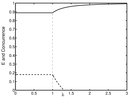
Figure 1: Concurrence (dashed line) and genuine tripartite entanglement $E$ (solid line) of the ground state of the isotropic spin-$\frac{1}{2}XY$ chain with three-spin interaction vs $\lambda$. The second-order quantum phase transition is signaled at $\lambda=1$ by both entanglement measures, but the singularity at $\lambda=2/(\sqrt{2}-1)\pi$ shown by the concurrence does not correspond to a quantum phase transition.

As an application, we consider the connection between the genuine tripartite entanglement of the ground state and the quantum phase transition of the isotropic spin-$\frac{1}{2}XY$ chain with three-spin interaction presented in Refs. [17, 18], which is an exactly solvable quantum spin model. The Hamiltonian is

$$H = -\sum_{i=1}^{N}\left[\sigma_{i}^{x}\sigma_{i+1}^{x}+\sigma_{i}^{y}\sigma_{i+1}^{y}\right.$$ (27)

$$\left.+\frac{\lambda}{2}\left(\sigma_{i-1}^{x}\sigma_{i}^{z}\sigma_{i+1}^{y}-\sigma_{i-1}^{y}\sigma_{i}^{z}\sigma_{i+1}^{x}\right)\right],$$

where $N$ is the number of sites, $\sigma_{i}^{\alpha}$($\alpha=x,y,z$) are the Pauli matrices, and $\lambda$ is a dimensionless parameter characterizing the three-spin interaction strength. Here the periodic boundary condition $\sigma_{N+1}=\sigma_{1}$ is assumed. The ground state of the spin-$\frac{1}{2}XY$ chain can always be considered as a tripartite $\left(2\otimes 2\otimes\left[2N-4\right]\right)-$dimensional pure state by a grouping such as two-nearest-neighbor-particle vs. others. One can safely employ $E$ to measure the genuine tripartite entanglement. The two-nearest-neighbor-particle density matrix can be given [18] by

$$\rho_{i,i+1}=\left(\begin{array}[]{cccc}\frac{(1-G^{2})}{4}&0&0&0\\ 0&\frac{(1+G^{2})}{4}&\frac{G}{2}&0\\ 0&\frac{G}{2}&\frac{(1+G^{2})}{4}&0\\ 0&0&0&\frac{(1-G^{2})}{4}\end{array}\right)$$ (28)

in the standard basis {$\left|\uparrow\uparrow\right\rangle,\left|\uparrow\downarrow\right\rangle,\left|\downarrow\uparrow\right\rangle,\left|\downarrow\downarrow\right\rangle$}, where

$$G=\left\{\begin{array}[]{cc}\frac{2}{\pi},&\lambda<1,\\ \frac{2}{\pi\lambda},&\lambda\geq 1.\end{array}\right.$$ (29)

Using eq. (4), one can easily calculate the genuine tripartite entanglement shown in Fig. 1. It is obvious that the first derivative of $E$ is discontinuous at $\lambda=1$ which consistent with Ref. [17] shows that the three-spin interaction leads to a second-order quantum phase transition. $E$ and its first derivative do not show any other singularity, which implies that $E$ faithfully signals a quantum phase transition. But the first derivative of the ground-state concurrence of two nearest-neighbor spins yields another discontinuity at $\lambda=2/(\sqrt{2}-1)\pi$ shown in Fig. 1, implying that the concurrence is misleading for this model.

IV Discussion and conclusion

We have introduced an entanglement monotone to measure the genuine tripartite entanglement existing in a given tripartite $(2\otimes 2\otimes n)-$dimensional quantum pure states in terms of a new bipartite entanglement measure. It is a new method to characterize genuine tripartite entanglement because it collects the contribution of all GHZ-type entanglement. Furthermore, it is interesting that the squared genuine tripartite entanglement monotone is the same as the original residual entanglement [9] for $(2\otimes 2\otimes 2)-$dimensional systems. The extension to mixed states (including the bipartite entanglement monotone) is straightforward in principle based on the convex roof construction [19], but an operational lower bound seems to be a bit difficult which is left to our forthcoming works. As an application, we considered the genuine tripartite entanglement of the ground state of the exactly solvable isotropic spin-$\frac{1}{2}$ chain with three-spin interaction. It is shown that the singularity of the genuine tripartite entanglement exactly signals a quantum phase transition. However, we only considered the given grouping method. The other $2\otimes 2\otimes 2\left[N-2\right]$ groupings can also be considered. Then, the tripartite entanglement monotone may be further employed to analytically study the quantum phase transition of more physical systems.

V Acknowledgement

This work was supported by the National Natural Science Foundation of China, under Grant No. 10747112, No. 10575017 and No. 10774020.

References

• (1) W. K. Wootters, Phys. Rev. Lett. 80, 2245 (1998).
• (2) A.Uhlmann, Phys. Rev. A 62, 032307 (2000).
• (3) K. Audenaert, F.Verstraete and De Moor, Phys. Rev. A 64, 052304 (2001).
• (4) Valerie Coffman, Joydip Kundu, and William K. Wootters, Phys. Rev. A 61, 052306 (2000).
• (5) W. Dรผr, G. Vidal, and J. I. Cirac, Phys. Rev. A 62, 062314 (2000).
• (6) A. Miyake, Phys. Rev. A 67, 012108 (2003).
• (7) Andreas Osterloh, Jens Siewert, Phys. Rev. A 72, 012337 (2005).
• (8) A. Miyake, F. Verstraete, Phys. Rev. A 69, 012101 (2004).
• (9) Alexander Wong and Nelson Christensen, Phys. Rev. A 63, 044301 (2001).
• (10) Chang-shui Yu, He-shan Song, Phys. Rev. A 72, 022333 (2005).
• (11) Chang-shui Yu, He-shan Song, Phys. Rev. A 73, 032322 (2006).
• (12) Chang-shui Yu, Ya-hong Wang, He-shan Song, Quantum Information and Computation 7(7), 584 (2007).
• (13) A. R. R. Carvalho, F. Mintert, A. Buchleitner, Phys. Rev. Lett. 93, 230501 (2004);
• (14) Chang-shui Yu, He-shan Song, Phys. Rev. A 73, 022325 (2006).
• (15) D. A. Meyer and N. R. Wallach, J. Math. Phys. 43, 4273 (2002).
• (16) G. K. Brennen, Quant. Inf. Comp. 3, 619 (2003).
• (17) P. Lou, W. C. Wu, and M. C. Chang, Phys. Rev. B 70, 064405 (2004).
• (18) M. F. Yang, Phys. Rev. A 71, 030302(R) (2005).
• (19) M.B. Plenio and S. Virmani, Quantum Information and Computation 7(1&2), 1 (2007).