Discovery of Spatial Periodicities in a Coronal Loop using Automated Edge-Tracking Algorithms

Abstract

A new method for automated coronal loop tracking, in both spatial and temporal domains, is presented. Applying this technique to trace data, obtained using the 171Å filter on 1998 July 14, we detect a coronal loop undergoing a 270 s kink-mode oscillation, as previously found by Aschwanden et al. Asc99 (1999). However, we also detect flare-induced, and previously unnoticed, spatial periodicities on a scale of 3500 km, which occur along the coronal-loop edge. Furthermore, we establish a reduction in oscillatory power for these spatial periodicities of 45% over a 222 s interval. We relate the reduction in detected oscillatory power to the physical damping of these loop-top oscillations.

1. Introduction

Automated feature recognition and tracking has long been a goal for scientists. With the advent of higher sensitivity satellite-based telescopes and the resulting increase in readout rates, it is imperative to be able to do some preliminary data analysis in real time. Without this ability, the large data rates achievable make it extremely difficult to implement onboard trigger programmes (e.g. a flare trigger) which allow the telescope pointing to be redirected to an area of interest almost immediately. Furthermore, having a means of establishing solar phenomena in real time allows instrument users to select datasets of particular interest much more readily than in the past. Thus, many schemes have been set up to push this form of real-time data analysis forward, including the Heliophysics Knowledge Base programme, which will enable real-time detections of oscillatory phenomena occurring on the Sun.

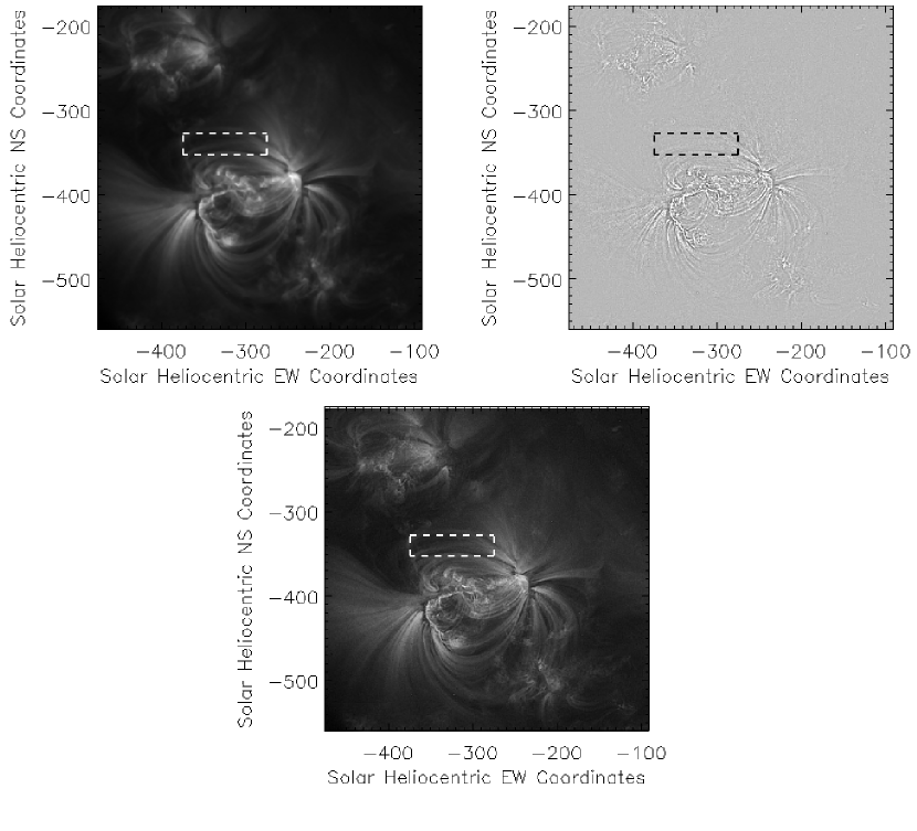
Figure 1.— Complete trace field of view (top left) after undergoing initial processing using the trace_prep.pro idl routine. The top right image shows the fine-scale structures detected using the Laplacian filter outlined in § 3.1 and the bottom image reveals the sharpened trace field of view after the addition of fine-scale structures. Note how the clarity of loop structures is drastically increased. Overplotted dashed lines in each image outlines the region of interest selected for this paper.

Current satellites, in particular the Transition Region And Coronal Explorer, trace, have enabled the analysis of many oscillatory signatures originating within the outer solar atmosphere. Aschwanden et al. Asc99 (1999), Schrijver et al. Sch02 (2002), Wang & Solanki Wan04 (2004), De Pontieu et al. Dep05 (2005) and Marsh & Walsh Mar06 (2006), just to name a few typical examples (a recent review is in e.g. Banerjee et al. 2007), all report oscillatory phenomena occurring within coronal loop structures. Previously, however, the majority of work on oscillating coronal loops has been focused on the temporal domain (e.g., Nakariakov et al. 1999). However, it was suggested by Erdélyi & Verth erd07 (2007) and Verth et al. ver07 (2007) that the imaging capacities of current and future high-resolution instruments should allow us to investigate oscillatory phenomena in the spatial domain (e.g. along the observed waveguide). Inspired by these suggestions, in this work we investigate the spatial evolution of a coronal loop structure, independent of its position during a flare-induced kink oscillation. From this we can understand the behaviour of the loop, in the spatial domain, and analyse any phenomena which are flare induced, yet confined to the volume occupied by the loop. In § 2 we describe the observations, while in § 3 we discuss the methodologies used during the analysis of the data which allow us to accurately track the spatial evolution of coronal loops. A discussion of our results in the context of confined loop oscillations is given in § 4, and our concluding remarks are in § 5.

2. Observations

The data presented here are part of an observing sequence obtained on 1998 July 14, using the trace imaging satellite. The optical setup of trace allowed a $384\arcsec~{}\times~{}384\arcsec$ area surrounding active region NOAA 8270 to be investigated with a spatial sampling of $0.5\arcsec$ per pixel. The 171Å filter was selected for these observations, which has an inherent passband width of 6.4Å, allowing plasma in the temperature range 0.2–2.0 MK to be studied. The cadence of the trace instrument was not constant during the observing sequence, with the time between successive exposures varying between 66 and 82 s.

Our dataset consists of 88 successive trace images providing nearly two hours of continuous, uninterrupted data. During the observing sequence, a large M4.6 flare occurred in the immediate vicinity of the active region under investigation.

3. Data Analysis

The trace data was retrieved directly from the Lockheed Martin Solar and Astrophysics Labs database and was subjected to standard processing algorithms: The idl routine trace_prep.pro was implemented to remove cosmic-ray streaks, reduce readout noise and prepare the data in a user-friendly format. De-rotation of the trace images was also deemed necessary, since the observing sequence lasts approximately two hours, equating to a relatively large solar rotation ($20\arcsec$ at disk centre). From this point, it was possible to use additional programmes to aid in the analysis of the data as described in detail below.

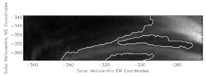
Figure 2.— A contoured (bold white line) trace coronal loop using a minimum intensity threshold of the background median value plus 5 sigma. From this threshold value we can see that the loop is contoured accurately with minimal solar background included.

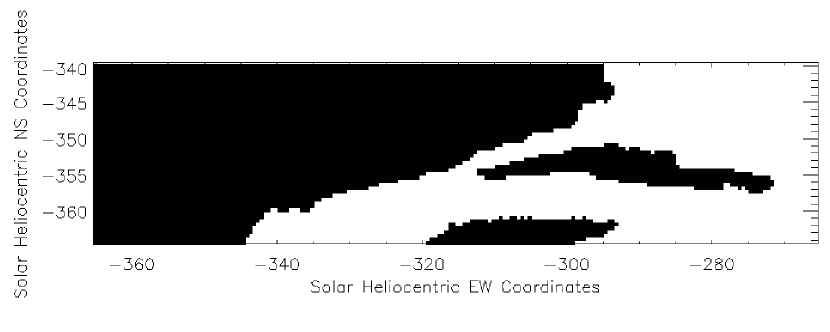
Figure 3.— The contours obtained in Figure 2 are converted to a binary scale as defined in § 3.2. This provides the sharp intensity gradient required for accurate feature edge detection and tracking.

3.1. Laplacian Image Sharpening

We implement a form of Laplacian image sharpening. Using the same 3-by-3 convolution kernel implemented by Gonzalez & Woods Gon92 (1992), we are able to enhance the fine-scale structure found in the trace images. Figure 1 shows the result of applying the convolution kernel to a full trace image. Note the amount of fine detail found in this filtered image (top-right panel of Fig 1). The next step is to add this fine-scale information back into the original image in order to sharpen the image. Note, in the bottom panel of Figure 1, the emphasis of fine structures when compared to the original, unfiltered image. Figure 1 demonstrates that these processes are readily applicable to full-size trace fields of view due to the fast processing ability of modern day computers. For the purposes of the data under investigation here, all trace images were subjected to Laplacian image sharpening routines.

3.2. Wavelet Modulous Maxima Edge Detection

After successful completion of image sharpening, edge detection algorithms can be implemented. The sharpened images have increased fine-scale information and as such provide the necessary platform for establishing feature edges which may have been previously unresolvable. Immediately after the flare event, one particular coronal loop is seen to oscillate. This kink-mode oscillation has been investigated many times (see Aschwanden et al. 1999 for the initial investigation) in the temporal domain. However, following Erdélyi & Verth erd07 (2007), we propose here to investigate the behaviour of the loop in the spatial domain. In order to track the spatial behaviour of the loop, an automated routine was devised to minimise errors introduced through human interaction with the data.

The first step involves intensity thresholding, whereby features in the trace field-of-view are contoured depending on their emissive flux. Threshold limits for contouring are entirely arbitrary and as such may vary from dataset to dataset as well as for which features are desirable to contour. However, for the data presented here, a lower intensity threshold of the background median value plus 5 sigma is used. This value allowed us to contour trace coronal loop structures, yet leave out background quiet Sun as shown in Figure 2. To emphasize feature edges and remove shallow intensity gradients, a binary format for feature mapping is used. All pixels which lie above the lower intensity threshold defined above are assigned a value of ‘1’. Those pixels which lie below the threshold were assigned a value of ‘0’, as seen in Figure 3. This binary format provides an absolute intensity cut-off thus providing a definite feature edge which can be tracked, both spatially and temporally. Placing the images into binary format was deemed necessary due to the poor spatial resolution of the trace spacecraft, whereby neighbouring bright features are hard to distinguish unless a form of thresholding is used. Future instruments, which provide higher spatial resolution, should eradicate the need for binary formatting. The binary image is padded using a zeroed array from which feature edge tracking can commence.

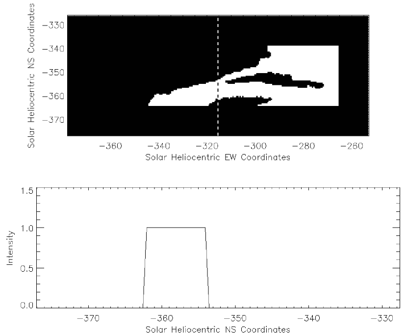
Figure 4.— Upper panel shows the binary-formatted image obtained in Figure 3 inserted into a padded, zeroed array which provides the best platform for WMM edge detection. A vertical dashed line at x pixel 125, corresponding to a Heliocentric E/W coordinate of -315^′′, is drawn, with the resulting intensity plot, along the N/S direction for this x pixel, shown in the bottom panel.

Tracking of this feature edge is performed using a Wavelet Modulous Maxima (WMM) technique (Muzy et al. 1993, McAteer et al. 2007). From the padded binary array created above, a horizontal pixel is chosen. Figure 4 shows the selection of horizontal pixel 125, as indicated by the vertical dashed line, as well as the corresponding intensity plot along this vertical line. A wavelet transform is produced for this intensity plot, demonstrated in Figure 4, utilizing a Mexican Hat wavelet. A Mexican Hat wavelet, which is a double derivative of the traditional Morlet wavelet, is very useful for detecting sharp intensity gradients which are present due to the binary format implemented above. An absolute wavelet power spectrum is plotted as a function of vertical pixel element in Figure 5. Additionally, maximum wavelet power features are traced down to the x-axis of the power spectrum and reveal the locations of maximum intensity gradients. Figure 5 re-plots the intensity in the vertical direction at horizontal pixel 125 and it can be seen that where the maximum wavelet power meets the x-axis also corresponds to the edges of the trace coronal loop under investigation.

From Figure 2, it is clear that better contrast is achieved at the Northern edge of the loop where its brightness overlies fainter, less intense, quiet Sun. By contrast, the Southern edge of the loop in Figure 2 is difficult to separate from other loop structures, due to the densely packed nature of such features closer to active regions. Since in this instance it is desirable to track the upper edge of the coronal loop, we disregard the first maximum wavelet power location and record the position where the second maximum wavelet power location intersects with the x-axis. This pin points the exact location of the Northerly edge of the coronal loop in question. This process is repeated over the entire E/W direction, and for all frames in the observing sequence, with the subsequent position of the Northern edge of the trace coronal loop recorded. From the resulting loop edge positions, it is possible to analyse both temporal, and spatial, variations.

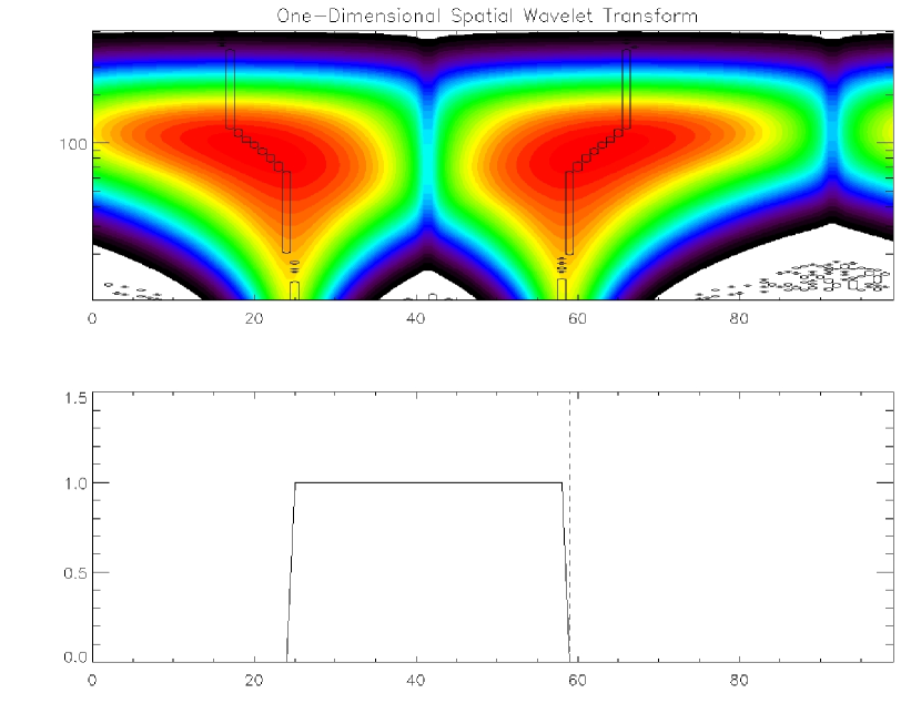
Figure 5.— The wavelet power spectrum (top) generated along the vertical spatial direction of the trace field of view for horizontal pixel number 125. This panel also shows regions of maximum power being traced down to the intersect point on the x-axis. The intensity plot from Figure 4 is again plotted (bottom) with a dashed line indicating the position of intersection of the maximum wavelet power traces with the x-axis. Notice how the x-axis intersect position of maximum wavelet power corresponds exactly to the reduction of intensity in the bottom panel. This reduction in intensity is analagous with the upper edge of the trace coronal loop showing the accuracy of this method when detecting feature edges.

4. Results and Discussion

Our main goal is to investigate the spatial behaviour of the oscillating coronal loop. However, to verify that the presented loop-tracking routine is functioning properly, derived results in the temporal domain are compared to previous findings. To compensate for the timing irregularity outlined in § 2, all data were interpolated onto a constant-cadence time series with linear interpolation performed between data points. This provides the necessary platform for temporal studies to commence. Maintaining consistency with the previous example, a plot indicating the variation with time of the location of the Northern edge of the coronal loop, for horizontal pixel 125, is displayed in Figure 6. It is clear that a periodicity of approximately 270 s exists, consistent with the findings of Aschwanden et al. Asc99 (1999). This result implies that the loop detection and tracking algorithms, developed here, are functioning accurately.

From Figure 6, it appears that the oscillating coronal loop passes through an equilibrium position at times of 0, 280 and 502 s, with the overall shape of the loop similar at the corresponding trace frames. If indeed the shape of the loop is identical at times of 0, 280 and 502 s, then a subtraction of any two of these loop shapes should provide a resulting image equal to zero. However, upon subtraction of the loop shape at 0 s from that at 280 s, a spatial periodicity is revealed. Running this resulting loop shape through a one-dimensional spatial wavelet transform establishes an oscillatory period along the Northern loop edge of 10 pixels (Fig 7). A number of strict criteria implemented on the data, including the test against spurious detections of power that may be due to Poisson noise, the comparison of the input lightcurve with a large number (1500) of randomized time-series with an identical distribution of counts (see O’Shea et al. 2001 for a detailed explanation) and the exclusion of oscillations which last, in duration, less than $1.41$ cycles, allowed us to insure that oscillatory signatures correspond to real periodicities. These criteria have been described in detail in previous papers (see Jess et al. 2007, Banerjee et al. 2001, McAteer et al. 2004, Ireland et al. 1999, Mathioudakis et al. 2003). Furthermore, according to the Ritz theorem of variational principles (Ritz 1908), spatial amplitude dependence is much more sensitive to structural changes of the magnetic loop (e.g. stratification, magnetic field divergence, twist etc.) than the traditionally studied period ratios of FFT-identified modes of oscillations. Thus, analysing spatial variations, rather than the more traditional temporal variations, will provide a useful platform in which to maximize the limited resolution of current satellite imagers. For the trace plate scale equal to $0.5\arcsec$ per pixel, the detected 10 pixel periodicity corresponds to an absolute spatial distance, or wavelength, of approximately 3500 km per complete oscillation (more than three complete cycles detected).

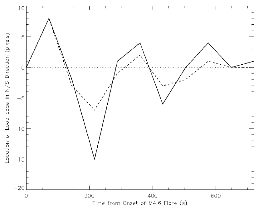
Figure 6.— The temporal evolution of a particular portion of the oscillating coronal loop. Here, shown as a bold line, we see a periodicity of approximately 270 s related to the kink-mode oscillation of the loop and the subsequent damping of the amplitude with time. The dashed line indicates the temporal periodicity detected when a lower-intensity threshold is used to contour the loop edge, while the dotted line indicates the equilibrium position of the loop. A lower intensity threshold (see § 4) reveals the same periodicity, indicating that the loop-edge tracking, due to high contrast between the loop and surrounding quiet sun, is not overly sensitive to threshold values.

To investigate if this periodicity is visible at the following equilibrium position (502 s), we subtract the loop shape at 0 s from that at 502 s, and pass through our one-dimensional spatial wavelet transform. The resulting evidence, shown in Figure 8, indicates that the 10 pixel spatial periodicity is indeed still present, albeit with a reduction in oscillatory power. We interpret the reduction in oscillatory power as the physical signature of damping of the loop-top oscillations. On further inspection of Figures 7 and 8, we see that the oscillatory power, in normalised digital number (DN), has dropped from 29 to 16 over the 222 s interval. This equates to a 45% decrease in oscillatory power and is consistent with other aspects of coronal-loop oscillations, which are seen to be heavily damped (Aschwanden et al. 2003, Ruderman 2005, Terradas et al. 2006, Dymova & Ruderman 2007).

To investigate a possible phase relationship (Athay & White 1978, O’Shea et al. 2007), we create a cross-wavelet power spectrum between the two detected loop-top oscillations, and inspect the resulting spatial-phase diagram (Fig 9). This figure reveals a clear phase shift, over many complete wavelengths, of $0^{\circ}$ to $-50^{\circ}$. Due to the long kink-oscillation period ($\approx$ 270 s), and the relatively poor, and irregular, cadence of the trace instrument, we are only able to evaluate kink-equilibrium spatial periodicities at two times during the presented dataset. At these two times, the coronal loop undergoing the kink oscillation has returned to it’s equilibrium state - i.e. matching the shape and position of the loop prior to the flare-induced kink oscillation. Between these two equilibrium states, the loop in question has undergone one complete kink-oscillation cycle.

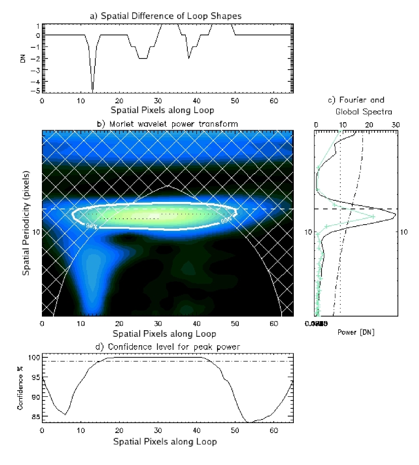
Figure 7.— The detection of a 10 pixel spatial oscillation. The resulting Northern loop-edge outline created by the subtraction of the loop edge at 0 s from the loop edge at 280 s after the flare event is shown in a). The one-dimensional spatial wavelet power transform along with locations where detected power is at, or above, the 99% confidence level are contained within the contours in b). Plot c) shows the summation of the wavelet power transform over time (full line) and the Fast Fourier power spectrum (crosses) over time, plotted as a function of period. Both methods have detected a well pronounced 10 pixel spatial oscillation. The global wavelet (dashed dotted line) and Fourier (dotted line) 95% significance levels are also plotted. The cone of influence (COI), cross-hatched area in the plot, defines an area in the wavelet diagram where edge effects become important and as such any frequencies outside the COI are disregarded. Periods above the horizontal line (dotted) fall within the COI. The probability levels, which are related to the percentage confidence attributed to the peak power at every time step in the wavelet transform, are plotted in d).

However, since we cannot evaluate more than two kink-equilibrium spatial periodicities, we are unable to determine the direction of wave propagation. Three or more kink-equilibrium positions would allow for a comparison of phase differences, thus providing an indication to the direction of wave propagation. Thus, a phase shift of $0^{\circ}$ to $-50^{\circ}$ may equally be represented as $(n360)^{\circ}$ to $(n360-50)^{\circ}$, where $n$ is an integer number arising from the low sampling rate of the trace instrument. As described by Athay & White Ath79 (1979) and O’Shea et al. Osh06 (2006), the errors associated with the phase shift can only be constrained and determined unambiguously by careful measurements over the full range of observed wavelengths. To reduce the errors involved with phase difference analysis we evaluate the phase shift over a number of different wavelengths. Through examination of the Fourier and global spectra associated with the detected 3500 km spatial oscillation, in addition to the boundaries of the 99% confidence-level contours, we find that the FWHM of the presented oscillation is 5 pixels, or $\approx$ 1800 km. This corresponds to 42 wavelength resolution elements, when using a 0.016 spacing between discrete scales, in the evaluation of the cross-wavelet power spectrum (Torrence & Compo 1998). Performing phase difference analysis on each of the 42 wavelength elements, spanning a wavelength coverage of 2600–4400 km, we are able to verify the existence of a $0^{\circ}$ to $-50^{\circ}$ phase shift. More importantly, we can reduce the error associated with the calculated phase differences through examination of the multiple wavelength elements. The bottom panel of Figure 9 includes the maximum deviation, from the average spatial-phase diagram, induced by the analyses of 42 wavelength resolution elements. It can be seen from Figure 9 that the phase error bars do not detract from the generalized shape of the spatial-phase diagram, thus validating the existence of a $0^{\circ}$ to $-50^{\circ}$ phase shift.

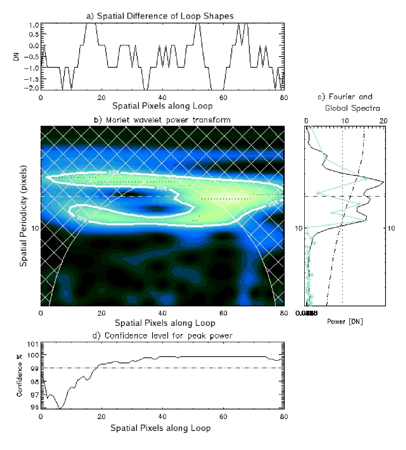
Figure 8.— Identical plot to Figure 7, except the loop-edge outline shown in a) results from the subtraction of the loop edge at 0 s from the loop edge at 502 s after the flare event. We can see that a 10 pixel spatial periodicity is still evident, albeit with a reduction in normalised oscillatory power.

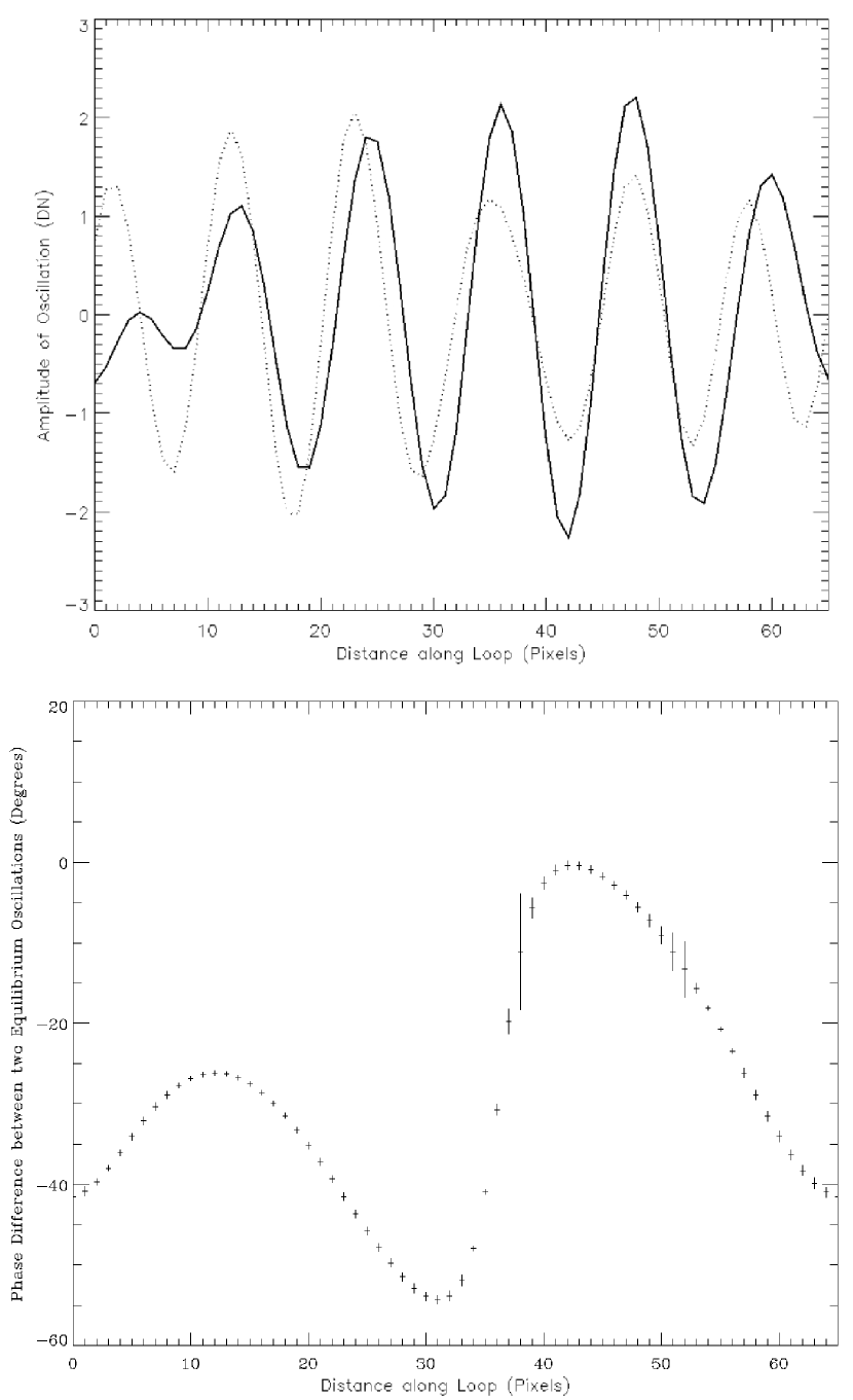
Figure 9.— The top panel shows the oscillation amplitude as a function of position along the loop for both loop-top oscillations. The solid line relates to the spatial periodicity detected between times of 0 and 280 s, while the dotted line relates to the spatial periodicity detected between times of 0 and 502 s. From this plot, it is clear to see a phase shift between the two loop-top oscillations. The bottom panel shows the phase-difference results of a cross-wavelet spectrum of the two detected spatial oscillations. Maximum phase deviations from the average spatial-phase curve, as detailed in § 4, are plotted as vertical error bars. We can clearly see a phase shift, on the order of $0^{\circ}$ to $-50^{\circ}$, over the duration of 6 complete cycles.

In order to validate our results, we have undertaken a number of further rigorous tests. We have implemented the same loop-edge detection and tracking processes on additional coronal loops away from the region under investigation, yet within the same trace field of view. Since these loops are not connected with the flare event, and therefore not seen to oscillate, no spatial periodicities along the loop would be expected when two loop outlines are subtracted from one and other. Subtracting the control loop outline at 0 s from that at 280 s after the flare, to remain consistent with the work above, and running through a one-dimensional spatial wavelet transform reveals no periodicities. Furthermore, we tested for spatial periodicities, on the loop seen to oscillate, both prior to, and long after, the flare event. These tests found no oscillatory phenomena in either instance, indicating that the spatial periodicities detected are flare induced. To further test the abilities of the presented algorithm, we carry out an identical form of analysis on an additional case of an oscillating coronal loop observed by trace on 2001 April 15. We chose a loop arcade which is seen to oscillate after being buffeted by a neighbouring X14.4 flare originating from NOAA 9415. Implementing our algorithm on this dataset we are able to corraborate the kink periodicity and associated decay time described by Verwichte et al. Ver04 (2004). However, in this instance no coronal-loop spatial periodicities could be found. The presented algorithm is therefore applicable to all datasets and is a reliable tool for detecting kink oscillations.

Additionally, to verify that the detected oscillation is not an artifact of the loop-tracking algorithm, we have designed a numerical simulation to test the reliability of our oscillatory signal. A synthetic wave train is generated which is identical in both amplitude and wavelength to the detected trace oscillations, and propagates with an Alfvén speed of 1000 km/s (Nakariakov & Verwichte 2005). A resultant wave, formed from the numerical integration with time, is created based on real exposure times extracted from the trace image files. As would be expected, if the exposure time is an exact integer multiple of the oscillatory period, the resultant wave form equals zero at all spatial locations (Fig 10). This is due to,

$$\int_{0}^{n2\pi}\mathrm{Sin(}t\mathrm{)~{}d}t=0$$ (1)

where $n$ is an integer number and $t$ is time. By contrast, if the exposure time is set to a value not equal to an integer multiple of the period, then the propagating wave can be detected. Figure 11 shows the resultant wave, formed using the exact exposure time taken from the trace images. It is clear, from Figure 11, that even though multiple oscillatory cycles pass through the same pixel on the detector, an oscillatory periodicity can still be detected.

Throughout the analysis of the presented results, we interpret the translation of the coronal loop, both in the temporal and spatial domains, to be the result of the physical movement of this feature. Other aspects may accompany, and subsequently aid, in the movement of the loop. Things such as a change in temperature, or a change in inclination angle, may result in line-of-sight intensity changes. Since the trace bandpass used allows a wide range of coronal temperatures to be investigated, and since the movement of the loop edge is restricted to $<10^{\prime\prime}$, we feel confident that the main source of translation is caused by the physical movement of the loop itself.

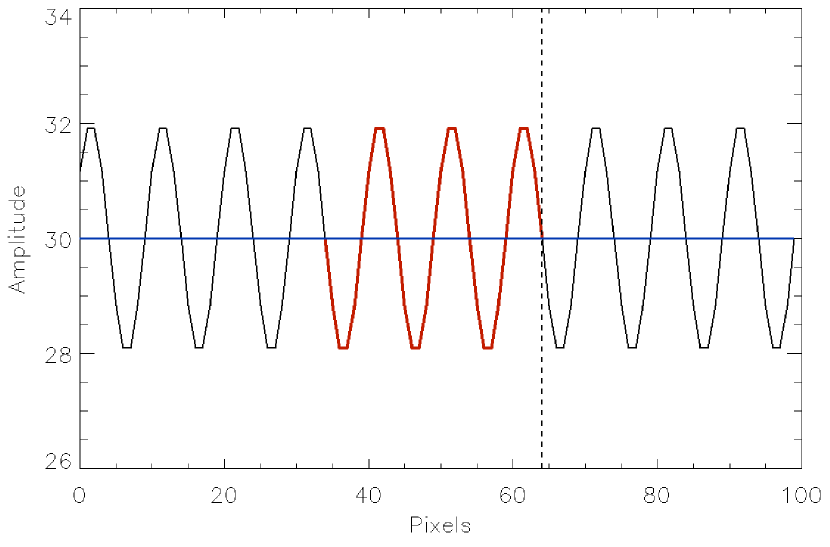
Figure 10.— The integrated wave form when the exposure time is equal to an integer number of complete periods. The black wave train is a sinusoid, equal in both amplitude and wavelength, to the observed trace spatial oscillation. The bold red line indicates the portion, of the input wave train, which passes through an arbitrary spatial location, as denoted by the vertical black dashed line, during the exposure time. The result of integrating over the chosen exposure time is plotted as a bold blue line. It is clear that the resultant wave, when the exposure time is equal to an integer multiple of the period, equals zero. This wave will therefore not be detectable by the trace instrument.

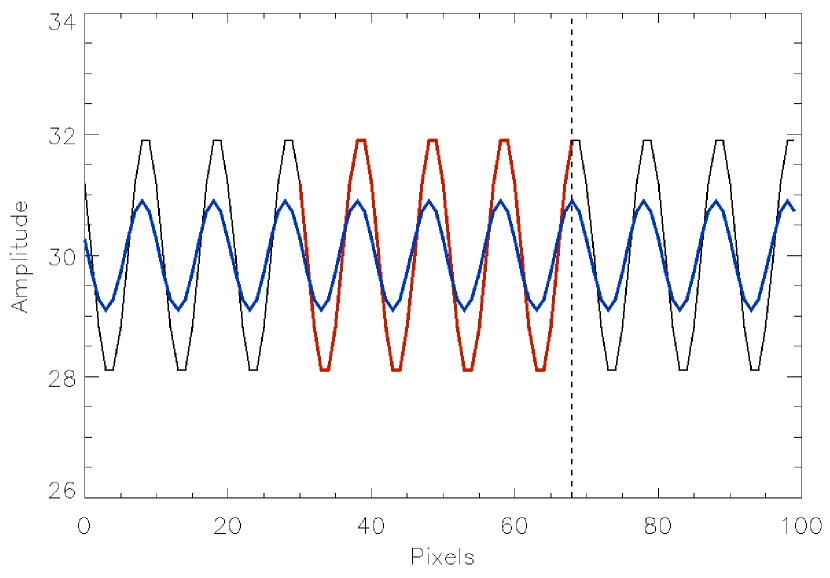
Figure 11.— Identical plot to Figure 10, only showing the resultant wave form produced when the exposure time matches that of the trace instrument. It is clear that the resultant wave, unmodified in wavelength, is still detectable even when multiple oscillations pass through the same pixel on the detector. This plot demonstrates that our detected 3500 km spatial periodicity is real.

5. Concluding Remarks

A new method for the detection, and subsequent tracking, of coronal loop structures is presented. This method also provides the ability to simultaneously search for longitudinal and transverse oscillations in real-time. It is possible to detect the periodic loop displacement caused by the influence of transverse waves, and in addition the intensity fluctuations, due to density restrictions and rarefactions, synonymous with longitudinal oscillations can also be easily identified through concurrent time-series analysis. Through the subtraction of loop outlines, we are essentially removing general features and shapes which remain constant from frame to frame, yet magnifying features which evolve or change spatial position. Utilizing our method for automated coronal loop analysis, we have detected spatial periodicities, on the scale of 3500 km per cycle, occurring on a coronal loop immediately after being buffeted by a neighbouring M4.6 flare. We detect the damping of these loop-top oscillations, with a 45% reduction in oscillatory power over a 222 s interval. In addition, we find a wrapped spatial phase shift of $0^{\circ}$ to $-50^{\circ}$, related to the time interval of 222 s between successive kink-oscillation equilibrium positions, for the travelling loop-top oscillations.

We propose the above methodology will be useful in the future, especially with both temporal and spatial resolutions of space-borne solar telescopes constantly improving. From coronal imagers available on the upcoming Solar Dynamics Observatory and Solar Orbiter, as well as the recently launched Hinode satellite, there will be a wealth of high-resolution images containing abundances of coronal loop oscillations. There are a number of currently available methods to detect and analysis such oscillatory phenomena. Such techniques may be data specific, and therefore not applicable to a wide range of varying coronal observations. However, our technique is designed to be readily applicable to all coronal datasets, and is a great asset when spatial resolutions are of the highest order due to the WTMM techniques outlined here. We suggest that the currently presented method provide further excellent capabilities for the detection of both temporal and spatial coronal loop oscillations.

References

- (1) Aschwanden, M. J., Fletcher, L., Schrijver, C. J., & Alexander, D., 1999, ApJ, 520, 880–894
- (2) Aschwanden, M. J., Nightingale, R. W., Andries, J., Goossens, M., & Van Doorsselaere, T., 2003, ApJ, 598, 1375–1386
- (3) Athay, R. G., & White, O. R., 1978, ApJ, 226, 1135
- (4) Athay, R. G., & White, O. R., 1979, ApJ, 229, 1147
- (5) Banerjee, D., Erdélyi, R., Oliver, R. & O’Shea, E., 2007, Solar Phys., in press
- (6) Banerjee, D., O’Shea, E., Doyle, J. G., & Goossens, M., 2001, A&A, 371, 1137
- (7) De Pontieu, B., Erdélyi, R. & De Moortel, I., 2005, ApJ, 624, L61
- (8) Dymova, M. V., & Ruderman, M. S., 2007, A&A, 463, 759
- (9) Erdélyi, R. & Verth, G., 2007, A&A, 642, 743
- (10) Gonzalez, R., & Woods, R., 1992, Digital Image Processing, Addison Wesley, 414–428
- (11) Ireland, J., Walsh, R. W., Harrison, R. A., & Priest, E. R., 1999, A&A, 347, 355
- (12) Jess, D. B., Andic, A., Mathioudakis, M., Bloomfield, D. S., & Keenan, F. P., 2007, A&A, 473, 943
- (13) McAteer, R. T. J., Gallagher, P. T., Bloomfield, D.S., Williams, D. R., Mathioudakis, M., & Keenan, F.P., 2004, ApJ, 602, 436–445
- (14) McAteer, R. T. J., Young, C. A., Ireland, J., & Gallagher, P. T., 2007, ApJ, 662, 691–700
- (15) McEwan, M. P., & De Moortel, I., 2006, A&A, 448, 763–770
- (16) Marsh, M. S., & Walsh, R. W., 2006, ApJ, 643, 540–548
- (17) Mathioudakis, M., Seiradakis, J. H., Williams, D. R., Avgoloupis, S., Bloomfield, D. S., & McAteer, R. T. J., 2003, A&A, 403, 1101–1104
- (18) Muzy, J. F., Bacry, E., & Arneodo, A., 1993, Phys. Rev., E-47, 875–884
- (19) Nakariakov, V. M., Ofman, L., Deluca, E. E., Roberts, B., Davila, J. M., 1999, Science, 285, 862–864
- (20) Nakariakov, V. M., & Verwichte, E., 2005, LRSP, 3
- (21) O’Shea, E., 2001, A&A, 368, 1095
- (22) O’Shea, E., Banerjee, D., & Doyle, J. G., 2006, A&A, 452, 1059–1068
- (23) O’Shea, E., Banerjee, D., & Doyle, J. G., 2007, A&A, 463, 713–725
- (24) Ritz, W., 1908, J. Reine Angew. Math., 135, 1–61
- (25) Ruderman, M. S., 2005, Proc. Dynamic Sun : Challenges for Theory and Observations, ESASP-600, 96
- (26) Schrijver, C. J., Aschwanden, M. J., & Title, A. M., 2002, Sol. Phys., 206, 69–98
- (27) Sheeley, N. R., Wang, Y. M., Hawley, S. H., Brueckner, G. E., Dere, K. P., et. al., 1997, ApJ, 484, 472–478
- (28) Terradas, J., Oliver, R., & Ballester, J. L., 2006, ApJ, 650, 91–94
- (29) Torrence, C., & Compo, G. P., 1998, Bull. Amer. Meteor. Soc., 79, 61
- (30) Verth, G., van Doorsselaere, T., Erdélyi, R. & Goossens, M. 2007, A&A, in press
- (31) Verwichte, E., Nakariakov, V. M., Ofman, L., & DeLuca, E.E., 2004, Sol. Phys., 223, 77–94.
- (32) Wang, T. J., & Solanki, S. K., 2004, A&A, 421, 33–36