Classical Antiferromagnetism on Torquato-Stillinger Packings

Abstract

Torquato and Stillinger have constructed a new family of frustrated lattices by unusually high dilution of close packed structures while preserving structural stability. We show that an infinite subclass of these structures has an underlying topology that greatly simplifies determination of their magnetic phase structure for nearest neighbor antiferromagnetism interactions and $O(N)$ spins.

I Introduction

The face centered cubic lattice and its close packed relatives are interesting in two distinct contexts. The first is their structural stability as close packed structures Ashcroft and Mermin (1976). The second is their giving rise to geometrical frustration when they host magnetic degrees of freedom Anderson (1950); Luttinger (1951).

In a recent development, Torquato and Stillinger Torquato and Stillinger (2007) asked an intriguing question about these structures from the stability viewpoint: how many sites can you dilute from them without rendering them structurally unstable to shear forces? Their answer is a family of packings, which we shall term Torquato-Stillinger (TS) packings, with a local coordination number of 7 and a spherical packing density of $\frac{\sqrt{2}\pi}{9}$; for details we refer to Ref. Torquato and Stillinger, 2007.

In this paper we examine the TS packings from the viewpoint of geometrical frustration which survives the dilutions they envisage. Specifically we determine the ground states, low temperature ordering and the nature of the phase transition to the paramagnetic state in a large subclass of the TS packings for nearest neighbor antiferromagnetic interactions for classical Ising, XY, and Heisenberg spins and as well as for $O(N)$ spins with $N\geq 4$. In this task we will be greatly aided by the simple observation that this subclass of TS packings is topologically equivalent to a set of stacked triangular lattices with half of the stacking bonds removed. As stacked triangular lattices have been studied intensively (see Refs. Collins and Petrenko, 1997, Loison, 2005 and references therein), we will be able to carry over various results from that work.

In the following we first review the TS construction of their packings and single out a dilution of the FCC packing (lattice) as exemplifying the stacked triangular structure that we will focus on. Next we present results for antiferromagnetism on the TS-FCC packing and its relatives. We end with brief comments on the cases not studied in this paper.

II Lattices

General TS packings are constructed by removing one third of the sites from a close packing of spheres. To describe them more precisely recall first that any three dimensional close packing of spheres can be obtained by stacking two dimensionally close packed triangular lattices of spheres according to a prescribed stacking pattern. In a given triangular plane, the interior of triangular plaquettes host depressions into which further spheres may be placed. Of these we may select either all upward pointing triangles or all downward pointing triangles in which to place the spheres of the next triangular layer. The standard description labels the original sites as, say, C whereupon the two inequivalent depressions that host the second layer are labeled A and B. All layers consist of spheres occupying one of these three sets of sites with the rule that there is no repetition between adjacent layers—this gives rise to the $2^{N}$ Barlow packings for $N$ layers of spheres. As is well known, of these the repeated sequences ABC yield the FCC lattice and AB or AC yield the hcp structure Ashcroft and Mermin (1976).

An equivalent description can be given in terms of two stacking vectors which allow us to translate one triangular layer into a neighboring one. As they can be chosen independently at each step, we recover the previous counting. For concreteness, let us orient one of the triangular layers as shown in Fig. 1. Now the stacking vectors are readily seen to be

$${\bf V}_{\alpha} = -\frac{a}{2}\hat{\bf x}+\frac{\sqrt{3}a}{6}\hat{\bf y}+a\sqrt{\frac{2}{3}}\hat{\bf z}$$

$${\bf V}_{\beta} = \frac{\sqrt{3}a}{3}\hat{\bf y}+a\sqrt{\frac{2}{3}}\hat{\bf z}$$ (1)

where $a$ is the diameter of the spheres. Now, for example, the allowed configurations of three planes can be written as CAC (or ${\bf V}_{\alpha}$, ${\bf V}_{\beta}$), CBC (${\bf V}_{\beta}$, ${\bf V}_{\alpha}$), CAB (${\bf V}_{\alpha}$, ${\bf V}_{\alpha}$), CBA (${\bf V}_{\beta}$, ${\bf V}_{\beta}$).

Figure 1: The triangular lattice

To dilute a sphere packing into a TS packing, one vertex of each triangle in the triangular layers is removed, leaving stacked honeycomb layers. Now at each step there are 6 choices—a choice between two of the A, B, or C sites followed by a choice of which of the three equivalent sublattices of the triangular layer to dilute. All choices lead to stable structures Torquato and Stillinger (2007).

Equivalently, we may begin with one honeycomb layer and construct the rest of the structure by displacing it successively by stacking vectors drawn now from a set of six vectors. With our choice of orientation these are

$${\bf V}_{\beta 1} = \frac{a}{2}\hat{\bf x}-\frac{\sqrt{3}a}{6}\hat{\bf y}+a\sqrt{\frac{2}{3}}\hat{\bf z}$$

$${\bf V}_{\beta 2} = \frac{\sqrt{3}a}{3}\hat{\bf y}+a\sqrt{\frac{2}{3}}\hat{\bf z}$$

$${\bf V}_{\beta 3} = -\frac{a}{2}\hat{\bf x}-\frac{\sqrt{3}a}{6}\hat{\bf y}+a\sqrt{\frac{2}{3}}\hat{\bf z}$$

$${\bf V}_{\alpha 1} = -\frac{a}{2}\hat{\bf x}+\frac{\sqrt{3}a}{6}\hat{\bf y}+a\sqrt{\frac{2}{3}}$$

$${\bf V}_{\alpha 2} = -\frac{\sqrt{3}a}{3}\hat{\bf y}+a\sqrt{\frac{2}{3}}\hat{\bf z}$$

$${\bf V}_{\alpha 3} = \frac{a}{2}\hat{\bf x}+\frac{\sqrt{3}a}{6}\hat{\bf y}+a\sqrt{\frac{2}{3}}\hat{\bf z}$$

Now, starting as above with a C plane, ${\bf V}_{\alpha 1}$ through ${\bf V}_{\alpha 3}$ generate A planes, while ${\bf V}_{\beta 1}$ through ${\bf V}_{\beta 3}$ yield B planes. The projections of these vectors in the honeycomb planes are shown in Fig 2. Observe that the projections of the ${\bf V}_{\beta i}$ are inverses of the projections of the ${\bf V}_{\alpha i}$.

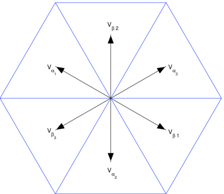
Figure 2: Projections of the 6 stacking vectors in the honeycomb planes. Note that all $V_{\alpha i}$ result in a CA stacking, and all $V_{\beta i}$ in a CB stacking.

Three comments are in order. First, the TS packings contain tunnels through the parent Barlow packings. The stacking vectors can also be visualized as giving the direction of the tunnels (in other words, the offset between the centers of the missing spheres in adjacent planes). Second, in the close packed case, irrespective of the stacking pattern, rotations by $2\pi/3$ radians about either the vertex or the center of a triangle are symmetries of the structure. After removing the centers of each hexagon, however, such rotations map some occupied sites to unoccupied sites and vice versa, breaking the symmetry. Third, all TS packings have a local coordination number of 7—3 nearest neighbors in a single honeycomb layer and 2 each in the layer above and below.

Clearly, there are $6^{N}$ TS packings for $N$ honeycomb layers. In this article we focus on a subset of them which is $2^{N}$ in number. We begin with one member of this subset which is defined by the single stacking vector ${\bf V}_{\beta 1}$. This particular choice known as the tunneled FCC lattice, is discussed extensively in Ref. Torquato and Stillinger, 2007; we will review its structure briefly here.

Written conventionally, this packing is a triclinic lattice with a two site unit cell. The primitive lattice vectors are

$${\bf a_{1}} = a(0,\sqrt{3},0)$$

$${\bf a_{2}} = a({3\over 2},-\frac{\sqrt{3}}{2},0)$$

$${\bf a_{3}} = a({1\over 2},-\frac{\sqrt{3}}{6},\sqrt{2\over 3})$$ (3)

The two atoms of the unit cell are at positions

$${\bf x}_{1} = a(0,0,0)$$

$${\bf x}_{2} = a(1,0,0)$$ (4)

The resulting lattice, shown in Fig. 3(a), consists of the honeycomb lattice in the $xy$ plane, with nearest neighbours separated by a distance $a$. The honeycomb layers are stacked in the $z$ direction according to the FCC pattern, with the same stacking vector ${\bf V}_{\beta 1}$ between every honeycomb plane.

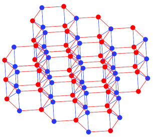
(a)

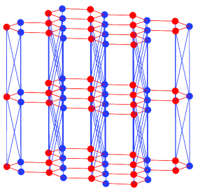
(b)

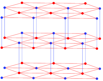
(c)

Figure 3: (a) The TS-FCC lattice as a set of stacked honeycomb lattices. Bonds in the honeycomb lattice ($xy$ plane) are colored red (dotted lines); bonds joining different honeycomb layers are blue (solid lines). The two colorings of the sites differentiate the 2 sublattices. (b) A rotated view that exhibits the alternate decomposition as a set of semi-stacked folded triangular planes. The planes are seen almost edge on and consist of sites from both sublattices. The lighter red (darker blue) sites are connected to dark blue (light red) sites in the folded triangular plane to the left (right). (c) The topologically equivalent stacked triangular lattice, with unfolded triangular planes now redrawn in the $xy$ plane.

We are primarily interested in nearest neighbor antiferromagnetism. For nearest neighbor interactions the TS-FCC lattice has an elegant reinterpretation that is extremely useful. As shown in Fig. 3(b) the honeycomb planes stack in such a way as to create folded sheets of stacked triangular lattices. The folded sheets run along two pairs of parallel edges in the hexagon. The remaining pair of edges bond neighbouring triangular sheets. This is made clear in Fig. 3(c) where we straighten out the triangular sheets and draw the topologically equivalent semi-stacked triangular lattice or SSTL. Unlike the case of the stacked triangular lattice (STL), in which each site has a nearest neighbour in the sheets above and below it, the stacking bonds in the SSTL alternately join sites in one sheet to the sheets above and below. The lattice co-ordination number is thus $7$ as it should be.

The TS-FCC lattice is one of an infinite subclass that share the same topology as the SSTL: any TS packing defined by stacking vectors that belong to one of the sets $\{{\bf V}_{\alpha i},{\bf V}_{\beta i}\}$ is equivalent to triangular sheets stacked in this way. Thus there are $3\cdot 2^{N}$ such packings for $N$ layers—up to the overall factor of $3$ for choice of sublattice diluted, this is the same as the number of the parent Barlow packings.

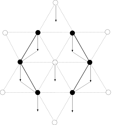
Figure 4: A schematic of the formation of triangular planes. One layer of the parent triangular lattice is shown, with black (white) circles representing occupied (vacant) sites. The arrows show the projection of the stacking vector $V_{\alpha 2}$ in the honeycomb plane. In a Barlow packing, the center of every upward facing triangle is an occupied site in the next layer, and the center of each triangle would be the apex of a tetrahedron. Both solid and dotted lines are nearest neighbour bonds for the Barlow packing. In the equivalent TS packing shown here, only the centers of the four triangles lying immediately below occupied sites are occupied in the next layer. The solid lines show nearest neighbour bonds in the TS packing. The darkened diagonal edges of the hexagon still form bases of triangles completed by the occupied sites in the next layer; the horizontal edges of the hexagon do not, and lie in the direction of stacking of the triangular sheets.

To see how this comes about, let us begin with stacking one plane above a reference plane with say ${\bf V}_{\alpha 2}$ and consider a given hexagon in the reference plane. Let us label the three sets of parallel bonds on the hexagon by the indices on the stacking vector projections orthogonal to them. As we see in Fig 4, two of the three sets of parallel bonds on the hexagon are now also bonds on triangles while one set—set 1—of parallel bonds is not. The same set is singled out when we use stacking vector ${\bf V}_{\beta 2}$ instead.

It follows then that if we use a sequence of ${\bf V}_{\alpha 2}$ and ${\bf V}_{\beta 2}$ to stack, we will get a sequence of honeycomb planes where the 2 and 3 bonds participate in triangles and it is easy to convince oneself that this will lead to the claimed topology. More precisely, the 2 and 3 bonds will lie in (folded) triangular planes connected by 1 (stacking) bonds. Conversely, if we decide to switch from the 1 stacking vectors to the 2 or 3 stacking vectors at some stage we will interfere with this topology. Hence the result.

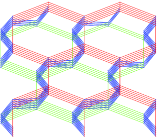
Figure 5: The TS-HCP lattice, showing stacking structure. Honeycomb planes are stacked according to an alternating ABAB pattern. The A planes are shown here in green (dotted lines), and the B planes in red (solid lines). In contrast to the TS-FCC case, the tunnels formed by vacant sites zig-zag between layers, giving the structure a 2 sublattice chirality Torquato and Stillinger (2007).

We have already discussed the TS-FCC lattice obtained by repeated stacking with the vector ${\bf V}_{\alpha 2}$. As another example we display, in Fig 5, the TS-HCP structure constructed using the repeated sequence ${\bf V}_{\beta 2},{\bf V}_{\alpha 2}$. We emphasize that both of these have the topology of the SSTL in Fig. 3(c).

In the balance of this paper we will be concerned with $O(N)$ symmetric spins placed on the sites of the TS-FCC lattice and other members of its class, interacting via nearest-neighbor interactions alone. For these problems it will be sufficient to consider such spins placed on the SSTL which is what we will do in the remaining. This is a great simplification since it allows us to treat in one go an infinite family of lattices with unit cells of arbitrarily large size. We will not treat the problem of translating the results back to the original coordinates in the general case except for the case of the TS-FCC lattice which we discuss in our concluding remarks.

III Antiferromagnetism

We now turn to nearest neighbor antiferromagnetism on the TS-FCC lattice and its equivalents. As noted above, we will study the equivalent problems on the SSTL. Specifically, we wish to elucidate the nature of ordering in the Hamiltonians,

$$H=\sum_{ij}J_{ij}S^{a}_{i}S^{a}_{j}\ ,$$ (5)

where $\sum_{a}S_{i}^{a}S_{i}^{a}=1$, $a\in\{1,\cdots,N\}$, $i,j$ run over the sites of the SSTL, and $J_{ij}=J$ when $i,j$ are nearest neighbors and zero otherwise. We begin by collecting some results on the eigenspectrum of the nearest neighbor interaction (adjacency) matrix which will come in handy in our subsequent analysis.

III.1 Eigenspectrum of Interaction Matrix

We wish to find the eigenvectors and eigenvalues of the adjacency matrix, $J_{ij}\psi_{j}=\epsilon\psi_{i}$. The SSTL differs from the STL in that translational symmetry is broken along two of the triangular lattice vectors as well as along the stacking direction. Consequently, it has a two site unit cell with sites of type $1$ connected only to the triangular plane above, while sites of type $2$ are connected only to the triangular plane below, as shown in Fig. 3(c). For convenience we switch to a co-ordinate system in which the triangular planes lie in the $x-y$ plane, and stacking bonds in the $z$ direction. With this choice the lattice vectors are

$${\bf a_{1}} = a(1,0,0)$$

$${\bf a_{2}} = a(1,-\sqrt{3},0)$$

$${\bf a_{3}} = a({1\over 2},-\frac{\sqrt{3}}{2},1)$$ (6)

and the 2-site unit cell now has sites at

$${\bf u_{0}} = (0,0,0)$$

$${\bf u_{1}} = a(\frac{1}{2},-\frac{\sqrt{3}}{2},0)\ .$$ (7)

Readers are warned not to mistake this choice of axes for the SSTL for the choice of axes uses earlier to discuss the TS-FCC lattice (Fig. 3(a)); equally, the triangular planes in the SSTL are not the triangular planes we began with in our discussion of the parent Barlow packings.

The 2-site unit cell leads to eigenvectors that we parameterize in the form

$$\psi_{i}\equiv\psi({\bf r},\alpha)=e^{i{\bf k}\cdot{\bf r}}u_{\alpha}({\bf k})\ ,$$

where ${\bf r}\equiv\{x,y,z\}$ is the actual location of the site of type $\alpha=1,2$. The residual problem requires diagonalization of the $2\times 2$ reduction of the adjacency matrix to momentum space

$$\cos k_{x}\,I+[2\cos{k_{x}\over 2}\cos{\sqrt{3}k_{y}\over 2}+\cos{k_{z}}]\,\sigma_{x}+\sin{k_{z}}\,\sigma_{y}$$

With these choices, the eigenvalues are

$$\epsilon({\bf k})/J =$$

$$\cos k_{x} \pm\left[\sin^{2}k_{z}+\left(2\cos{k_{x}\over 2}\cos{\sqrt{3}k_{y}\over 2}+\cos k_{z}\right)^{2}\right]^{1/2}$$

We will be especially interested in the minima of this dispersion relation as they yield the soft modes that will dominate the ordering. Analysis of the possible minima of $\epsilon({\bf k})/J$ reveals that $\epsilon_{min}/J=-2.5$, and is attained for two inequivalent points in the Brillouin zone. We will, however, find it convenient to choose two such points outside the first Brillouin zone of the lattice as they facilitate comparison with the existing analysis of the stacked triangular lattice. Accordingly, we will choose the pair:

$$\psi_{1}({\bf r},\alpha) = e^{\frac{4\pi i}{3}x}e^{i\pi z}\left(\begin{array}[]{c}1\\ 1\\ \end{array}\right)$$ (11)

$$\psi_{2}({\bf r},\alpha) = e^{-\frac{4\pi i}{3}x}e^{-i\pi z}\left(\begin{array}[]{c}1\\ 1\\ \end{array}\right)$$ (14)

Evidently, $\psi_{2}({\bf r},\alpha)=\overline{\psi}_{1}({\bf r},\alpha)$.

III.2 XY, Heisenberg and $N>3$ cases

For $N\geq 2$, which includes the XY and Heisenberg cases typically of maximum interest, the ground states of the full lattice are simply the well known coplanar, three sublattice ground states of the triangular antiferromagnet, stacked antiferromagnetically between the different layers. The reader will recall that the ground states of the triangular antiferromagnet exhibit all spins confined to a plane in spin space with three different orientations on the three sublattices making angles of $120$ degrees with each other. There is a single global rotational degree of freedom which carries over into the TS-FCC lattice. The set of ground states is thus identical to those of the STL.

As these states thus involve breaking a continuous global symmetry in three dimensions, we expect a single phase transition between the paramagnetic phase at high temperatures and the $120$ degree state at low temperatures. For the STL this transition has been discussed extensively in the literature Kawamura (1998) Kawamura (2001) Loison (2005). We will see that the results on the nature of the transition do not change in our case although the details will of course be sensitive to the altered microscopics.

III.2.1 Landau-Ginzburg-Wilson functional

We will now follow the standard route of constructing the Landau-Ginzburg-Wilson (LGW) functional that controls the probability distribution of the soft modes from a symmetry analysis. We will find that the LGW functional for the TS-FCC lattice is essentially identical to that of the STL up to sixth order in the fields and thus should be expected to lead to phase transitions in the same universality class as the latter lattice.

We begin by writing (soft spin) configurations with energies near the two minima (11) in the form:

$$\Phi^{a}({\bf r},\alpha) = \phi_{1}^{a}({\bf r})\psi_{1}({\bf r},\alpha)+\phi_{2}^{a}({\bf r})\psi_{2}({\bf r},\alpha)$$ (15)

$$\equiv \phi_{1}^{a}({\bf r})\psi_{1}({\bf r},\alpha)+\overline{\phi}_{1}^{a}({\bf r})\overline{\psi}_{1}({\bf r},\alpha)$$

where $a$ is the $O(N)$ vector index and on the second line we have built in the real valuedness of the fields.

The reader can check that, of the various symmetry operations on the underlying lattice, there are two that give independent non-trivial actions that need to be considered in writing the LGW functional. These can be chosen to be a translation by two steps in the $x$-direction,

$$T_{x}^{2}[\phi_{1}^{a}({\bf r})] = \phi_{1}^{a}({\bf r}+2a\hat{\bf x})$$ (16)

$$= e^{\frac{2\pi i}{3}}\phi_{1}^{a}({\bf r})$$

and inversion,

$$I[\phi_{1}^{a}({\bf r})] = \phi_{1}^{a}(-{\bf r})$$ (17)

$$= \overline{\phi}_{1}^{a}({\bf r})$$

In addition, we must consider the $O(N)$ symmetry of the microscopic Hamiltonian.

Together these symmetries constrain the form of the LGW Hamiltonian to fourth order in the fields to be:

$$\mathcal{H}= [ \!\!r+c_{\perp}(q_{x}^{2}+q_{y}^{2})+c_{z}q_{z}^{2}]\,\phi_{1}^{a}\overline{\phi}_{1}^{a}$$ (18)

$$+ u_{4}(\phi_{1}^{a}\overline{\phi}_{1}^{a})^{2}+v_{4}(\phi_{1}^{a}\phi_{1}^{a})(\overline{\phi}_{1}^{b}\overline{\phi}_{1}^{b})$$

where we have summed over repeated indices. It is straightforward to confirm that this Hamiltonian, when minimized, gives rise to the coplanar state we deduce from the microscopic analysis. As $\cal H$ has exactly the same form as for the STL and thus has been studied extensively, we will now review the known results on its phase transitions.

III.2.2 Rernormalization group results on phase transitions

Renormalization group analyses of this Hamiltonian have been performed in the literature both in the large $N$ and $d=4-\epsilon$ dimensional expansions Kawamura (1988). An extensive review of these and other analytic and numerical results can be found in Refs. Kawamura, 1998 and Loison, 2005.

This work has shown that there are four contending fixed points, whose stability varies with $N$. For $N>N_{c}$ there is a single stable “chiral” fixed point, with $v_{4}\neq 0$, which controls a phase transition in a different universality class than that of the ferromagnetic $O(N)$ model.

Depending on the initial parameters, the flow may either lead to a second order transition at this novel fixed point, or be unstable, signalling a first order transition. A simulation would be needed to settle this question for the SSTL. For $N<N_{c}$ there are no stable fixed points, and the transition is necessarily first order.

The most reliable estimate of $N_{c}$ comes from the Monte Carlo Renormalization Group calculations of Ref. Itakura, 2003. These results suggest that $4<N_{c}<8$, and the cases of maximum physical interest lie in the subcritical regime where the transition is first order. This contradicts the results of many earlier numerical studies, which seemed to indicate a second order transition about the chiral fixed point. The apparent discrepancy stems from the presence of an attractive basin in the flow about complex fixed points lying close to the real plane, which causes the transition to appear second order for small system sizes Loison (2005).

III.3 Ising case

Thus far our analysis of the TS-FCC lattice has closely paralleled the analysis of the STL. But now for the Ising case, a new and interesting feature enters which distinguishes the two lattices. As is well known, a single triangular Ising layer exhibits a macroscopic number of ground states Wannier (1950); Houtappel (1950). In the STL the ground states of the stacked lattice are as many since they consist of single layer ground states repeated antiferromagnetically (although the number can be boosted somewhat by picking antiperiodic boundary conditions in the stacking direction). For a three dimensional system, this is a submacroscopic number of states and thus the entropy per site vanishes as $T\rightarrow 0$. For the SSTL we find instead that the number of ground states is again macroscopic and now there is a non-zero entropy per site as $T\rightarrow 0$.

Despite this difference, the nature of the ordering at low temperatures in both systems—driven by the order by disorder mechanism—turns out to be the same. This is indicated by the coincidence of their LGW functionals (up to coefficients) and we are also able to give numerical and analytic evidence to the same end.

III.3.1 Zero temperature entropy

Let us first consider a lower bound on the zero temperature entropy. We begin with the “maximally flippable configuration” in a single triangular plane shown in Fig 6. In this configuration, spins on two out of three sublattices are flippable, in that they can be individually flipped without leaving the ground state manifold. This configuration has as many flippable spins as can be packed into a ground state. Observe that sites on one of the two sublattices are independently flippable and thus generate $2^{N/3}$ ground states that bound the entropy of an isolated plane from below by $(\log{2})/3$ per site.

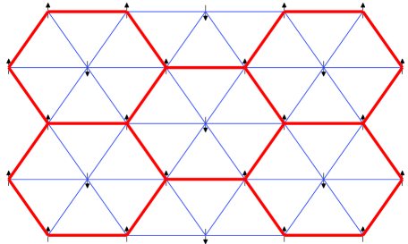
Figure 6: Maximally flippable configuration. Ising spins are shown on each site. Frustrated bonds are (bold) red, unfrustrated bonds (light) blue.

Now consider stacking this configuration antiferromagnetically. In a given plane, half of the sites are married to sites in the layer below, and the other half above. It follows then that we may flip half the sites on one sublattice along with their partners above and the other half with their partners below. This leads to a lower bound on the ground state entropy

$$S/N>(\log 2)/6$$ (19)

where $N$ is the total number of sites in the system. The scaling with $N$ establishes the macroscopic character of the ground state entropy. In contrast, for the STL there are only $N^{2/3}$ ground states. A simple upper bound

$$S_{u}/N<0.3383\ldots$$ (20)

is obtained by considering the entropy of decoupled triangular layers Wannier (1950).

We remark that a binary alloy that forms in the TS-FCC family of structures would thus be expected to exhibit a macroscopic zero temperature entropy, contributing to its stabilization.

III.3.2 Order by disorder

The next question to consider is whether the ground state manifold breaks any symmetries, i.e. whether the unweighted average over all the ground states yields long range order in the correlation functions.

What kind of order might one expect? As this order has to be selected entropically, i.e. by the preponderance of a family of configurations in the ground state average, we expect it to correspond to the configuration that has the greatest number of nearby configurations reached by local moves. The stacked maximally flippable (MF) configuration considered in our entropy lower bound meets this criterion—it is also the three dimensional configuration with maximal flippability. To see this, observe first that the constraint of inter-planar spin partnering is absolute in the ground state manifold: no spin may be flipped independently of its partner. Spin configurations which are stacked (the same in every layer) automatically partner flippable spins to flippable spins, and thus the stacking bonds impose no additional constraints on flippability. As the MF state maximizes the number of flippable spins in each plane, stacking this state gives the maximum possible number of flippable spins for the SSTL.

We should note however, that the spin distribution in the maximally flippable configuration is not directly observable; instead, it must be dressed by the fluctuations that select it. Two options emerge naturally. The first involves a three sublattice structure with magnetizations $(c,-c,0)$ wherein one of the two sublattices of flippable spins does all the flipping and thus exhibits a vanishing magnetization while the other two sublattices exhibit equal and opposite magnetizations. The other exhibits a three sublattice structure but now with two equivalent sublattices. The magnetizations $(d,-d^{\prime}/2-d^{\prime}/2)$ reflect more completely the symmetries of the maximally flippable configuration. The selection between these two is a matter of detail. The reader should note that both options give rise to six symmetry equivalent states.

Unfortunately, direct demonstration that one of these options is realized is not straightforward and we will not definitively answer this question in this paper although we believe that symmetry breaking in the $(c,-c,0)$ is realized at $T=0$. Instead we will, in the next section, approach the existence and structure of the ordered phase from the paramagnetic phase at high temperatures by constructing the appropriate LGW functional.

But before we do that let us briefly comment on the difference between what we have discussed here the corresponding analysis of the STL Ising antiferromagnet. On the STL, the ground state manifold exhibits long range order in the stacking direction but only algebraic order in the planes—in the latter directions it exhibits the known correlations of a single triangular layer Stephenson (1964). This algebraic order is again present at the wavevectors of the maximally flippable state (Fig 6). In the STL, switching on a small $T>0$ converts this to true long range order. The mechanism is “order by disorder” which can be visualized as the entropic dominance of three dimensional configurations in which flippable spins in the MF configurations in the planes stack with a set of mobile solitonic defects Coppersmith (1985); Moessner et al. (2000); Moessner and Sondhi (2001). In this setting it is by now clear that a single low temperature phase in the $(c,-c,0)$ pattern is separated from the paramagnet Kim et al. (1990); Moessner et al. (2001). The major qualitative difference between the STL and the SSTL is then that in the latter fluctuations in the stacking direction are present already at $T=0$ and so we expect that (eventually) the low temperature ordering can be understood by an analysis of the ground states alone.

III.3.3 LGW analysis

We now add another ingredient to our analysis of the Ising problem by applying the LGW and Renormalization group analysis to this case. This yields

$$\mathcal{H_{I}}= [ \!\!r+c_{\perp}(q_{x}^{2}+q_{y}^{2})+c_{z}q_{z}^{2}]\,\phi_{1}^{a}\overline{\phi}_{1}$$

$$+ u_{4}(\phi_{1}\overline{\phi}_{1})^{2}+u_{6}(\phi_{1}\overline{\phi}_{1})^{3}+v_{6}(\phi_{1}^{6}+\overline{\phi}_{1}^{6})$$

where we have now kept terms to sixth order in the fields. This is necessary for the second of these terms is the first one that breaks a $U(1)$/XY symmetry that is present up to fourth order down to a $Z_{6}$ (clock) symmetry. Consequently, there is a discrete set of six symmetry equivalent states at low temperatures and we reproduce a key feature of the Ising problem. The two possible signs of $v_{6}$ correspond to the two magnetization patterns discussed in above. This term is dangerously irrelevant: it is irrelevant at the critical fixed point that controls the transition into the broken symmetry phase, but to get the correct low-temperature physics it cannot be set to zero. Since it is irrelevant at the critical point, the transition is in the universality class of the three dimensional XY model. It is worth noting that a finite stack will exhibit a Kosterlitz-Thouless transition Isakov and Moessner (2003). All these results parallel those for the STL Blankschtein et al. (1984).

III.3.4 Monte Carlo results

The remaining challenge is to distinguish between the two ordering alternatives or equivalently, to fix the sign of $v_{6}$. As this is sensitive to microscopics, we have chosen to simulate the system to investigate this question.

In the simulations we used a simple spin-flip Monte Carlo algorithm. The algorithm allows 2 types of moves: a single spin flip, or a double spin flip which reverses a pair of partnered spins in adjacent layers. While this is sufficient for our purposes near the transition, at low temperatures it fails to be ergodic. The nature of the problem is clearest at zero temperature, where only the double spin flip is allowed. Hence a spin $s_{1}$ in a given triangular plane may be flipped only if its partner $s_{2}$ in the adjacent plane is also flippable. As only $2$ of the $6$ in-plane neighbours of $s_{1}$ are partnered with in-plane neighbours of $s_{2}$, at $T=0$ configurations exist in which this pair can be flipped only after flipping spins in all other layers of the system. Hence at low temperatures a more complicated, cluster-type method must be used. We expect to discuss such a method, and thus the ordering at low temperatures as well as a good estimate of the zero temperature entropy in a future publication Burnell and Sondhi .

We turn now to the data for systems of size $6\times 6\times 6$ and $12\times 12\times 12$ for the temperature ranges where our algorithm is ergodic as evidenced by the decay in single spin autocorrelations to zero. The system dimensions are chosen to be $N$ triangular planes of $N^{2}$ sites each with periodic boundary conditions in all directions.

For these systems we proceed as follows: In each configuration we compute and order the three sublattice magnetizations as $M_{1}>M_{2}>M_{3}$. We then compute the matrix of correlations $\langle M_{i}M_{j}\rangle$ averaged over the run. The results are shown in Fig 7. As the reader will note these correlators should, in the $(c,-c,0)$ state, exhibit the values $c^{2}$, $-c^{2}$ and $0$ in the infinite volume limit. Our computations are consistent with that and clearly inconsistent with the competing $(d,-d^{\prime}/2-d^{\prime}/2)$ state. This includes details such as the multiplicity of the values observed, and their evolution between the two system sizes.

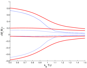
Figure 7: Correlations of sublattice magnetizations as functions of temperature, indicating the phase transition from 3 sublattice order to a paramagnetic state. Two lattice sizes are shown: a $6\times 6\times 6$ lattice in (light) blue, and a $12\times 12\times 12$ lattice in (bold) red.

IV Concluding Remarks

To summarize, we have studied nearest neighbor $O(N)$ antiferromagnets on an infinite subset of the new family of packings introduced by Torquato and Stillinger and established the nature of the ordering at low temperatures and the nature of the phase transitions.

We have done our analysis in the equivalent representation of the SSTL. This has the great advantage that we have dealt with the entire family of lattices at once—most of which have sizeable unit cells stemming from long periods in the stacking direction. However, for a specific realization, it will be necessary to translate the ordering back into the actual geometry of the lattice. For example, for the TS-FCC lattice the ordering wavevectors $\pm{4\pi\over 3}\hat{x}$ common to all $O(N)$ cases, translate into the vectors

$$\pm{2\pi\over a}\left(0,{\sqrt{3}\over 9},{\sqrt{6}\over 9}\right)$$

in the choices made in Equations (II) and (II).

One statistical mechanical remark may be interesting to readers. By this somewhat circular route we have discovered that the SSTL preserves the ordering of the STL for the Ising problem, while exhibiting a greatly increased ground state entropy. This analysis indicates that further dilution of the stacking bonds will further boost the zero temperature entropy while still preserving the nature of the ordered phase at asymptotically low temperatures.

Finally, we have taken a preliminary look at TS packings which are not in the TS-FCC class. The appear, generically, to be more frustrated than the ones studied in this paper and thus are an interesting topic for future work.

Acknowledgements: We are very grateful to Sal Torquato for introducing us to the Torquato-Stillinger packings. We would also like to thank Werner Krauth and Roderich Moessner for discussions on cluster and pocket algorithms. This work was supported in part by NSF Grant No. DMR 0213706 (SLS) and a NSERC fellowship (FJB).

References

- Ashcroft and Mermin (1976) N. Ashcroft and N. Mermin, Solid State Physics (Brooks/Cole, 1976), chapter 4.
- Anderson (1950) P. W. Anderson, Phys. Rev. 79, 705 (1950).
- Luttinger (1951) J. M. Luttinger, Phys. Rev. 81, 1015 (1951).