Phase diagram of a 2D Ising model within a nonextensive approach

Abstract

In this work we report Monte Carlo simulations of a 2D Ising model, in which the statistics of the Metropolis algorithm is replaced by the nonextensive one. We compute the magnetization and show that phase transitions are present for $q\neq 1$. A $q\,-$ phase diagram (critical temperature vs. the entropic parameter $q$) is built and exhibits some interesting features, such as phases which are governed by the value of the entropic index $q$. It is shown that such phases favors some energy levels of magnetization states. It is also showed that the contribution of the Tsallis cutoff is essential to the existence of phase transitions.

¹ Centro Brasileiro de Pesquisas Físicas, Rua Dr. Xavier Sigaud 150, 22290-180, Rio de Janeiro, Brazil
² CICECO, Universidade de Aveiro, 3810-193, Aveiro, Portugal

1 Introduction

The nonextensive statistics is a generalization of the Boltzmann – Gibbs one and it is based on the nonadditive entropy [1]

$$S_{q}=k\frac{1-\sum_{i}p_{i}^{q}}{q-1}\qquad(q\,\in\,\Re)$$ (1)

where $q$ is the entropic index for a specific system, connected to its dynamics, as recently proposed [2, 3]; $p_{i}$ are probabilities satisfying $\sum_{i}p_{i}=1$, $k$ is a constant, and $\lim_{q\rightarrow 1}S_{q}=S_{BG}$, where $S_{BG}$ is the Boltzmann – Gibbs entropy. In this statistics, a system composed of two independent parts $A$ and $B$, in the sense that the probabilities of the systems factorize, has the following pseudo-additivity (nonextensivity) property of the entropy [4, 5]

$$S_{q}(A+B)=S_{q}(A)+S_{q}(B)+(1-q)\,S_{q}(A)\,S_{q}(B)/k.$$ (2)

This pseudo-additivity is related to the composability property of $S_{q}$ [6]. Since for any system $S_{q}\geq 0$, then $q<1$ correspond to superadditivity (superextensivity), $q=1$ to additivity (extensivity), and $q>1$ to subadditivity (subextensivity). Besides representing a generalization, $S_{q}$, as much as $S_{BG}$, is positive, concave and Lesche-stable ($\forall\,q>0$). Recently, it has been shown that it is also extensive for some kinds of correlated systems in which scale invariance prevails [7, 8].

In this paper we report some results of a Monte Carlo simulation of a 2D Ising model upon replacing the statistics of the Metropolis algorithm by the nonextensive statistics. From numerical calculations we compute the magnetization of the system, and built a $q\,-$ phase diagram showing that, even for $q\neq 1$, exist phase transitions, in contrast to a previous work [9]. The text is organized as follows: In Section 2, we describe the equilibrium distribution of nonextensive statistics and the importance of the internal energy constrains. In Section 3, we describe the introduction of the nonextensive formalism into the Monte Carlo method. In Sections 4 and 5, we discuss the main results and describe the behavior of the critical temperature with the entropic index in a phase diagram ($T_{c}$ vs. $q$).

2 Nonextensive statistics

To calculate the equilibrium distribution, the above entropy, Eq.(1), must be maximized [1]. If the system is isolated, i.e., in a microcanonical ensemble,

$$\sum_{i=1}^{\Omega}p_{i}=1$$ (3)

the maximization yields equiprobability of states occupation. On the other hand, if the system is in contact with a thermal reservoir (canonical ensemble), it is necessary to add the internal energy constraints, which can be done according to three possible choices. The first one is [1]

$$\sum_{i=1}^{\Omega}p_{i}\,\varepsilon_{i}=U$$ (4)

the standard definition of internal energy in which $\{\varepsilon_{i}\}$ are the eigenvalues of the Hamiltonian of the system. The second, as postulated in [10], is:

$$\sum_{i=1}^{\Omega}p_{i}^{q}\varepsilon_{i}=U_{q}.$$ (5)

Both definitions presents some difficulties with the interpretation of some results [11]. Thus, a third choice for the internal energy constraint was introduced as [11]:

$$\frac{\sum_{i=1}^{\Omega}p_{i}^{q}\varepsilon_{i}}{\sum_{i=1}^{\Omega}p_{i}^{q}}=U_{q}$$ (6)

which defined the escort probability (first introduced in Ref. [12]):

$$P_{i}^{(q)}\equiv\frac{p_{i}^{q}}{\sum_{j=1}^{\Omega}p_{j}^{q}}.$$ (7)

The maximization of $S_{q}$ in that case yields for the probability distribution

$$p_{i}=\frac{1}{Z_{q}}\,\left[1-\frac{(1-q)\,\beta\,(\varepsilon_{i}-U_{q})}{\sum_{j=1}^{\Omega}p_{j}^{q}}\right]^{1/(1-q)}$$ (8)

where

$$Z_{q}=\sum_{i=1}^{\Omega}\left[1-\frac{(1-q)\,\beta\,(\varepsilon_{i}-U_{q})}{\sum_{j=1}^{\Omega}p_{j}^{q}}\right]^{1/(1-q)}$$ (9)

is the nonextensive partition function and $\beta$ a Lagrange multiplier. After some algebraic manipulations [11] it becomes:

$$p_{i}=\frac{1}{Z_{q}^{\prime}}\,\left[1-(1-q)\,\beta^{\prime}\,\varepsilon_{i}\right]^{1/(1-q)}=\frac{1}{Z_{q}^{\prime}}\,e_{q}^{-\beta^{\prime}\varepsilon_{i}}$$ (10)

and

$$Z_{q}^{\prime}=\sum_{j=1}^{\Omega}\left[1-(1-q)\,\beta^{\prime}\,\varepsilon_{j}\right]^{1/(1-q)}=\sum_{j=1}^{\Omega}e_{q}^{-\beta^{\prime}\varepsilon_{i}}$$ (11)

where

$$\beta^{\prime}=\frac{\beta}{\sum_{j=1}^{\Omega}p_{j}^{q}+(1-q)\,\beta\,U_{q}}.$$ (12)

and $e_{q}^{x}$ is the generalized exponential, which has the following the property:

$$[1-(1-q)\,\beta^{\prime}\varepsilon_{i}]^{1/(1-q)}=\left\{\begin{array}[]{ll}e_{q}^{-\,x},&\mbox{if $1-(1-q)\,x\geq 0$};\\ 0,&\mbox{if $1-(1-q)\,x<0$}.\end{array}\right.$$ (13)

known as the Tsallis cutoff procedure. A detailed discussion about the role of constraints within the nonextensive statistics was done by Tsallis et al [11], but recently it has been showed by Ferri et al [13] the equivalence of all these formulations of internal energy constraints. In spite of that, in this work, to avoid misunderstanding, we choose the normalized internal energy form.

The thermal equilibrium in the nonextensive statistics is still an open issue due to the definition of the physical temperature [14, 15, 16, 17, 18, 19, 20]. Thus, differently from some authors [9], in our approach the parameter $\beta^{\prime}$ is assumed to be the physical temperature, i.e., $\beta^{\prime}=(k\,T)^{-1}$. The validity of this choice was first shown experimentally [21], and latter theoretically [2, 3, 22, 23] for manganites.

3 Monte Carlo simulations of a 2D Ising model using nonextensive statistics

In this section we are going to discuss the modification of the Metropolis method for the nonextensive statistics, considering a ferromagnetic 2D Ising with first-neighbors interaction. The Hamiltonian is given by

$$\mathcal{H}=-J\sum_{\langle ij\rangle}s_{i}s_{j}$$ (14)

where $\langle ij\rangle$ denotes the sum over first neighbors on a square lattice of size $N=L\times L$, $s_{i}=\pm 1$ and $J>0$ (ferromagnetic interaction). We proceed the single flip Monte Carlo calculations [24] to obtain the magnetization of the system, however we have changed the usual statistical weight to:

$$w=\frac{P_{i,after}^{(q)}}{P_{i,before}^{(q)}}=\left[\frac{e_{q}^{-\varepsilon_{i}^{after}/k\,T}}{e_{q}^{-\varepsilon_{i}^{before}/k\,T}}\right]^{q}$$ (15)

or, in other words, the ratio between the escort probabilities before and after the spin flip. Since this quantity is a ratio, the normalization factor of the escort probabilities, i.e., the generalized partition function, Eq.(11), cancels and the weight calculated can be written as the ratio between the generalized exponentials raised to the entropic parameter $q$. It is important to emphasize that $w$ is the quantity that will be compared to a random number in the Metropolis algorithm (see appendix for details on the MC procedure used). It is also important to note that the Tsallis cutoff procedure, Eq.(13), must be taken into account, i.e., it must be included into $w$ to avoid complex probabilities. The simulations were done with the entropic parameter $q\in[0,1]$. Lattice size were $L=8,16,24,32$, with periodical boundary condition imposing that $s_{L+1}\equiv s_{1}$.

4 Results and Discussion

The most probable normalized magnetization, $m=M/L^{2}$, was obtained after $5\times 10^{5}$ Monte Carlo steps and are shown on Fig.(1) for $q=0.4$, $q=0.7$ (which are representative results for $q<0.5$ and $q>0.5$, respectively), and for $q=1$. One can observe that for $q>0.5$ there are strong influences of the lattice size on the shape of the magnetization curve and on the critical temperature, $T_{c}$. In addition, the magnetization drops smoothly to zero close to $T_{c}$ due to the thermal fluctuations. On the contrary, for $q<0.5$, there are no dependence of those quantities on the lattice size, and the magnetization changes suddenly at $T_{c}$, from $m=1$ to $m=0$. In other words, there are no thermal fluctuations in this case and the magnetization works like a microcanonic two-level system.

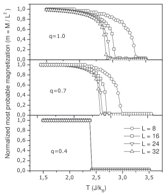
Figure 1: Normalized most probable magnetization vs. temperature. For $q=0.4$ it can be seen that the magnetization has no dependence on the lattice size, dropping form $m=1$ to $m=0$ suddenly at $T_{c}$. It happens due to the contribution of the Tsallis cutoff. However, for $q=0.7$ the magnetization depends on the lattice size and smoothly goes to zero close to $T_{c}$ as a second order phase transition. For $q=1$ it recovers the well known result.

This behavior, for $q<0.5$, is simple to be understood. At low temperatures (for instance $T=1.5$ and $q=0.4$), the first Monte Carlo steps lead the magnetization to $m=1$, i.e., to the ground state, as expected (due to the low temperatures). Then the subsequent Monte Carlo steps attempt to invert the spin, but it fails because is energetically unfavorable. Then the Metropolis algorithm takes place; as $\varepsilon_{i}^{after}=4\,J$ and $\varepsilon_{i}^{before}=-4\,J$, therefore $1-(1-q)\,\beta^{\prime}\,\varepsilon_{i}^{after}<0$ for all $T<4\,J\,(1-q)$. So, considering the cutoff, Eq.(13), $p_{i}^{after}=0$ and then $w=0$. Since the Metropolis algorithm flips energetically unfavorable spins if the random number is smaller then $w$, for $T<4\,J\,(1-q)$ those spins never flips ($w=0$), keeping the magnetization at $m=1$; in other words, in the ground state. This situation persists up to $T_{c}=4\,J\,(1-q)$, where the cutoff for $p_{i}^{after}$ is no longer satisfied and the thermal fluctuation can therefore acts. However, the spins are already quite warm and the magnetization drops suddenly to zero, i.e., to a equiprobable state. A similar behavior was already found describing the generalized Brillouin function [22].

To determine the critical temperature we must take the thermodynamic limit ($L\rightarrow\infty$). In Fig.(2) we plot the critical temperature as a function of the inverse lattice size for different values of the entropic parameter, taking the limit ($L^{-1}\rightarrow 0$). Notice that the critical temperature for $q=1$ tends to Onsager result and, as explained above, it does not depend on the lattice size for $q<0.5$. Similar independency were found in different systems [25]. Also, the slope of the curves changes with the entropic parameter $q$, suggesting a dependence of the critical exponents on the entropic parameter (for studies about this connection see for example [26, 27, 28]).

With those critical temperature values we build a phase diagram shown in Fig.(3), i.e., $T_{c}$ as a function of $q$. It is quite interesting because, in contrast to previous works [9], we found that for the Monte Carlo simulations of a 2D Ising model in nonextensive statistics has phase transitions for $q\neq 1$. It is clear that below the $4\,J\,(1-q)$ line the system is in the ground state and then $m=1$. Above this line there are two regions where the thermal fluctuation act: one above $T_{c}$, i.e., in the paramagnetic regime and, consequently, in the equiprobable state; and the other regime lies between $4\,J\,(1-q)$ line and $T_{c}$ when the magnetization assume values between 0 and 1. It is interesting that the slope of the critical temperature, $T_{c}(q)$, does not changes abruptly with the increase of the entropic parameter. For $q\sim 0.5$ the slope changes smoothly indicating that the spin is not warm enough and pass to a thermal distribution region before the equiprobable state.

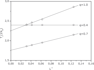
Figure 2: Taking the thermodynamical limit of the system, one can notice that the behavior is quite different for $q<0.5$ and for $q>0.5$. As can be seen, for $q=0.4$ the critical temperature has no dependence on the lattice size. It happens due to the contribution of the Tsallis cutoff. However, for $q=0.7$ the lattice size dependence appears. For $q=1$ the thermodynamical limit recovers the critical temperature of Onsager result ($T_{c}=2\,[\arctan(1/\sqrt{2})]^{-1}$).

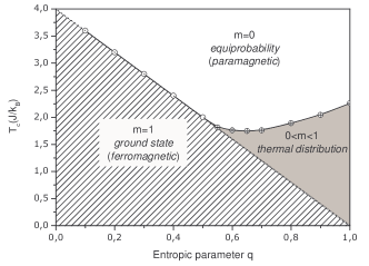
Figure 3: Three different regions can be seen in this $q\,-$ phase diagram. The first one is the ferromagnetic ground state ($m=1$) which is kept from zero Kelvin until $T_{c}=4\,J\,(1-q)$, due to the contribution of the Tsallis cutoff. The second region has influence at the thermal distribution ($0<m<1$). The third is the equiprobable paramagnetic state ($m=0$). The error is smaller then the the size of those dots.

5 Conclusions

In this work, we studied a ferromagnetic 2D Ising model with first-neighbor interactions through a Monte Carlo simulation in which the Metropolis algorithm was changed to the nonextensive statistics. Magnetization as a function of the temperature for different values of $q$ were evaluated and we found phase transition for $q\neq 1$, in contrast to a previous work [9]. This results arises due to the definition of the physical temperature. In addition, we also have showed the contribution of the Tsallis cutoff is of great importance and rules the phase transition for $q<0.5$.

The authors acknowledge S.M.D. Queirós, C. Tsallis and R. Toral for their comments. We would like to thanks the Brazilian funding agencies CNPq and CAPES. DOSP would like to thanks the Brazilian funding agency CAPES for the financial support at Universidade de Aveiro at Portugal.

Appendix

Each Monte Carlo step can be resumed as the following

1. Compute the interaction energy of a given spin $i-$th of the lattice with its neighbors $\varepsilon_{i}^{before}=\sum_{j=1}^{4}\varepsilon_{ij}$. After that, change the state of this spin and compute again its interaction energy, $\varepsilon_{i}^{after}$. If $\varepsilon_{i}^{after}<\varepsilon_{i}^{before}$, accept the change of state;

2. If the energy is not lower, using Eq.(13), compute $w$. Compare this quantity to a number that belongs to the interval $[0,1]$ generated randomly. Being this random number smaller then $w$ then accept the change of state, otherwise not.

As can be seen, this is the ordinary Metropolis algorithm in which the probability of state was changed from the Boltzmann weight to the Tsallis factor, Eq.(7).

References

- [1] C. Tsallis. Possible generalization of Boltzman-Gibbs statistics. Journal of Statistical Physics, 52:479, 1988.
- [2] M. S. Reis, V. S. Amaral, R. S. Sarthour, and I. S. Oliveira. Experimental determination of the nonextensive entropic parameter q. Physical Review B, 73:092401, 2006.
- [3] M. S. Reis, V. S. Amaral, R. S. Sarthour, and I. S. Oliveira. Physical meaning and measurement of the entropic parameter q in an inhomogeneous magnetic systems. European Physical Journal B, 50:99, 2006.
- [4] C. Tsallis. Nonextensive Statistics: Theoretical, Experimental and Computational Evidences and Connections. Brazilian Journal of Physics, 29:1, 1999.
- [5] C. Tsallis and E. Brigatti. Nonextensive statistical mechanics: A brief introduction. Continuum Mechanics and Thermodynamics, 16:223, 2004.
- [6] C. Tsallis. Nonextensive Entropy - Interdisciplinary Applications, chapter Nonextensive statistical mechanics: Construction and physical interpretation. eds. M. Gell-Mann and C. Tsallis. Oxford University Press, New York, 2004.
- [7] C. Tsallis, M. Gell-Mann, and Y. Sato. Asymptotically scale-invariant occupancy of phase space makes the entropy Sq extensive. Proceedings of the National Academy of Science, 102:15377, 2005.
- [8] For a complete and updated list of references, see the web site: tsallis.cat.cbpf.br/biblio.htm.
- [9] A. R. Lima, J. S. S. Martins, and T. J. P. Penna. Monte Carlo Simulation of Magnetic System in the Tsallis Statistics. Physica A, 268:553, 1999.
- [10] E. M. F. Curado and C. Tsallis. Generalized statistical mechanics: connection with thermodynamics. Journal of Physics A, 24:L69, 1991. Corrigenda: 24 (1991) 3187 and 25 (1992) 1019.
- [11] C. Tsallis, R. S. Mendes, and A. R. Plastino. The role of constraints within generalized nonextensive statistics. Physica A, 261:534, 1998.
- [12] C. Beck and F. Schlogl. Thermodynamics of Chaotic Systems: An Introduction. Cambridge University Press, Cambridge, 1993.
- [13] G. L. Ferri, S. Martínez, and A. Plastino. Equivalence of the four versions of Tsallis’s statistics. Journal of Statistical Mechanics: Theory and Experiment, 4:P04009, 2005.
- [14] R. Salazar and R. Toral. A Monte Carlo Method for the Numerical Simulation of Tsallis Statistics. Physica A, 283:59, 2000.
- [15] S. Martínez, F. Pennini, and A. Plastino. The concept of temperature in a nonextensive scenario. Physica A, 295:246, 2001.
- [16] S. Martínez, F. Pennini, and A. Plastino. Thermodynamics’ zeroth law in a nonextensive scenario. Physica A, 295:416, 2001.
- [17] R. Toral and R. Salazar. Ensemble equivalence for non-extensive thermostatistics. Physica A, 305:52, 2002.
- [18] R. Toral. On the definition of physical temperature and pressure for nonextensive thermostatistics. Physica A, 317:209, 2003.
- [19] Q. A. Wang, L. Nivanen, A. LeMéhauté, and M. Pezeril. Temperature and pressure in nonextensive thermostatistics. Europhysics Letters, 65:606, 2004.
- [20] S. Abe. Temperature of nonextensive systems: Tsallis entropy as Clausius entropy. Physica A, 368:430, 2006.
- [21] M. S. Reis, J. C. C. Freitas, M. T. D. Orlando, E. K. Lenzi, and I. S. Oliveira. Evidences for Tsallis non-extensivity on CMR manganites. Europhysics Letters, 58:42, 2002.
- [22] M. S. Reis, J. P. Araújo, V. S. Amaral, E. K. Lenzi, and I. S. Oliveira. Magnetic behavior of a nonextensive S-spin system: Possible connections to manganites. Physical Review B, 66:134417, 2002.
- [23] M. S. Reis, V. S. Amaral, J. P. Araújo, and I. S. Oliveira. Magnetic phase diagram for a nonextensive system: Experimental connection with manganites. Physical Review B, 68:014404, 2003.
- [24] R. H. Landau and M. J. Paez. Computational Physics: Problem solving with computers. Wiley-VHC, Weinheim, 2004.
- [25] I. Bediaga, E. M. F. Curado, and J. M. de Miranda. A nonextensive thermodynamical equilibrium approach in hadrons. Physica A, 286:156, 2000.
- [26] R. Salazar and R. Toral. Scaling Laws for a System with Long-Range Interactions within Tsallis Statistics. Physical Review Letters, 83:4233, 1999.
- [27] R. Salazar, A. R. Plastino, and R. Toral. Weakly nonextensive thermostatistics and the Ising model with long-range interactions. European Physical Journal B, 17:679, 2000.
- [28] R. Salazar and R. Toral. Thermostatistics of extensive and non-extensive systems using generalized entropies. Physica A, 290:159, 2001.