RADIATION PRESSURE SUPPORTED AGN TORI WITH HARD X-RAY AND STELLAR HEATING

Abstract

The dynamics and structure of toroidal obscuration around AGN remain uncertain and controversial. In this paper we extend earlier work on the dynamical role of infrared radiation pressure by adding the effects of two kinds of distributed heating: Compton-heating due to hard X-rays from the nucleus and local starlight heating. We find numerical solutions to the axisymmetric hydrostatic equilibrium, energy balance, and photon diffusion equations including these effects. Within the regime of typical parameters, the two different sources of additional heating have very similar effects: the density profile within the torus becomes shallower both radially and vertically, but for plausible heating rates, there is only minor change (relative to the source-free case) in the distribution of column density with solid angle. The most interesting consequence of distributed heating is that it selects out a relatively narrow range of parameters permitting an equilibrium, particularly $(L/L_{E})/\tau_{T}$. We discuss the implications of both the narrowness of the permitted range and its approximate coincidence with the range inferred from observations.

1 INTRODUCTION

The obscuring torus is one of the key components to the anisotropic appearance of AGN. Although much observational evidence exists to directly (e.g. Jaffe et al., 2004) or indirectly (e.g. Barthel, 1989; di Serego Alighieri et.al., 1994; Zakamska et al., 2005) confirm the existence of this structure, there is little understanding of its dynamics. The central question is the nature of the mechanism that supports the torus’s large geometrical thickness against gravity.

Numerous ideas have been proposed to answer this question. The first suggestion was the clumpy torus model (Krolik & Begelman, 1988). In that model, the torus consists of highly clumped gas and dust, and the clumps undergo highly supersonic motions. To avoid rapid collisional loss of kinetic energy, a large magnetic field is needed to ensure that each collision is sufficiently elastic. Königl & Kartje (1994) presented another possible approach. In their model, they argued that a magneto-centrifugal wind could replace the torus. However, this model faces difficulties to explain the origin of the large-scale magnetic field and the source of the large energy needed to drive the wind. Another possibility is that the support is from radiation pressure (Pier & Krolik, 1992a). The optical through soft X-ray continuum of the nucleus is absorbed and re-emitted in infrared light by dust at the inner edge of the torus; then the large opacity in that band couples the radiation flux to the gas and provides a strong radiation force to balance the gravity. Following this basic idea, Krolik (2007, hereafter K07) constructed an idealized model, and via this model found self-consistent hydrostatic equilibrium solutions analytically. These solutions demonstrate that infrared radiation pressure is able to support the geometrically thick structures around AGN. For simplicity, that work did not consider any internal sources of heating, such as the Compton heating due to hard X-rays penetrating the torus interior, or the heating from local starlight irradiating the dust. Both of them contribute a positive divergence of flux to the energy equation, which can strongly affect the configuration of the torus and even the existence of equilibrium solutions.

It is the object of this paper to construct a generalized radiation support model by including these local heating mechanisms. We first construct the physical model in section 2, introducing the basic equations and assumptions adopted in this work. Section 3 shows how we solve these equations. After defining dimensionless parameters and identifying appropriate boundary conditions, we describe in detail the numerical method implemented in this work. The results and discussion are presented in section 4, and the conclusions follow in section 5.

2 THE PHYSICAL MODEL

We choose 2-d axisymmetric geometry to explore this picture. All physical quantities are written in cylindrical coordinates on the $r-z$ plane. To be appropriate to flattened geometries, three simplifying assumptions are adopted. First, we take $\Omega$ as the local orbital frequency, which at all heights z equals the rotation rate of a circular orbit in the torus midplane at radius $r$. Second, we follow only the component of angular momentum parallel to the torus axis, and we assume that the gas’s specific angular momentum has magnitude $jr^{2}\Omega$ with $j=j(r,z)\leq 1$. Third, the radial and vertical components of gravity are approximated by $r\Omega^{2}$ and $z\Omega^{2}$. In fact, $\Omega(r,|z|>0)<\Omega(r,z=0)$, so this approximation slightly overestimates the strength of gravity. For example, in a point mass potential, $\Omega^{2}(r,z)=GM_{\scriptscriptstyle{BH}}/(r^{2}+z^{2})^{3/2}\leq\Omega^{2}(r,z=0)$, where $M_{\scriptscriptstyle{BH}}$ denotes the mass of the central black hole. We also assume the interior of the torus is in hydrostatic equilibrium, so that:

$$\kappa\mathbf{F}/c=-\mathbf{g}_{eff}=r\Omega^{2}(1-j^{2})\textbf{e}_{r}+z\Omega^{2}\textbf{e}_{z},$$ (1)

where the infrared radiation flux is $\mathbf{F}$, $\kappa$ is the opacity per unit mass, and $\mathbf{g}_{eff}$ is the net gravity.

Instead of solving a complete transfer problem at all relevant frequencies for all photon directions, we approximate the radiation flux by solving the diffusion equation with a thermally-averaged opacity. In this approximation, the flux is obtained from the gradient of the radiation energy density:

$$\mathbf{F}=-\frac{c}{3\kappa\rho}\nabla E,$$ (2)

where $\rho$ is the gas mass density and $E$ is the radiation energy density.

If the only source of infrared radiation is the conversion via dust reradiation of optical and UV photons at the inner edge of the torus, then in the body of the torus

$$\nabla\cdot\mathbf{F}=0.$$ (3)

However, the existence of distributed sources in the torus is also possible. For instance, when hard X-rays penetrate deeply into the torus material, local heating due to Compton recoil (e.g., Chang et al., 2007) can be considerable. It is also possible that local star formation is sufficiently strong that stellar luminosity may supplement the AGN’s radiation force (see Thompson et al., 2005).

In this paper, we explore both of these. In the former case, if the torus is optically thin to hard X-rays, a more general formula to describe the energy conservation reads

$$\nabla\cdot\mathbf{F}=\frac{L_{X}}{4\pi(r^{2}+z^{2})}n_{e}\sigma_{T}f_{c},$$ (4)

where $L_{X}$ is the luminosity in hard X-rays, $n_{e}$ is the electron number density, and $f_{c}$ is the ratio of the energy gained by electrons during each collision to the photon energy. Even bound electrons behave as if they are free when scattering X-rays with energy greater than roughly 3-4 keV (Krolik, 1999), and Klein-Nishina effects are negligibly small for hard X-ray photons $<100$keV, thus $\sigma_{T}$, the Thomson cross section, is the appropriate cross section.

We have much more freedom to choose the distribution of internal starlight. A reasonable assumption is to adopt the Schmidt Law that the star formation rate is proportional to the $3/2$-power of the gas density (Kennicutt, 1998), and assume that the local stellar luminosity is proportional to the star formation rate. Due to the large optical depth to the UV and optical, the stellar radiation is assumed to be absorbed in situ and reproduced in the infrared. As in equation 4, we can write the equation of energy conservation including local stellar heating as

$$\nabla\cdot\mathbf{F}=S\left(\frac{\rho}{\rho_{in}}\right)^{3/2},$$ (5)

where $S$ is a coefficient with units of erg cm^-3 s^-1 which describes the strength of the sources, and $\rho_{in}=\rho(r_{in},0)$ is the gas density along the inner edge of the torus ($r=r_{in}$) measured on the midplane.

With equations 1,2 and either 4 or 5, it is possible to solve for all three unknowns, $\mathbf{F}$, $E$ and $\rho$.

3 THE GENERALIZED SOLUTIONS

3.1 Preparatory Work

To find the energy density and matter density from the three equations introduced in the last section, we need to combine them and simplify them.

Putting the flux equation 2 together with the hydrostatic equilibrium equation 1, we have

$$-\frac{1}{3\rho}\nabla E=r\Omega^{2}(1-j^{2})\textbf{e}_{r}+z\Omega^{2}\textbf{e}_{z}$$ (6)

which relates the energy density to the dynamics.

Combining equation 1 and either 4 or 5, one gets the relation between the dynamics and the local sources of heat:

$$\nabla\cdot\left\{\frac{c}{\kappa}[r\Omega^{2}(1-j^{2})\textbf{e}_{r}+z\Omega^{2}\textbf{e}_{z}]\right\}=\mathit{R},$$ (7)

where $\mathit{R}=n_{e}\sigma_{T}f_{c}L_{X}/{4\pi(r^{2}+z^{2})}$ in the case of hard X-ray heating and $\mathit{R}=S\left({\rho}/{\rho_{in}}\right)^{3/2}$ in the stellar heating case. According to the most recent dust opacity models (e.g., Semenov et al., 2003), the Rosseland mean opacity is a mildly changing function of the temperature in the range $100-1000$ K, which is also the interior temperature of the obscuring tori as found by detailed radiation transfer studies (Pier & Krolik, 1992b; Efstathiou & Rowan-Robinson, 1995; Granato et al., 1997; Nenkova et al., 2002). On this ground, we approximate $\kappa$ as constant. Equation 7 then reduces to

$$r\frac{\partial j^{2}}{\partial r}+2(1-\alpha)j^{2}+(2\alpha-3)=-\frac{\kappa}{c\Omega^{2}}\mathit{R},$$ (8)

where $\alpha$ is defined by $\Omega(r)=\Omega_{in}(r/r_{in})^{-\alpha}$ in order to allow for more general potentials than that of a simple point-mass. $\Omega_{in}=\Omega(r_{in})$ in that definition represents the orbital frequency measured on the inner edge of the torus. Without terms on the right hand side, we can solve equation 8 easily because there is no longer any dependence on $z$. When $\mathit{R}\neq 0$, we can treat the right hand side as a perturbation and solve the exact equation iteratively. Detailed description of this method will be given in subsection 3.4.

Once $j^{2}(r,z)$ is found, we can turn back to equation 6 and separate it into two equations:

$$\rho=-\frac{1}{3z\Omega^{2}}\frac{\partial E}{\partial z}=-\frac{1}{3r\Omega^{2}(1-j^{2})}\frac{\partial E}{\partial r}.$$ (9)

The second equality in the above equation allows us to rewrite the partial differential equation in characteristic form

$$\frac{dE}{ds}=\frac{\partial E}{\partial z}\frac{dz}{ds}+\frac{\partial E}{\partial r}\frac{dr}{ds}=0,$$ (10)

with

$$\frac{dz}{ds}=\frac{1}{z}~{},~{}~{}~{}~{}\frac{dr}{ds}=-\frac{1}{r(1-j^{2})}.$$ (11)

¿From the characteristic form, we find E is constant along contours parameterized by $\lambda$:

$$\frac{1}{2}z^{2}+\int_{r_{*}}^{r}dr^{\prime}r^{\prime}[1-j^{2}(r^{\prime},z)]=\lambda,$$ (12)

where $r_{*}$ is arbitrary.

However, to find the exact values of $E=E(r,z)$ at distinct locations, we need to know the energy density $E(\lambda)$ along any path on which $\lambda$ varies monotonically. For convenience, we can pick the path to run outward along the $r$ axis starting from the radius of the inner edge $r_{in}$. We then have

$$\frac{dE}{d\lambda}=\frac{\partial E}{\partial r}\frac{dr}{d\lambda}=-3\rho\Omega^{2}.$$ (13)

In order to achieve a solution, this equation requires advance knowledge of $\rho(\lambda)$ on its path. It is convenient in this context (in which we have already written $\Omega\propto r^{-\alpha}$) to consider density boundary conditions that also have power-law dependence on radius, i.e. $\rho(r,0)=\rho_{in}(r/r_{in})^{-\gamma}$. With this choice of gas density, the energy density can be easily found by integrating

$$\frac{dE(r,0)}{dr}=-3\rho(r,0)r\Omega^{2}[1-j^{2}(r,z)],$$ (14)

that is

$$E(r,0)=E_{in}-\int^{r}_{r_{in}}3\rho(r^{\prime},0)r^{\prime}\Omega^{2}[1-j^{2}(r^{\prime},0)]dr^{\prime},$$ (15)

where $E_{in}$ is the energy density measured at point $(r_{in},0)$. Thus, given $j^{2}$, which is the solution of equation 8, the density along the equatorial plane, and the energy density on the equatorial plane, the complete solution for $E$ can be achieved with equations 12 and 15. The matter density $\rho=\rho(r,z)$ can then be computed from either equality of equation 9.

3.2 Governing Parameters

We have mentioned two important dimensionless parameters in the previous subsection: $\alpha$ and $\gamma$. They determine the shape of the gravitational potential and the density profile on the equatorial plane. Besides those two, we still need several others to parameterize our problem. One of these is $j_{in}$, defined as $j_{in}=j(r_{in},0)$, which indicates the rotational support at the inner edge. Greater $j_{in}$ means that the torus requires a smaller radial thickness to reach the full Keplerian angular momentum. Another parameter is $\tau_{*}\equiv\kappa\rho_{in}r_{in}$, which sets the optical depth scale. If the density declines outward, $\tau_{*}$ must be at least several to satisfy the diffusion approximation. Because the Rosseland mean opacity of dust per unit mass of gas is $\sim 10$ – 30 times as great as the Thomson opacity per unit mass for temperature in the range 100-1000 K (Semenov et al., 2003), $\tau_{T}\equiv\kappa_{T}\rho_{in}r_{in}\sim(0.03-0.1)\tau_{*}$. For simplicity, $\tau_{T}=0.05\tau_{*}$ and $\tau_{*}=10$ (so that $\tau_{T}=0.5$) are adopted in this paper if we do not say otherwise.

We also need a parameter $Q\equiv 3\rho_{in}r^{2}_{in}\Omega^{2}_{in}/E_{in}$ to relate the orbital energy to the radiation energy. If no local heating exists in the torus, or the extra sources are negligibly weak, then the only contribution to $E_{in}$ is the absorbed radiation of the nucleus, which is mainly in the UV band. Thus we can write $E_{in}\sim L_{\scriptscriptstyle{UV}}h/(4\pi r_{in}^{2}c)$, where $L_{\scriptscriptstyle{UV}}$ denotes the luminosity of the nucleus in the UV, and $h$ is a blanketing factor, telling us by what factor the inner edge energy density is enhanced compared to what it would be in vacuum. However, the local heating also contributes to the energy density, and therefore we have

$$E_{in}=\frac{L_{\scriptscriptstyle{UV}}h}{4\pi r_{in}^{2}c}+\int\!\!\!\int drdz\frac{r\mathit{R}\,e^{-\tau(r,z)}}{[(r-r_{in})^{2}+z^{2}]c}=\frac{L_{\scriptscriptstyle{UV}}h}{4\pi r_{in}^{2}c}f_{*}.$$ (16)

The integral over the torus gives the contribution to the energy density due to the local sources. Here we assume the gas is axisymmetrically distributed and $\tau(r,z)$ is the infrared optical depth from the location of the source to the position $(r_{in},0)$. $f_{*}$ is a correction factor $\gtrsim 1$. With $E_{in}$ defined this way, the parameter $Q$ can be easily rewritten in terms of more familiar quantities:

$$Q=3\frac{\tau_{*}}{f_{*}h}\frac{M(<r_{in})}{M_{\scriptscriptstyle{BH}}}\frac{\kappa_{T}}{\kappa}\frac{L_{E}}{L_{\scriptscriptstyle{UV}}},$$ (17)

where $M(<r_{in})$ is the total mass interior to $r_{in}$, and $L_{E}$ is the Eddington luminosity. As discussed in K07, if $\tau_{*}\sim 10$–30, and the blanketing factor $h\gtrsim 2$, then reasonable values of $Q$ would be $\sim 0.1-10$.

The last two parameters characterize the internal sources. Firstly, the X-ray heating requires a parameter $X\equiv L_{X}f_{c}/(L_{\scriptscriptstyle{UV}}f_{*})$. Combining this definition with equation 16, we find that the correction factor $f_{*}$ is

$$f_{*}=\left[1-\frac{\tau_{T}X}{h}\,\mathit{I_{1}}\right]^{-1},$$ (18)

where $\mathit{I_{1}}=\int\!\!\int drdz\,(\rho/\rho_{in})(r/r_{in})e^{-\tau(r,z)}/\{[(r-r_{in})^{2}+z^{2}][(r/r_{in})^{2}+(z/r_{in})^{2}]\}$. Consequently, in terms of $X$, the ratio of the hard X-ray luminosity to the total luminosity from the nucleus is:

$$\frac{L_{X}}{L}\simeq\frac{L_{X}}{L_{X}+L_{\scriptscriptstyle{UV}}}=\frac{1}{1+f_{c}/(f_{*}X)}.$$ (19)

In AGN hard X-ray spectra, the photon spectral index ranges from $\sim 1$–3 (Beckmann et al., 2006; Tozzi et al., 2006); the averaged fractional energy lost $f_{c}=<\!\!h\nu/m_{e}c^{2}\!\!>$ is then $\sim 0.1$. Using the fact that bolometric corrections for $2-10$ keV X-rays are $\sim 8$–60 (Marconi et al., 2004), assuming a photon index of $2$, and extrapolating the hard X-ray spectrum up to $100$ keV, we estimate that the ratio of total X-ray luminosity to bolometric $L_{X}/L\sim 0.1$–0.3. We therefore expect $X\lesssim 0.05$.

Secondly, the dimensionless parameter that determines the internal stellar heating is defined as $P\equiv 12\pi r_{in}^{3}S/(L_{\scriptscriptstyle{UV}}f_{*})$. After substituting for $S$ in equation 16 with this definition of $P$, we obtain the function $f_{*}$ for stellar heating:

$$f_{*}=\left[1-\frac{P}{3h}\,\mathit{I_{2}}\right]^{-1},$$ (20)

where $\mathit{I_{2}}=\int\!\!\int drdz\,(\rho/\rho_{in})^{3/2}(r/r_{in})e^{-\tau(r,z)}/[(r-r_{in})^{2}+z^{2}]$. With $f_{*}$ known, we can relate $S$ to $P$, and then calculate the luminosity of the starlight $L_{star}=\int\!\!\int drdz\,4\pi rS(\rho/\rho_{in})^{3/2}$. Its ratio to the AGN luminosity is then

$$\frac{L_{star}}{L}\simeq\frac{f_{*}P}{3}\int\!\!\!\int drdz\Big{(}\frac{r}{r_{in}^{3}}\Big{)}\Big{(}\frac{\rho}{\rho_{in}}\Big{)}^{3/2}.$$ (21)

Note that $L_{star}$ cannot be observed directly due to the large infrared optical depth in the torus. Recent work based on integral field spectroscopy with SINFONI (Davies et al., 2007) provides a conservative estimate for the stellar luminosity within the central $10$ pc: the ratio of starlight to AGN light is less than a few percent. Therefore, the possible values of $L_{star}/L$ could be $\sim 0.001-0.01$, and from this ratio we can constrain the values of $P$.

With all of these typical scalings and parameters, we can now put the principal equations (eq. 8, 12 and 15) in non-dimensional form. For example, equation 8 can be rewritten as

$$\left(\frac{r}{r_{in}}\right)\frac{\partial j^{2}}{\partial(r/r_{in})}+2(1-\alpha)j^{2}+(2\alpha-3)=\mathit{\Gamma},$$ (22)

where

$$\mathit{\Gamma}=-\frac{3\tau_{*}\tau_{T}}{Qh}X{\left(\frac{\rho}{\rho_{in}}\right)}~{}\left[\frac{({r}/{r_{in}})^{2\alpha}}{(r/r_{in})^{2}+(z/r_{in})^{2}}\right]$$ (23)

for X-ray heating, and

$$\mathit{\Gamma}=-\frac{\tau_{*}}{Qh}P{\left(\frac{\rho}{\rho_{in}}\right)^{3/2}}~{}\left(\frac{r}{r_{in}}\right)^{2\alpha}$$ (24)

for stellar heating. Because the parameter $h$ appears in the perturbations only in combination with $Q$, it is convenient to absorb the effect of $h$ into $Q$. From here on out, we fix $h\equiv 5$.

In sum, we have six parameters that govern the character of the solution: $j_{in}$, $\alpha$, $\gamma$, $Q$, $\tau_{*}$, and $X$ or $P$. All are independent except $\gamma$. Since it goes into the density boundary condition along the equatorial plane, we discuss it in the next subsection on boundary conditions.

3.3 Boundary Conditions

Three boundaries were discussed in K07, and they also apply here. The first one is the inner boundary or the inner edge. Since we are interested in solutions in the interior of the torus, we require $r>r_{in}$ and simply choose a vertical inner edge $r_{edge}(z)=r_{in}$ in this paper. As discussed at greater length in K07, the inner edge is not a physical boundary. All it does is mark the limit of the region within which we evaluate our solution; there is no reason to think that the actual inner edge of the cool, dusty material is exactly vertical. At this stage of our understanding, we choose to leave its actual shape unspecified for two reasons: One is that, by seeking hydrostatic solutions inside the torus, our problem is sufficiently determined mathematically as to obviate the need for another boundary condition on the inner edge. In K07, we showed that, to the degree that we can estimate the solution to the full radiation transfer problem inside the torus “hole”, our solutions are at least approximately self-consistent. The other reason is that the physics determining the real shape of the inner edge is a complicated brew of hydrodynamics, photoionization physics, and dust-sputtering dynamics far beyond the scope of this simplified model.

Secondly, the energy density should not go negative, which places a constraint on the outer boundary of the torus. Anywhere $E<0$, the solution is unphysical and must therefore be discarded. Thirdly, the photosphere acts as a much stricter outer boundary because the diffusion approximation is valid only in the optically thick region. At the photosphere, where $\tau_{z}=\int^{\infty}_{z}dz^{\prime}\kappa\rho(r,z^{\prime})=1$, the estimated diffusive flux should roughly match the flux as evaluated in the free-streaming case:

$$\left|\textbf{F}\right|=\left|\frac{c\textbf{g}_{eff}}{\kappa}\right|\sim cE(r,z).$$ (25)

As discussed in K07, we expect this boundary condition to be satisfied only to within a factor of 3.

Another factor that plays a role in determining the outer boundary is the requirement that $j(r,z)\leq 1$: greater $j$ would make hydrostatic equilibrium impossible. Although there is no physical inconsistency in positing a sub-Keplerian outer boundary, it is hard to understand the dynamical state of the matter beyond this edge. What is the supporting force outside that boundary? Suppose that it is rotationally supported, what then makes the transition from partial radiation force support to full rotational support? For this reason, we define the outer boundary $r_{max}$ by requiring $j(r_{max},0)=1$.

In practise, given a set of parameters of which all except $\gamma$ are fixed, the requirement that $E>0$ coupled with the photospheric boundary condition determines the proper value of $\gamma$. In this sense, $\gamma$ is a sort of eigenvalue, and the density profile on the midplane $\rho(r,0)=\rho_{in}(r/r_{in})^{-\gamma}$ is not an independent boundary condition. We also find that the photospheric boundary condition is best matched at the smallest $\gamma$ such that $E(r,0)>0$ everywhere in the range $r_{in}\leq r\leq r_{max}$.

3.4 Numerical Approach

The basic equations listed in section 3.1 cannot be solved analytically, so we must invent a numerical method. Let us begin by considering equation 22. The difficulty in solving it comes from the inhomogeneous terms, which depend on $\rho(r,z)$, a quantity we know only after solving the problem. If the right hand side is zero, however, the equation reduces to an ordinary differential equation in $j^{2}$ for which a solution can be easily found. Right hand sides that are “small” can therefore be regarded as perturbations. Once the zeroth order solution (the homogeneous solution) has been obtained, we can find the first order solution by restoring the right hand side and using $\rho(r,z)$ from the zeroth order solution as the initial guess. Following this procedure and iterating, the $n$-th order solution can be solved if the ($n-1$)-th order solution is in hand. Because we do expect the internal heating effects to be, in some sense, “small”, we may reasonably hope for convergence.

K07 has already given a detailed description of how to solve the homogeneous version of equation 22. Here we would like to review this method briefly. After neglecting the right hand side of equation 22, and treating $j^{2}$ as a function of $r$ only (because there is no longer any $z$ dependence left), its solution is:

$$j^{2}_{(0)}(r)=[j_{in}^{2}+f(\alpha)](r/r_{in})^{2(\alpha-1)}-f(\alpha)$$ (26)

for $\alpha\neq 1$, where $f(\alpha)=0.5(3-2\alpha)/(\alpha-1)$, and the subscript in parenthesis denotes the order of the solution. For $\alpha=1$, $j_{(0)}^{2}(r)=j_{in}^{2}+\ln(r/r_{in})$.

With $j_{(0)}^{2}(r)$ known, we can substitute it into the characteristic curves of energy density $E$ in equation 12, giving

$$\frac{1}{2}\left(\frac{z}{r_{in}}\right)^{2}+\frac{1}{4(\alpha-1)}\left(\frac{r}{r_{in}}\right)^{2}-\frac{1}{2\alpha}[j_{in}^{2}+f(\alpha)]\left(\frac{r}{r_{in}}\right)^{2\alpha}=\lambda$$ (27)

if $\alpha\neq 1$ and

$$\frac{1}{2}\left(\frac{z}{r_{in}}\right)^{2}+\frac{1}{2}(1-j^{2}_{in})\left(\frac{r}{r_{in}}\right)^{2}-\frac{1}{2}\left(\frac{r}{r_{in}}\right)^{2}\left[\ln\left(\frac{r}{r_{in}}\right)-\frac{1}{2}\right]=\lambda$$ (28)

for $\alpha=1$.

Similarly, we can easily integrate equation 14, and write out the integral in equation 15 as

$$E_{(0)}(r,0) = E_{in}\Bigg{\{}1-Q\Bigg{(}\frac{1+f(\alpha)}{2-2\alpha-\gamma}\Bigg{[}\left(\frac{r}{r_{in}}\right)^{2-2\alpha-\gamma}-1\Bigg{]}$$ (29)

$$~{}~{}~{}~{}~{}~{}+\frac{j^{2}_{in}+f(\alpha)}{\gamma}\Bigg{[}\left(\frac{r}{r_{in}}\right)^{-\gamma}-1\Bigg{]}\Bigg{)}\Bigg{\}}$$

for $\alpha\neq 1$ and

$$E_{(0)}(r,0) = E_{in}\Bigg{\{}1-Q\Bigg{[}\left(\frac{r}{r_{in}}\right)^{-\gamma}\frac{1}{\gamma}\left(\ln r-1+j_{in}^{2}+\frac{1}{\gamma}\right){}$$ (30)

$$~{}~{}~{}~{}~{}~{}-\frac{1}{\gamma}\left(1-j_{in}^{2}+\frac{1}{\gamma}\right)\Bigg{]}\Bigg{\}}$$

if $\alpha=1$.

Finally the zeroth order energy density throughout the plane can be found by using the explicit form of $E_{(0)}$ on the midplane and the equivalence contour of $E_{(0)}$ in $r-z$ space from equations 27 or 28. Then the mass density $\rho$ can be computed by either equality in equation 9.

The next step is to compute the first order solution. Notice that now $j^{2}$ in equation 22 is a function of both $r$ and $z$. The local heating actually changes the distribution of the angular momentum, and the contours of $j^{2}$ are no longer vertical lines, but are instead shifted and bent away from the inner edge near the equatorial plane. Integrating equation 22, we have

$$j_{(1)}^{2}(r,z)=j_{(0)}^{2}(r,z)+\left\{\int^{r}_{r_{in}}\mathit{\Gamma}_{(0)}(r^{\prime},z)r^{\prime 1-2\alpha}dr^{\prime}\right\}r^{2(\alpha-1)},$$ (31)

where $\mathit{\Gamma}_{(0)}(r,z)$ is the right hand side in that equation, which is also the perturbation evaluated with the zeroth order solution of $\rho$. Remember that the parameter $Q$ in the perturbation is the same as that in the zeroth solution. The next step after we obtain the angular momentum distribution is to recalculate the characteristic curves of the energy density. By performing the integration in equation 12, we can numerically find $\lambda(r,z)$.

The values of $E$ and its corresponding characteristic parameter $\lambda$ at the boundary are required in order to visualize the contours of the perturbed energy density. Equation 15 determines the equatorial values of $E$:

$$E_{(1)}(r,0)=E_{in}\left\{1-Q\int^{r}_{r_{in}}\left(\frac{r^{\prime}}{r_{in}}\right)^{1-\gamma-2\alpha}\Big{[}1-j^{2}_{(1)}(r^{\prime},0)\Big{]}~{}\frac{~{}dr^{\prime}~{}}{~{}r_{in}~{}}\right\},$$ (32)

where we have fed in the boundary condition for mass density, i.e. $\rho(r,0)=\rho_{in}(r/r_{in})^{-\gamma}$. As discussed in subsection 3.3, the requirements $j_{(1)}^{2}(r=r_{max},0)=1$ and $E_{(1)}(r\leq r_{max},0)\geq 0$ help us find the proper $\gamma$.

Finally, we obtain the first order solution of the radiation energy density in the torus by interpolating on the $r-z$ plane. Again the mass density is determined by the partial differential equation 9.

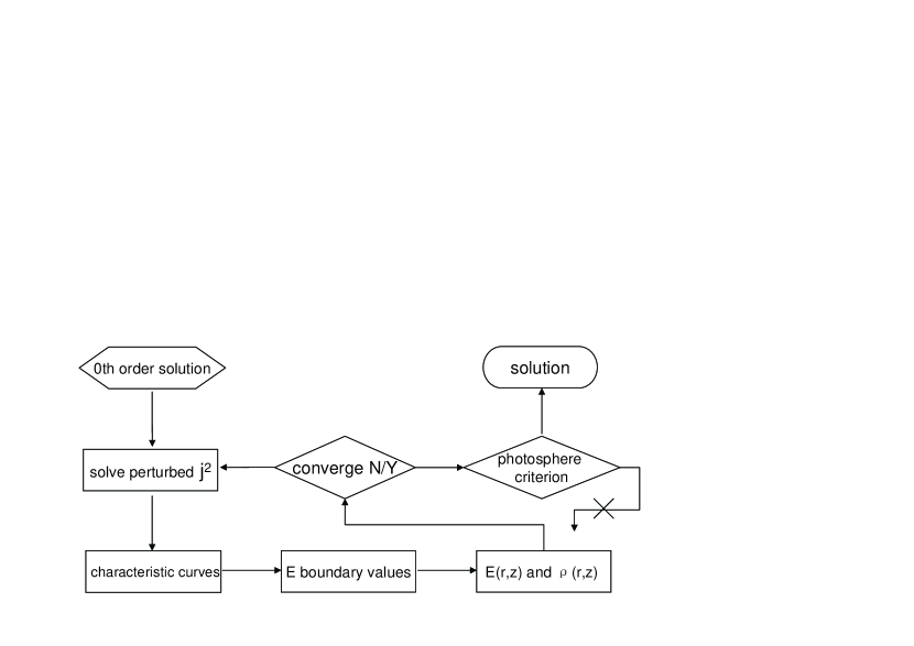
Figure 1: Flow chart of the numerical approach described in section 3.4.

To achieve a higher order of accuracy, we can follow the whole procedure again by substituting the lower order solutions into the complete set of partial differential equations and keep iterating. We terminate the procedure when further iterations no longer change the solution. Lastly, after the iterations have converged, we test whether the solution satisfies the photospheric boundary condition, accepting the result only if it does. A flow chart (Fig. 1) is presented to illustrate the procedure more clearly.

For all the numerical calculations, we construct an evenly spaced grid to cover the region $r_{in}\leq r\leq r_{max}$ and $0\leq z\leq z_{max}$, where $r_{max}$ and $z_{max}$ are determined by the boundary conditions. We use the sum $\sum\left|\frac{E_{(k)}-E_{(k-1)}}{E_{(k-1)}}\right|<N_{(k)}\varepsilon$ as the convergence criterion, where the sum includes only those grid points at which $E_{(k)}>0$, and $N_{(k)}$ is the number of those points. In addition to that criterion, we insist that the sum over those points should decrease monotonically as the order of the solution $k$ grows. We set $\varepsilon=10^{-2}$, but much higher relative accuracies (often $10^{-4}$) can be reached after several steps of iteration. The fact that the iterative method is strongly convergent proves the numerical approach based on the perturbative approximation is valid.

4 RESULTS AND DISCUSSION

4.1 Examples of Typical Solutions

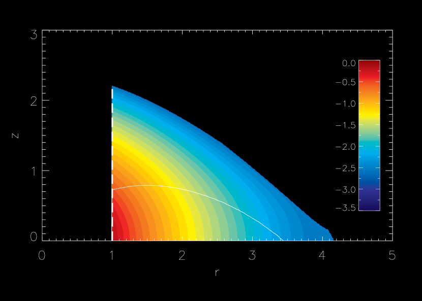
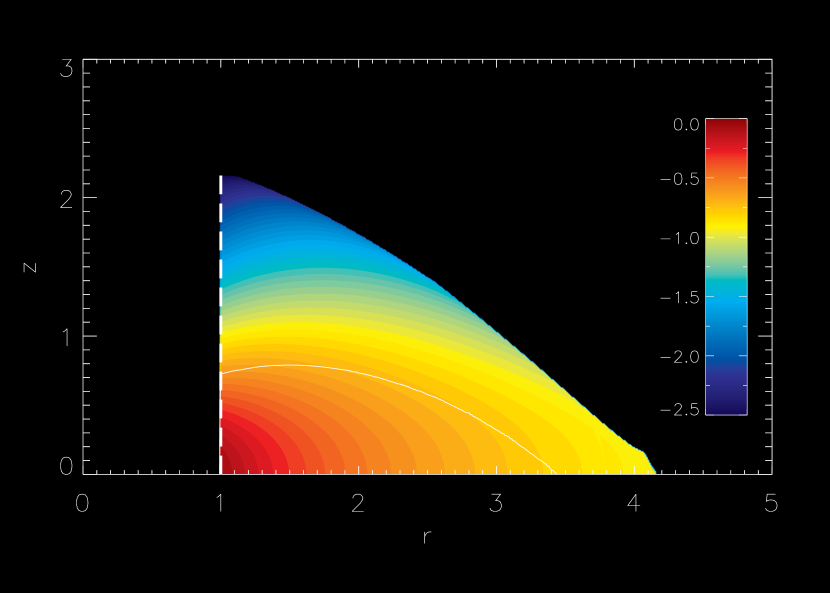
Figure 2: Solution with $j_{in}=0.5$, $\alpha=1.5$, $\tau_{*}=10$, $Q=4$, $\gamma=1.43$ and $X=0.02$. Left: Radiation energy density. Right: Matter density. In both, the scale is logarithmic, and the thin white curves show the photospheres on the top of the torus. The white dashed line marks the radius outside of which we solve the combined hydrostatic and radiation diffusion equations; it is not a physical edge.

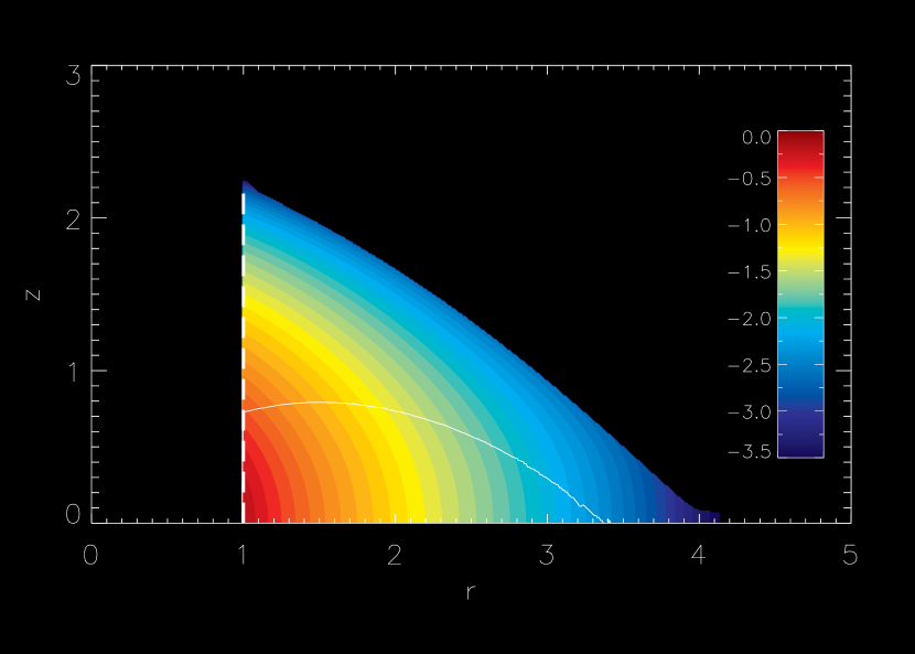
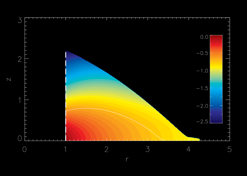
Figure 3: Solution with $j_{in}=0.5$, $\alpha=1.5$, $\tau_{*}=10$, $Q=4$, $\gamma=1.43$ and $P=2.5\times 10^{-2}$. Left: Radiation energy density. Right: Matter density. In both, the scale is logarithmic, and the thin white curves show the photospheres on the top of the torus. The white dashed line marks the radius outside of which we solve the combined hydrostatic and radiation diffusion equations; it is not a physical edge.

Let’s find the solution for typical parameters $j_{in}=0.5$, $\alpha=1.5$, $\tau_{*}=10$, $Q=4$ and $X=0.02$. Those parameters describe a torus half-supported rotationally at the inner edge, in a point mass potential, with a column density $\sim 10^{24}$ cm^-2 in the midplane, $L\sim 0.1L_{Edd}$, hard X-ray luminosity $\sim 16\%$ of the total, and $f_{c}=0.1$. The $\gamma$ determined by best fitting the boundary conditions is $\simeq 1.43$. A similar case with $X$ replaced by $P=0.025$ also requires $\gamma\simeq 1.43$; the corresponding stellar luminosity is $\sim 6\times 10^{-3}L$. These two solutions are presented in Figures 2 and 3. Like the unperturbed (no local sources) solutions shown in K07, the contours of the radiation energy density for the generalized solutions are extended upward, and the contours of the constant density are extended radially. The white curve in both figures shows the photosphere. Our diffusion approximation is validated by the fact that most of mass of the torus is within the optically thick region.

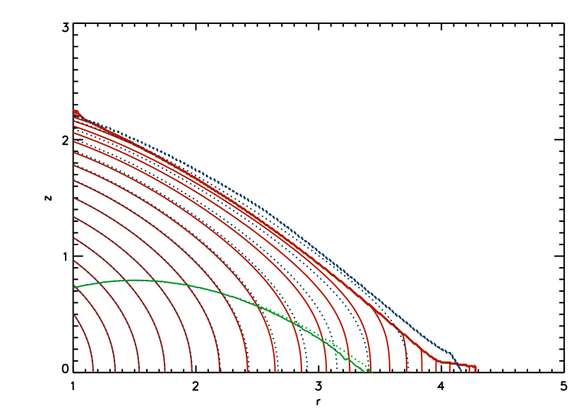
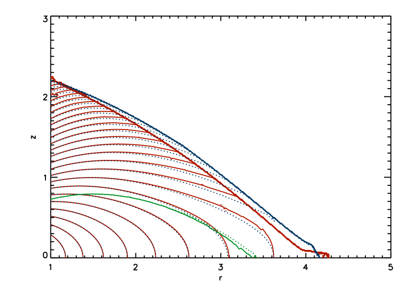
Figure 4: Comparison between two solutions which are shown in Fig. 2 and 3. Left: Radiation energy density. Right: Matter density. Red solid lines: Stellar heating case; Blue dotted lines: X-ray heating; Green solid (dotted): Photosphere for stellar heating case (X-ray heating case). Contours are in logarithmic scale with separation of $0.2$ on the left and $0.1$ on the right.

In both cases, the correction factor $f_{*}$ is almost unity, so both solutions have the same $L_{\scriptscriptstyle{UV}}$. We compare them in detail in Figure 4. The distributions of energy density and matter density are nearly the same in the optically thick zone, which suggests a rough mapping between these two local heating cases. In other words, if a solution with one internal heat source is found within the proper parameter space, a very similar solution with the other must also exist. The slight distinction at larger distance is due to the different radial and vertical dependence of their perturbations in equation 22.

4.2 Comparison With the Unperturbed

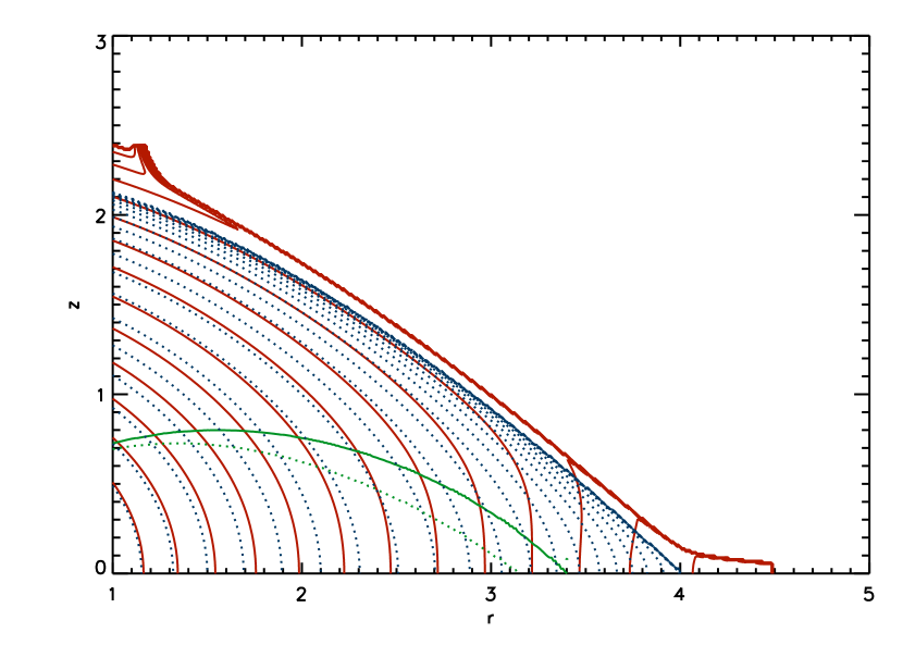
Figure 5: Comparison between unperturbed solution ($j_{in}=0.5$, $\alpha=1.5$, $\tau_{*}=10$, $Q=4.2$ and $\gamma=1.5$) and perturbed (same parameters as the unperturbed except $Q=4$ and $X=0.06$). Left: Radiation energy density. Right: Matter density. Red solid lines: Perturbed solution; Blue dotted lines: Unperturbed; Green dotted (solid): Unperturbed (perturbed) photosphere. Contours are in logarithmic scale with separation of $0.2$ on the left and $0.1$ on the right.

To better illustrate the effects of the local sources, we consider larger $X$ and $P$. Given $j_{in}=0.5$, $\alpha=1.5$, $\tau_{*}=10$, $Q=4$, and $X=0.06$ ($L_{X}/L\sim 0.38$) or $P=0.05$ ($L_{star}/L\sim 0.014$), we find that $\gamma=1.5$. Because of the similarity between the two internally-heated solutions, we need only compare one of them with the unperturbed. Here we choose X-ray heating. The correction factor $f_{*}$ for $X=0.06$ is $\sim 1.05$. Taking into account this factor, we find that an unperturbed solution with $Q\sim 4.2$ possesses the same $L_{\scriptscriptstyle{UV}}$ as that of the perturbed. $\gamma$ for this solution is $1.6$. Because there is more support at large radius with X-ray heating, the density profile becomes flatter both radially and vertically than the source-free one (Fig. 5). Meanwhile, X-ray heating also causes the energy density to decrease less rapidly away from $(r_{in},0)$ than in the unperturbed case because we are comparing at fixed $L_{\scriptscriptstyle{UV}}$ and there is now additional internally-generated flux due to the local heating.

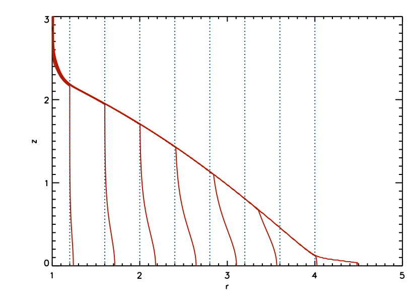
Figure 6: Distribution of $j^{2}$ for the solutions in Fig.5. Red solid lines: Perturbed. Blue dotted: Unperturbed. Contours are scaled linearly with values 0.3 to 1.0 from left to right.

Further investigation of the distribution of $j^{2}$ provides a clearer picture of the perturbed and unperturbed solutions (Fig. 6). In the interior of the torus near the inner edge, the infrared radiation pressure is large enough to balance gravity, so the presence of internal sources does not effect $j^{2}$ too much; however, at large radius, contributions from the local sources are relatively strong, while infrared flux from the inner edge diminishes. Particularly in the equatorial plane, the additional radiation support in the radial direction reduces the need for rotational support. As a consequence, the radial gradient of $j^{2}$ becomes shallower than in the case without local heating.

4.3 Exploring Parameter Space

Holding $X$ or $P$ fixed, the allowed solutions in the $Q-\gamma$ plane fall onto a track with small thickness. The thickness is due to the imprecision of the boundary condition required at the photosphere. Following the track, the parameter $\gamma$ grows as $Q$ increases. There are no solutions above or below the track. Parameters in the region below it fail the outer boundary criterion that $j=1$ at the maximum radius; those above the track do not satisfy the boundary condition at the photosphere. There is also a starting point for each track ($Q_{min},\gamma_{min}$), such that no solutions can be found with smaller $\gamma$ and $Q$. This fact, too, is an example of converged solutions that fail the boundary condition on the photosphere. In particular, when $Q<Q_{min}$, $|\mathbf{F}/cE|$ is too small, which means gravity is too weak in the torus, so that no hydrostatic balance can be achieved. The starting point moves toward larger $\gamma$ and $Q$ when $X$ or $P$ increases, while the track rises a bit due to the change of the energy density contributed from the local sources. This result is a corollary of the general picture we have presented: if UV-derived radiation support can, on its own, balance gravity, equilibrium in the presence of additional radiation force requires a smaller UV luminosity.

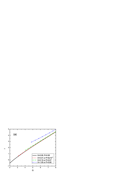
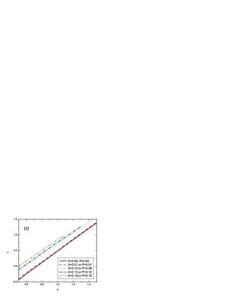
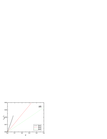
Figure 7: Solution distributions on (a) $Q-\gamma$, (b) $j_{in}-\gamma$ and (c) $\alpha-\gamma$ planes with fixed other parameters, and (d) the relationship between $P$ and the stellar luminosity. Typical values $j_{in}=0.5$, $\alpha=1.5$, $\tau_{*}=10$ and $Q=4$ are adopted if not specified.

As examples, we plot tracks with $X=0$ ($P=0$), $X=0.01$ ($P=5\times 10^{-3}$) and $X=0.10$ ($P=0.07$) in Figure 7a, which represent zero, weak and strong local sources respectively. We choose the parameters $X$ and $P$ so that the solution tracks with different local sources can be matched very well and only one curve is drawn for each set of $X$ and $P$. In K07, it was shown that $\gamma$ becomes unrealistically large for $Q\gtrsim 6$, but $Q_{min}$ could be as small as $0.1$. In Figure 7a, we see that the perturbed solutions have a smaller range of $Q$. Even for $X=0.01$ (equivalent to $P=0.005$), the minimum $Q$ permitting a solution is $\simeq 3$. In the regime of typical parameters, this range corresponds to $(L/L_{E})/\tau_{T}\sim 0.1$–0.2, with a tolerance of several. With $X\geqslant 0.1$ or $P\geqslant 0.07$, $Q$ must be greater than $4$. When we push the parameters to an unrealistic limit – $X>1.0$ ($P>0.9)$, no solutions can be found with $\gamma<3$.

We also investigate how the introduction of non-zero $X$ or $P$ alters the solution’s dependence on $j_{in}$ and $\alpha$. Like the starting points of the solution tracks in $Q-\gamma$ plane, the tracks in the $j_{in}-\gamma$ and $\alpha-\gamma$ planes possess end points. With increasing luminosity of the internal sources, for fixed $Q$, the end points move toward smaller $j_{in}$ and larger $\gamma$ (Fig. 7b), and smaller $\alpha$ and larger $\gamma$ (Fig. 7c). That means, to find dynamical balance, a stronger source in the torus demands less rotational support at the inner edge, and a less steep gravitational potential profile in the interior. As a consequence, if a torus has large $X$ or $P$, it must have a low orbital speed at $r_{in}$ and a flat potential inside. The latter might be particularly compatible with large $P$, as the flattened potential presumably reflects the contribution of stellar mass.

The last panel (d) in Figure 7 shows the roughly linear correlation between $P$ and the luminosity ratio $L_{star}/L$ as a function of $Q$, whose proportionality coefficient is determined by the integral in equation 21. Because larger $Q$ indicates less radiation support and therefore less matter density in the torus, the coefficient falls with increasing $Q$. Similar results can be found if the correlation is plotted as a function of $j_{in}$ or $\alpha$: the slopes are always positive, which means that a larger $P$ indicates a larger stellar luminosity fraction.

The characteristic optical depth $\tau_{*}$ enters in several distinct ways: with regard to the IR support due to converted UV radiation, the only effect it has independent of its presence in $Q$ is to increase the opacity, so that the photosphere rises with increasing $\tau_{*}$ is all other parameters are held constant. Otherwise, an increase in $\tau_{*}$ is equivalent to an increase in $Q$. In the perturbations, however, it has a different effect: X-ray heating is proportional to $\tau_{*}\tau_{T}X/Q$, while $Q\propto\tau_{*}$, so that in one sense the heating rate is proportional to only a single power of the column density. On the other hand, if $Q$ is held fixed, the heating rate is proportional to the square of the column density. Similarly, the stellar heating rate is $\propto\tau_{*}P/Q$, so that the combination $\tau_{*}/Q$ is independent of the column density, but this heating rate rises linearly with column density at fixed $Q$. When considering all of these scalings, it is important to note that both $\tau_{T}$ and $\tau_{*}$ are defined as characteristic optical depths ($\kappa\rho_{in}r_{in}$) rather than actual optical depths along any particular ray. For our assumption of X-ray free-streaming, the actual Thomson optical depth from the nucleus to any particular point in the torus should be $<1$. That requirement should always be satisfied if $\tau_{T}<1$; because the density falls off rapidly with increasing $r$ and increasing $|z|$, it should be satisfied in the majority of the torus volume even when $\tau_{T}\gtrsim 1$.

4.4 Comparison With Observations

One measurable diagnostic of the torus is the column density of matter along the line of sight. Although it is difficult to measure the inclination angle of the torus to the line of sight in an individual object, one can still investigate the statistical distribution of column densities to obscured AGN (Risaliti et al., 1999; Triester et al., 2004). This distribution can also be predicted by our model because the probability of a given column density is simply proportional to the solid angle associated with the polar angle producing that column. However, there is a certain level of arbitrariness in this prediction due to the guessed shape of the inner edge. Nonetheless, if we assume a vertical inner edge, the generalized solutions predict marginally wider ranges of the column densities than the unperturbed due to extra radiation pressure support. Compared with the unperturbed, although most of the solid angle is still associated with the higher column densities, the shape of that distribution tends to be flatter.

In Figure 8, we show the predicted distributions for different $X$ and $P$, keeping $L_{\scriptscriptstyle{UV}}$ fixed. The descriptions of the curves and parameters are listed in Table 1 and 2. We find that in both cases the distribution gradually extends to higher column densities when stronger local sources are present; however, the change is very small and could be unmeasurable. For large enough $X$ and $P$, the distribution curves roll over as they approach the largest column densities, an effect caused by the extended “foot” at large radius near the midplane in those solutions (e.g., the right panel of Fig. 3 and 5). Since the solution is reliable only within the photosphere, the “foot” may not be a real feature. However, it is clear that when $X,P>0$, the relative number of high column density lines of sight is diminished. For instance, the relative number of obscured AGNs per logarithm of column density reaches $\sim 1$ with $X=0.08$ at $\tau_{T}\simeq 0.4$, about half the number predicted with $X=0$. The peak in the distribution at large column density could also be reduced if the inner edge were concave near the equatorial plane, i.e., if $r_{in}(z)$ were a decreasing function of $|z|$ close to the torus midplane.

5 CONCLUSIONS

Previous work Krolik (2007) found the internal structure of radiation supported tori around AGN when they are heated only at their inner edge. In this paper, we have found generalized solutions to this problem by also taking into account two kinds of local heating sources, Compton scattering of hard X-rays and stars. Our results can be summarized in the following statements:

1. For reasonable parameters, the local sources of heating can noticeably supplement the radiation pressure support to the tori. Local heating extends the matter distribution both radially and vertically.

2. The effects of hard X-ray heating and stellar heating (at least in the Schmidt model) strongly resemble each other when their amplitudes are matched appropriately.

3. Hydrostatic equilibrium in a torus with local heating demands a smaller range of $(L/L_{E})/\tau_{T}$ than when there is none. It is $\sim 0.1$–0.2 for typical parameters. In addition, the equilibrium solutions require smaller orbital speed at the inner edge and a shallower gravitational potential inside.

4. The local sources do little to change the predicted statistical distribution of column densities.

5. In order to achieve hydrostatic equilibrium in the torus, the angular momentum has to be redistributed in both radial and vertical directions.

Placing these formal results in context, we note that in a typical AGN we expect $X\lesssim 0.05$ and $P\lesssim 0.1$. Because their effects add, we might expect that the effective amplitude of interior heating corresponds roughly to the $X\lesssim 0.1$ case. The data displayed in Figure 7a would then imply a rather limited range of $Q$ in which hydrostatic solutions can be found, $4\lesssim Q\lesssim 6$. There are three possible conclusions that can follow from this inference: The first is that there are processes that automatically tune $Q$ to lie in the permitted range. The second is that radiation pressure is so effective in supporting dusty gas against gravity that most tori are not in hydrostatic equilibrium. The third is that the numerous simplifications and approximations in our model have artificially narrowed the range of parameters permitting equilibria. We discuss them in this order.

The central parameter combination controlling $Q$ is $(L/L_{E})/\tau_{T}$, for which the range corresponding to $Q\simeq 4$–6 is $\simeq 0.1$–0.15. The actual range of $L/L_{E}$ in AGN is not, at present well-known. Moreover, most AGN mass estimates done hitherto rely on the assumption that radiation forces are unimportant compared to gravity. This is as true for those based on maser kinematics (Gallimore et al., 1996; Greenhill et al., 1997; Vlemmings et al., 2007; Kondratko, 2007) as for those based on broad emission line widths and photoionization model-estimated lengthscales (McLure & Dunlop, 2004; Kollmeier et al., 2006). It is the thrust of this paper, of course, that the dynamics of the molecular gas in which the masers are located might be substantially influenced by radiation forces. In any event, the general conclusion of these studies is that $0.1\lesssim L/L_{E}\lesssim 1$, although McLure & Dunlop (2004) might stretch the lower end of the range to $\simeq 0.03$. Estimates of the characteristic Thomson depth $\tau_{T}$ are even harder to make, but the fact that a significant fraction of all type 2 AGN appear to have column densities for which $\tau_{T}>1$ (Risaliti et al., 1999; Ueda et al., 2007; Martinez-Sansigre et al., 2007) suggests that $\tau_{T}\sim 1$, but with an unknown population dispersion, might be reasonable.

Remarkably, given both the uncertainty in the observational estimates and the extremely simplified nature of the model presented here, the nominal range of $Q$ predicted by our model agrees well with the range selected by observations if $\tau_{T}\sim 1$. Correcting the observational range of $L/L_{E}$ for a possible systematic error due to the neglect of radiation forces would tend to move it to somewhat smaller values, which would, if anything, improve the match. However, even if the intrinsic breadth of the $L/L_{E}$ distribution is as little as $\sim 4$ (as advocated by Kollmeier et al. (2006)), further tuning would be required if we take seriously the narrowness of our favored range for $Q$. One might imagine, for example, that $\tau_{T}$ adjusts in such a way as to put this ratio into the range permitting equilibrium (it is hard to see how, on the dynamical timescale of the torus, the Eddington ratio itself can be altered). While this might be possible, invoking such an effect begs the question of its mechanism: What causes the optical depth scale to change in precisely the way necessary to tune $Q$ to a value permitting equilibrium? There might also be some partial loosening of the constraints due to variations in $h$. Smaller $h$ at fixed $Q$ would imply larger $(L/L_{E})/\tau_{T}$, but also larger volumetric heating rates.

On the other hand, failure of hydrostatic equilibrium due to excess radiation pressure raises other problems. If the radiation support is too large to be balanced, accretion fuel would be blown away, which might eventually lead to a reduction in $L/L_{E}$ and the possible restoration, at least temporarily, of hydrostatic balance. However, there is a timescale mismatch problem: the mass-loss due to radiation occurs on a dynamical timescale (i.e., the orbital period), whereas inflow occurs much more slowly because it requires angular momentum transport. For this reason, readjustment of $L/L_{E}$ due to the expulsion of accretion fuel would be considerably slower than the fuel loss itself. For the same reason, resupply of the torus would be equally slow compared to the loss of torus material. Thus, a full-blown wind from the torus would lead to a long-lived state in which the nucleus continues to operate, but the torus is so depleted that there would be little obscuration.

The difficulties posed by lack of dynamical equilibrium in the torus can be made clearer by an explicit estimate of the associated mass-loss rate. Without knowing the dynamics of the outflow, we can roughly estimate the typical total mass outflow rate $\dot{M}_{out}$ by assuming that the escape speed is of the order of the local orbital speed and the outflow is isotropic. Under these assumptions, $\dot{M}_{out}\sim M_{torus}\Omega\sim 80\tau_{T}\,r_{1}^{1/2}M_{7}^{1/2}M_{\odot}~{}\textrm{yr}^{-1}$, where the numerical value of $M_{torus}$ comes from our fiducial model, $r_{1}=r_{in}/(1~{}\textrm{pc})$, and $M_{7}=M_{\scriptscriptstyle{BH}}/(107M_{\odot})$. The accretion process of the black hole must then be very wasteful, as the accretion rate required to fuel the nucleus is only $\sim 0.3(L/L_{E})M_{7}(\eta/0.1)^{-1}M_{\odot}$ yr^-1, where $\eta$ is the usual radiative efficiency in rest-mass units. Indeed, it is even quite wasteful by the standards of the mass-loss rate that might be estimated on the basis of warm absorber column densities, $\sim 1M_{7}^{1/2}r_{w,pc}^{1/2}N_{23}M_{\odot}$ yr^-1, where $r_{w,pc}$ is the characteristic radius of the warm absorber outflow in parsecs and its column density is $N_{23}$ in units of $10^{23}$ H cm^-2. Moreover, as remarked in the previous paragraph, it is hard to see how such a large outflow rate could be maintained from the outside. Estimating the resupply rate in conventional $\alpha$-model terms, we find $\dot{M}_{in}\sim 8\tau_{T}r_{1}^{1/2}M_{7}^{1/2}\alpha_{0.1}(h/r)^{2}M_{\odot}~{}\textrm{yr}^{-1}$, where $h/r$ is the ratio of the scale height to the radius, and $\alpha_{0.1}=\alpha/0.1$.

Lastly, we consider the possibility that a more careful or complete calculation might lead to more precise agreement with the observed range of $L/L_{E}$ (and $\tau_{T}$, when that is better measured). There are several improvements to our calculation that might well improve its quantitative accuracy: replacing a single averaged opacity with one that depends on frequency and substituting genuine transfer for the diffusion approximation are two that come immediately to mind. In addition, there is the intriguing possibility that a radiation-driven outflow (or possibly even a radiation-supported equilibrium) might be unstable to short-wavelength compressive fluctuations, i.e., clumping. Such a result may also be attractive for other reasons (Krolik & Begelman, 1988; Nenkova et al., 2002). If the clumping is strong enough to reduce the effective IR optical depth of the torus to $\lesssim h$, the radiation force would be diminished. This process might then be self-limiting, as the radiation dynamics responsible for clumping in the first place would likewise be weakened. Exploring these possibilities is, of course, an enterprise we must leave for future work.

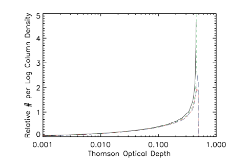
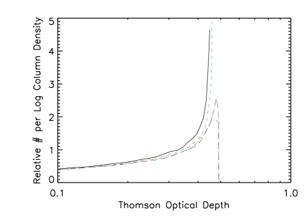
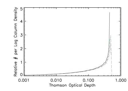
Figure 8: Predicted column density distribution for solutions with $j_{in}=0.5$, $\alpha=1.5$, $\tau_{*}=10$, $\tau_{T}=0.5$, and fixed $L_{\scriptscriptstyle{UV}}$. Left: X-ray heating case (top); Stellar heating (bottom). Right: Enlarged sections of the left. See Table 1 and 2 for descriptions of the lines and corresponding $X/P$, $Q$ and $\gamma$.

Table 1: Parameters in top two panels in Fig. 8

Line Color	Line Style	$X$	$Q$	$\gamma$
Black	Solid	0.0	4.35	1.68
Green	Dashed	0.02	4.26	1.63
Red	Dash-Dot	0.06	4.10	1.57
Blue	Long-Dashes	0.08	4.0	1.53

Table 2: Parameters in bottom two panels in Fig. 8

Line Color	Line Style	P	$Q$	$\gamma$
Black	Solid	0.0	4.35	1.68
Green	Dashed	0.02	4.25	1.63
Red	Dash-Dot	0.05	4.10	1.55
Blue	Long-Dashes	0.07	4.0	1.51

References

- Barthel (1989) Barthel, P. 1989,ApJ, 336,606
- Beckmann et al. (2006) Beckmann, V., Gehrels, N., Shrader, C.R., & Soldi, S. 2006, ApJ, 638, 642
- Chang et al. (2007) Chang, P., Quataert, E., & Murray, N. 2007, ApJ, 662, 94
- Davies et al. (2007) Davies, R.I. et al. 2007, ApJ, in presss(astro-ph/07041374)
- di Serego Alighieri et.al. (1994) di Serego Alighieri, S., Cimatti, A., & Fosbury, R.A.E. 1994, ApJ, 431, 123
- Efstathiou & Rowan-Robinson (1995) Efstathiou, A., & Rowan-Robinson,M. 1995, MNRAS, 273, 649
- Gallimore et al. (1996) Gallimore, J.F., Baum, S.A., O’Dea, C.P., Brinks, E. & Pedlar, A. 1996, ApJ, 462, 740
- Granato et al. (1997) Granato, G.L., Danese, L., & Franceschini, A. 1997, ApJ, 486, 147
- Greenhill et al. (1997) Greenhill, L.J., Moran, J.M. & Herrnstein, J.R. 1997, ApJLetts, 481, L23
- Hao, L. et al. (2005) Hao, L. et al. 2005, AJ, 2005, 129, 1795
- Jaffe et al. (2004) Jaffe, W. et al. 2004, Nature, 429, 47
- Kennicutt (1998) Kennicutt, Robert C.,Jr. 1998, ApJ, 498, 541
- Kollmeier et al. (2006) Kollmeier, J.A. et al. 2006, ApJ, 648, 128
- Kondratko (2007) Kondratko, P.T. 2007, unpublished Harvard Ph.D. thesis
- Königl & Kartje (1994) Königl, A., & Kartje, J.F. 1994, ApJ, 434, 446
- Krolik & Begelman (1988) Krolik, J.H., & Begelman, M.C. 1988, ApJ, 329, 702
- Krolik (1999) Krolik, J.H. 1999, Active Galactic Nuclei: From the Central Black Hole to the Galactic Environment, Jeremiah P. Ostriker and David N. Spergel, eds., (Princeton: New Jersey) 245
- Krolik (2007) Krolik, J.H. 2007, ApJ, 661, 52
- Marconi et al. (2004) Marconi, A. et al. 2004, MNRAS, 351, 169
- Martinez-Sansigre et al. (2007) Martinez-Sansigre, A. et al. 2007, MNRAS, 379, L6
- McLure & Dunlop (2004) McLure, R.J. & Dunlop, J.S. 2004, MNRAS, 352, 1390
- Nenkova et al. (2002) Nenkova, M., Ivezi, ., & Elitzur, M. 2002, ApJL, 570, L9
- Pier & Krolik (1992a) Pier, E.A., & Krolik, J.H. 1992a, ApJ, 399, L23
- Pier & Krolik (1992b) Pier, E.A., & Krolik, J.H. 1992b, ApJ, 401, 99
- Risaliti et al. (1999) Risaliti, D., Maiolino, R., & Salvati, M. 1999, ApJ, 522, 157
- Semenov et al. (2003) Semenov, D. et al. 2003, A&A, 410, 611
- Thompson et al. (2005) Thompson, T., Quataert, E., & Murray, N. 2005, ApJ, 630, 167
- Tozzi et al. (2006) Tozzi, R. et al. 2006, A&A, 451, 457
- Triester et al. (2004) Triester, E et al. 2004, ApJ, 616, 123
- Ueda et al. (2007) Ueda, Y. et al. 2007, ApJ, 664, 79
- Vlemmings et al. (2007) Vlemmings, W.H.T., Bignall, H.E., & Diamond, P.J. 2007, ApJ, 656, 198
- Zakamska et al. (2005) Zakamska, N. et al. 2005, AJ, 129, 1212