Temperature dependent magnetization dynamics of magnetic nanoparticles

Abstract

Recent experimental and theoretical studies show that the switching behavior of magnetic nanoparticles can be well controlled by external time-dependent magnetic fields. In this work, we inspect theoretically the influence of the temperature and the magnetic anisotropy on the spin-dynamics and the switching properties of single domain magnetic nanoparticles (Stoner-particles). Our theoretical tools are the Landau-Lifshitz-Gilbert equation extended as to deal with finite temperatures within a Langevine framework. Physical quantities of interest are the minimum field amplitudes required for switching and the corresponding reversal times of the nanoparticle’s magnetic moment. In particular, we contrast the cases of static and time-dependent external fields and analyze the influence of damping for a uniaxial and a cubic anisotropy.

1 Introduction

In recent years, there has been a surge of research activities focused on the spin dynamics and the switching behavior of magnetic nanoparticles [1]. These studies are driven by potential applications in mass-storage media and fast magneto-electronic devices. In principle, various techniques are currently available for controlling or reversing the magnetization of a nanoparticle. To name but a few, the magnetization can be reversed by a short laser pulse [2], a spin-polarized electric current [3, 4] or an alternating magnetic field [5, 6, 7, 8, 9, 10, 11, 12, 13]. Recently [6], it has been shown for a uniaxial anisotropy that the utilization of a weak time-dependent magnetic field achieves a magnetization reversal faster than in the case of a static magnetic field. For this case [6], however, the influence of the temperature and the different types of anisotropy on the various dependencies of the reversal process have not been addressed. These issues, which are the topic of this present work, are of great importance since, e.g. thermal activation affects decisively the stability of the magnetization, in particular when approaching the superparamagnetic limit, which restricts the density of data storage [14]. Here we study the possibility of fast switching at finite temperature with weak external fields. We consider magnetic nanoparticles with an appropriate size as to display a long-range magnetic order and to be in a single domain remanent state (Stoner-particles). Uniaxial and cubic anisotropies are considered and shown to decisively influence the switching dynamics. Numerical results are presented and analyzed for iron-platinum nanoparticles. In principle, the inclusion of finite temperatures in spin-dynamics studies is well-established (cf. [19, 20, 23, 15, 16, 1] and references therein) and will be followed here by treating finite temperatures on the level of Langevine dynamics. For the analysis of switching behaviour the Stoner and Wohlfarth model (SW) [17] is often employed. SW investigated the energetically metastable and stable position of the magnetization of a single domain particle with uniaxial anisotropy in the presence of an external magnetic field. They showed that the minimum static magnetic field (generally referred to as the Stoner-Wohlfarth (SW) field or limit) needed to coherently reverse the magnetization is dependent on the direction of the applied field with respect to the easy axis. This dependence is described by the so-called Stoner-Wohlfarth astroid. The SW findings rely, however, on a static model at zero temperature. Application of a time-dependent magnetic field reduces the required minimum switching field amplitude below the SW limit [6]. It was, however, not yet clear how finite temperatures will affect these findings. To clarify this point, we utilize an extension of the Landau-Lifshitz-Gilbert equation [18] including finite temperatures on the level of Langevine dynamics [19, 20, 23]. Our analysis shows the reversal time to be strongly dependent on the damping, the temperature and the type of anisotropy. These dependencies are also exhibited to a lesser extent by the critical reversal fields. The paper is organized as follows: next section 2 presents details of the numerical scheme and the notations whereas section 3 shows numerical results and analysis for Fe₅₀Pt₅₀ and Fe₇₀Pt₃₀ nanoparticles. We then conclude with a brief summary.

2 Theoretical model

In what follows we focus on systems with large spins such that their magnetic dynamics can be described by the classical motion of a unit vector ${\boldsymbol{S}}$ directed along the particle’s magnetization ${\boldsymbol{\mu}}$, i.e. ${\boldsymbol{S}}={\boldsymbol{\mu}}/\mu_{S}$ and $\mu_{S}$ is the particle’s magnetic moment at saturation. The energetics of the system is given by

$$\mathcal{H}\,=\mathcal{H}_{A}+\mathcal{H}_{F}.$$ (1)

where $\mathcal{H}_{A}$ ($\mathcal{H}_{F}$) stands for the anisotropy (Zeeman energy) contribution. Furthermore, the anisotropy contribution is expressed as $\mathcal{H}_{A}=-Df({\boldsymbol{S}})$ with $D$ being the anisotropy constant. Explicit form of $f({\boldsymbol{S}})$ is provided below. The magnetization dynamics, i.e. the equation of motion for ${\boldsymbol{S}}$, is governed by the Landau-Lifshitz-Gilbert (LLG) equation [18]

$$\frac{\partial{{\boldsymbol{S}}}}{\partial t}\,=\,-\,\frac{\gamma}{(1+\alpha^{2})}{{\boldsymbol{S}}}\times\Big{[}{{\boldsymbol{B}}_{e}}(t)\,+\,\alpha\big{(}{{\boldsymbol{S}}}\times{{\boldsymbol{B}}_{e}}(t)\big{)}\Big{]}.$$ (2)

Here we introduced the effective field ${\mathbf{B}}_{e}(t)=-1/(\mu_{S})\partial\mathcal{H}/\partial{\mathbf{S}}$ which contains the external magnetic field and the maximum anisotropy field for the uniaxial anisotropy $B_{A}=2D/\mu_{S}$. $\gamma$ is the gyromagnetic ratio and $\alpha$ is the Gilbert damping parameter. The temperature fluctuations will be described on the level of the Langevine dynamics [19]. This means, a time-dependent thermal noise ${\boldsymbol{\zeta}}(t)$ adds to the effective field ${\mathbf{B}}_{e}(t)$ [19]. ${\boldsymbol{\zeta}}(t)$ is a Gaussian distributed white noise with zero mean and vanishing time correlator

$$\quad\langle\zeta_{i}(t^{\prime})\zeta_{j}(t)\rangle=\frac{2\alpha k_{B}T}{\mu_{s}\gamma}\,\delta_{i,j}\,\delta(t-t^{\prime}).$$ (3)

$i,j$ are Cartesian components, $T$ is the temperature and $k_{B}$ is the Boltzmann constant. It is convenient to express the LLG in the reduced units

$$b=\frac{B_{e}}{B_{A}},\quad\tau=\omega_{a}t,\quad\omega_{a}=\gamma B_{A}.$$ (4)

The LLG equation reads then

$$\frac{\partial{{\boldsymbol{S}}}}{\partial\tau}=\,-\,\frac{1}{(1+\alpha^{2})}{{\boldsymbol{S}}}\times\Big{[}{{\boldsymbol{b}}}(\tau)\,+\,\alpha\big{(}{{\boldsymbol{S}}}\times{{\boldsymbol{b}}}(\tau)\big{)}\Big{]},$$ (5)

where the effective field is now given explicitly by

$${{\boldsymbol{b}}}(\tau)=-\frac{1}{\mu_{S}B_{A}}\frac{\partial\mathcal{H}}{\partial{\boldsymbol{S}}}+{{\boldsymbol{\Theta}}}(\tau)$$ (6)

with

$$\quad\langle\Theta_{i}(\tau^{\prime})\Theta_{j}(\tau)\rangle=\epsilon\,\delta_{i,j}\delta(\tau-\tau^{\prime});\>\>\epsilon\,=\frac{2\alpha k_{B}T}{\mu_{s}B_{A}}.$$ (7)

The reduced units are independent of the damping parameter $\alpha$. In the following sections we use extensively the parameter

$$q=\frac{k_{B}T}{D}.$$ (8)

$q$ is a measure for the thermal energy in terms of the anisotropy energy. And $d=D/(\mu_{S}B_{A})$ expresses the anisotropy constant in units of a maximum anisotropy energy for the uniaxial anisotropy and is always $1/2$. The stochastic LLG equation (5) in reduced units (4) is solved numerically using the Heun method which converges in quadratic mean to the solution of the LLG equation when interpreted in the sense of Stratonovich [20]. For each type of anisotropy we choose the time step $\Delta\tau$ to be one thousandth part of the corresponding period of oscillations. The values of the time interval in not reduced units for uniaxial and cubic anisotropies are $\Delta t_{ua}=4.61\cdot 10^{-15}\,s$ and $\Delta t_{ca}=64.90\cdot 10^{-15}\,s$, respectively, providing us thus with correlation times on the femtosecond time scale. The reason for the choice of such small time intervals is given in [19], where it is argued that the spectrum of thermal-agitation forces may be considered as white up to a frequency of order $k_{B}T/h$ with $h$ being the Planck constant. This value corresponds to $10^{-13}\,s$ for room temperature. The total scale of time is limited by a thousand of such periods. Hence, we deal with around one million iteration steps for a switching process. Details of realization of this numerical scheme could be found in references [21, 22, 20]. We note by passing, that attempts have been made to obtain, under certain limitations, analytical results for finite-temperature spin dynamics using the Fokker-Planck equation (cf. [15, 16] and references therein). For the general case discussed here one has however to resort to fully numerical approaches.

3 Results and interpretations

We consider a magnetic nanoparticle in a single domain remanent state (Stoner-particle) with an effective anisotropy whose origin can be magnetocrystalline, magnetoelastic and surface anisotropy. We assume the nanoparticle to have a spherical form, neglecting thus the shape anisotropy contributions. In the absence of external fields, thermal fluctuations may still drive the system out of equilibrium. Hence, the stability of the system as the temperature increases becomes an important issue. The time $t$ at which the magnetization of the system overcomes the energy barrier due to the thermal activation, also called the escape time, is given by the Arrhenius law

$$t=t_{0}e^{\frac{D}{k_{B}T}},$$ (9)

where the exponent is the ratio of the anisotropy to the thermal energy. The coefficient $t_{0}$ may be inferred when $D\gg k_{B}T$ and for high damping [19] (see [25] for a critical discussion)

$$t_{0}=\frac{1+\alpha}{\alpha\gamma}\frac{\pi\mu_{S}}{2D}\sqrt{\frac{k_{B}T}{D}}.$$ (10)

Here we focus on two different types of iron-platinum-nanoparticles: The compound Fe₅₀Pt₅₀ which has a uniaxial anisotropy [26, 27], whereas the system Fe₇₀Pt₃₀ possesses a cubic anisotropy [24]. Furthermore, the temperature dependence will be studied by varying $q$ (cf. eq.(8)).
For Fe₅₀Pt₅₀ the important parameters for simulations are the diameter of the nanoparticles $6.3\,nm$, the strength of the anisotropy $K_{u}=6\cdot 10^{6}J/m^{3}$, the magnetic moment per particle $\mu_{p}=21518\cdot\mu_{B}$ and the Curie-temperature $T_{c}=710K$ [26, 27]. The relation between $K_{u}$ and $D_{u}$ is $D_{u}=K_{u}V_{u}$, where $V_{u}$ is the volume of Fe₅₀Pt₅₀ nanoparticles. In the calculations for Fe₅₀Pt₅₀ nanoparticles the following $q$ values were chosen: $q_{1}=0.001$, $q_{2}=0.005$ or $q_{3}=0.01$ which correspond to the real temperatures $56K$, $280K$ or $560K$, respectively (these temperatures are below the blocking temperature). The corresponding escape times are $t_{q_{1}}\approx 2\cdot 10^{217}s$, $t_{q_{2}}\approx 10^{75}s$ and $t_{q_{3}}\approx 7\cdot 10^{31}s$, respectively. In some cases we also show the results for an additional temperature $q_{01}=0.0001$ with the corresponding real temperature to be equal to $5K$. The corresponding escape time for this is $t_{q_{01}}\approx 10^{4300}s$. These times should be compared with the measurement period which is about $t_{m}\approx 5\;ns$, endorsing thus the stability of the system during the measurements.
For Fe₇₀Pt₃₀ the parameters are as follows: The diameter of the nanoparticles $2.3\,nm$, the strength of the anisotropy $K_{c}=8\cdot 10^{5}J/m^{3}$, the magnetic moment per particle $\mu_{p}=2000\cdot\mu_{B}$, the Curie-temperature is $T_{c}=420K$ [24], and $D_{c}=K_{c}V_{c}$ ($V_{c}$ is the volume.) For Fe₇₀Pt₃₀ nanoparticles the values of $q$ we choose in the simulations are $q_{4}=0.01$, $q_{5}=0.03$ or $q_{6}=0.06$ which means that the temperature is respectively $0.3K$, $0.9K$ or $1.9K$. The escape times are $t_{q_{4}}\approx 10^{34}s$, $t_{q_{5}}\approx 2\cdot 10^{5}s$ and $t_{q_{6}}\approx 2\cdot 10^{-2}s$, respectively. Here we also choose an intermediate value $q_{04}=0.001$ and the real temperature $0.03K$ with the corresponding escape time to be equal to $t_{q_{04}}\approx 10^{430}s$. The measurement period is the same, namely about $5\,ns$. All values of the escape times were given for $\alpha=0.1$.
Central to this study are two issues: The critical magnetic field and the corresponding reversal time. The critical magnetic field we define as the minimum field amplitude needed to completely reverse the magnetization. The reversal time is the corresponding time for this process. In contrast, in other studies [6] the reversal time is defined as the time needed for the magnetization to switch from the initial position to the position $S_{z}=0$, our reversal time is the time at which the magnetization reaches the very proximity of the antiparallel state (Fig. 1). The difference in the definition is in so far important as the magnetization position $S_{z}=0$ at finite temperatures is not stabile so it may switch back to the initial state due to thermal fluctuations and hence the target state is never reached.

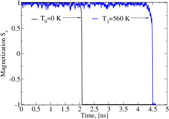
Figure 1: (Color online) Magnetization reversal of a nanoparticle when a static field is applied at zero Kelvin ($q_{0}=0$, black) and at reduced temperature $q_{3}=0.01\equiv 560K$ (blue). The strengths of the fields in the dimensionless units (4) and (8) are $b=1.01$ and $b=0.74$, respectively. The damping parameter is $\alpha=0.1$. The start position of the magnetization is given by the initial angle $\theta_{0}=\pi/360$ between the easy axis and the magnetization vector.

3.1 Nanoparticles having uniaxial anisotropy: Fe₅₀Pt₅₀

A Fe₅₀Pt₅₀ magnetic nanoparticle has a uniaxial anisotropy whose direction defines the $z$ direction. The magnetization direction ${\boldsymbol{S}}$ is specified by the azimuthal angle $\phi$ and the polar angle $\theta$ with respect to $z$. In the presence of an external field ${\boldsymbol{b}}$ applied at an arbitrarily chosen direction, the energy of the system in dimensionless units derives from

$$\tilde{\mathcal{H}}\,=-d\cos^{2}\theta-{\boldsymbol{S}}\cdot{\boldsymbol{b}}.$$ (11)

The initial state of the magnetization is chosen to be close to $S_{z}=+1$ and we aim at the target state $S_{z}=-1$.

3.1.1 Static field

For an external static magnetic field applied antiparallel to the $z$ direction (${\boldsymbol{b}}=-b{\boldsymbol{e}}_{z}$) eq.(11) becomes

$$\tilde{\mathcal{H}}\,=-d\cos^{2}\theta+b\cos\theta.$$ (12)

To determine the critical field magnitude needed for the magnetization reversal we proceed as follows (cf. Fig. 1): At first, the external field is increased in small steps. When the magnetization reversal is achieved the corresponding values of the critical field versus the damping parameter $\alpha$ are plotted as shown in the inset of Fig. 3. The reversal times corresponding to the critical static field amplitudes of Fig. 3 are plotted versus damping in Fig. 4.
In the Stoner-Wohlfarth (static) model the mechanism of magnetization reversal is not due to damping. It is rather caused by a change of the energy profile in the presence of the field. The curves displayed on the energy surface in Fig. 2 mark the magnetization motion in the $E$($\theta$,$\phi$) landscape. The magnetization initiates from $\phi_{0}=0$ and $\theta_{0}$ and ends up at $\theta=\pi$. As clearly can be seen from the figure, reversal is only possible if the initial state is energetically higher than the target state. This ”low damping” reversal is, however, quite slow, which will be quantified more below. For the reversal at $T=0$, the SW-model predicts a minimum static field strength, namely $b_{cr}=B/B_{A}=1$ (the dashed line in Fig. 3 ).
This minimum field measured with respect to the anisotropy field strength does not depend on the damping parameter $\alpha$, provided the measuring time is infinite. For $T>0$ the simulations were averaged over 500 cycles with the result shown in Fig. 3. The one-cycle data are shown in the inset. Fig. 3 evidences that with increasing temperature thermal fluctuations assist a weak magnetic field as to reverse the magnetization. Furthermore, the required critical field is increased slightly at very large and strongly at very small damping with the minimum critical field being at $\alpha\approx 1.0$. The reason for this behavior is that for low damping the second term of equation (2) is much smaller than the first one, meaning that the system exhibits a weak relaxation. In the absence of damping, higher fields are necessary to switch the magnetization. For high $\alpha$, both terms in equation (2) become small (compared to a low-damping case) leading to a stiff magnetization and hence higher fields are needed to drive the magnetization. For moderate damping, we observe a minimum of switching fields which is due to an optimal interplay between precessional and damping terms. Obviously, finite temperatures do not influence this general trend.

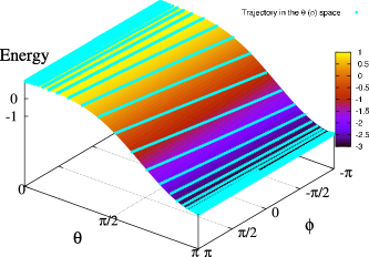
Figure 2: (Color online) The trajectories of the magnetization unit vector parameterized by the angles $\theta$ and $\phi$ at zero temperature. Other parameters are as in Fig. 1 for $q_{0}$.

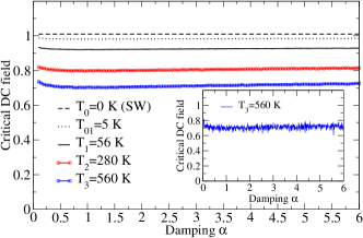
Figure 3: (Color online) Critical static field amplitudes vs. the damping parameters for different temperatures averaged over 500 times. Inset shows not averaged data for $q_{3}=0.01\equiv 560K$.

For the case of $q_{0}=0$, the Landau-Lifshitz-Gilbert equation of motion can be solved analytically in spherical coordinates. The details of the solution can be found in Ref. [20] (eq. (A1)-(A8)). The final result of the solution in this reference differs, however, from the one given here due to to different geometries in these systems. In contrast to our alignment of the magnetization and the external field, the static field in Ref. [20] is applied parallel to the initial position of the magnetization. For the solution, we assume that the magnetization starts at $\theta=\theta_{0}=\pi/360$ and arrives at $\theta=\pi$. Note, that the expression $\theta\neq 0$ is important only for zero Kelvin since the switching is not possible if the magnetization starts at $\theta_{0}=0$ (the vector product in equation (2) vanishes). The reversal time in the SW-limit is then given by

$$t_{rev}=g(\theta_{0},b)\frac{1+\alpha^{2}}{\alpha},$$ (13)

where $g$ is defined as

$$g(\theta_{0},b)=\frac{\mu_{S}}{2\gamma D}\frac{1}{b^{2}-1}\ln\left(\frac{tg(\theta/2)^{b}\sin\theta}{b-\cos\theta}\right)\Big{|}^{\pi}_{\theta_{0}}.$$ (14)

From this relation we infer that switching is possible only if the applied field is larger than the anisotropy field and the reversal time decreases with increasing $b$. This conclusion is independent of the Stoner-Wohlfarth model and follows directly from the solution of the LLG equation. An illustration is shown by the dashed curve in Fig. 4, which was a test to compare the appropriate numerical results with the analytical one. As our aim is the study of the reversal-time dependence on the magnetic moment and on the anisotropy constant, we deem the logarithmic dependence in Eq.(14) to be weak and write

$$g(b,\mu_{S},D)\approx\frac{\mu_{S}}{\gamma}\frac{2D}{B^{2}\mu_{S}^{2}-4D^{2}}.$$ (15)

This relation indicates that an increase in the magnetic moment results in a decrease of the reversal time. The magnetic moment enters in the Zeeman energy and therefore the increase in magnetic moment is very similar to an increase in the magnetic field. An increase of the reversal time with the increasing anisotropy originates from the fact that the anisotropy constant determines the height of the potential barrier. Hence, the higher the barrier, the longer it takes for the magnetization to overcome it.
For the other temperatures the corresponding reversal times (also averaged over 500 cycles) are shown in Fig. 4. In contrast to the case $T=0$, where an appreciable dependence on damping is observed, the reversal times for finite temperatures show a weaker dependence on damping. If $\alpha\rightarrow 0$ only the precessional motion of the magnetization is possible and therefore $t_{rev}\rightarrow\infty$. At high damping the system relaxes on a time scale that is much shorter than the precession time, giving thus rise to an increase in switching times. Additionally, one can clearly observe the increase of the reversal times with increasing temperatures, even though these time remain on the nanoseconds time scale.

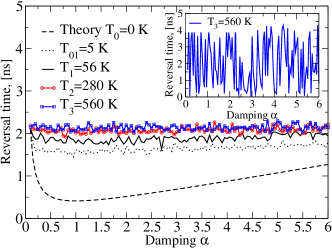
Figure 4: (Color online) Reversal times corresponding to the critical static fields in Fig. 3 vs. damping averaged over 500 cycles. Inset shows the as-calculated numerical results for $q_{3}=0.01\equiv 560K$ (one cycle).

3.1.2 Alternating field

As was shown in Ref. [6, 7, 15] theoretically and in Ref. [5] experimentally, a rotating alternating field with no static field being applied can also be used for the magnetization reversal. A circular polarized microwave field is applied perpendicularly to the anisotropy axis. Thus, the Hamiltonian might be written in form of equation (11) and the applied field is

$${\boldsymbol{b}}(t)=b_{0}\cos\omega t{\boldsymbol{e}}_{x}+b_{0}\sin\omega t{\boldsymbol{e}}_{y},$$ (16)

where $b_{0}$ is the alternating field amplitude and $\omega$ is its frequency. For a switching of the magnetization the appropriate frequency of the applied alternating field should be chosen. In Ref. [15] analytically and in [6] numerically a detailed analysis of the optimal frequency is given which is close to the precessional frequency of the system. The role of temperature and different types of anisotropy have not yet been addressed, to our knowledge.

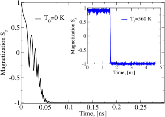
Figure 5: (Color online) Magnetization reversal in a nanoparticle using a time dependent field for $\alpha=0.1$ and at a zero temperature. The field strength and frequency in the units (4) are respectively $b_{0}=0.18$ and $\omega=\omega_{a}/1.93$. Inset shows for this case the magnetization reversal for the temperature $q_{3}=0.01\equiv 560K$ with $b_{0}=0.17$ and the same frequency.

Fig. 5 shows our calculations for the reversal process at two different temperatures. In contrast to the static case, the reversal proceeds through many oscillations on a time scale of approximately ten picoseconds. Increasing the temperature results in an increase of the reversal time.

Fig. 6 shows the trajectory of the magnetization in the E($\theta$,$\phi$) space related to the case of the alternating field application. Compared with the situation depicted in Fig. 2, the trajectory reveals a quite delicate motion of the magnetization. It is furthermore, noteworthy that the alternating field amplitudes needed for the reversal (cf. Fig. 7) are substantially lower than their static counterpart, meaning that the energy profile of the system is not completely altered by the external field.

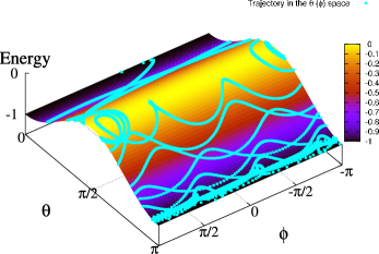
Figure 6: (Color online) Trajectories followed by magnetization as specified by $\theta$ and $\phi$ for $q_{0}=0$. Other parameters are $b_{0}=0.18$, $\alpha=0.1$ and $\omega=\omega_{a}/1.93$. Energy-profile variations due to the oscillating external field are not visible on this scale.

Fig. 7 inspects the dependence of the minimum switching field amplitude on damping. The critical fields are obtained upon averaging over 500 cycles. The SW-limit lies by $1$ on this scale. In contrast to the static case, the critical fields increase with increasing $\alpha$. In the low damping regime the critical field is smaller than in the case of a static field. This behavior can be explained qualitatively by a resonant energy-absorption mechanism when the frequencies of the applied field matches the frequency of the system. Obviously, at very low frequencies (compared to the precessional frequency) the dynamics resembles the static case.
The influence of the temperature on the minimum alternating field amplitudes is depicted in Fig. 7. With increasing temperatures, the minimum amplitudes become smaller due to an additional thermal energy pumped from the environment. The curves in this figure can be approached with two linear dependencies with different slopes for approximately $\alpha<1$ and for $\alpha>1$; for high damping it is linearly dependent on $\alpha$, more specifically it can be shown that for high damping the critical fields behave as

$$b_{cr}\approx\frac{1+\alpha^{2}}{\alpha}.$$ (17)

The proportionality coefficient contains the frequency of the alternating field and the critical angle $\theta$. The solution (17) follows from the LLG equation solved for the case when the phase of the external field follows temporally that of the magnetization, which we checked numerically to be valid.

The reversal times associated with the critical switching fields are shown in (Fig. 8). Qualitatively, we observe the same behavior as for the case of a static field. The values of the reversal times for $T=0$ are, however, significantly smaller than for the static case. For the same reason as in the static field case, an increased temperature results in an increase of the switching times.

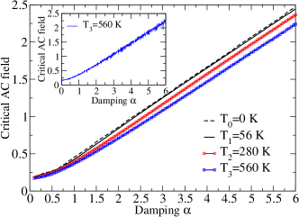
Figure 7: (Color online) Critical alternating field amplitudes vs. damping for different temperatures averaged over 500 times. Inset shows not averaged data for $q_{3}=0.01\equiv 560K$.

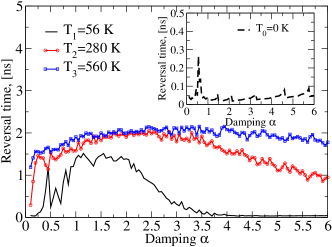
Figure 8: (Color online) The damping dependence of the reversal times corresponding to the critical field amplitudes of Fig. 7 for different temperatures. Inset shows the case of zero Kelvin.

3.2 Nanoparticles with cubic anisotropy: Fe₇₀ Pt₃₀

Now we focus on another type of the anisotropy, namely a cubic anisotropy which is supposed to be present for Fe₇₀Pt₃₀ nanoparticles [24]. The energetics of the system is then described by the functional form

$$\tilde{\mathcal{H}}\,=-d(S_{x}^{2}S_{y}^{2}+S_{y}^{2}S_{z}^{2}+S_{x}^{2}S_{z}^{2})-{\boldsymbol{S}}\cdot{\boldsymbol{b}},$$ (18)

or in spherical coordinates

$$\tilde{\mathcal{H}}\,=-d(\cos^{2}\phi\sin^{2}\phi\sin^{4}\theta+\cos^{2}\theta\sin^{2}\theta)-{\boldsymbol{S}}\cdot{\boldsymbol{b}}.$$ (19)

In contrast to the previous section, there are more local minima or in other words more stable states of the magnetization in the energy profile for the Fe₇₀Pt₃₀ nanoparticles. It can be shown that the minimum barrier that has to be overcome is $d/12$ which is twelve times smaller than that in the case of a uniaxial anisotropy. The maximal one is only $d/3$.
The magnetization of these nanoparticles is first relaxed to the initial state close to $\phi_{0}=\pi/4$ and $\theta_{0}=\arccos(1/\sqrt{3})$, whereas in the target state it is aligned antiparallel to the initial one, i. e. $\phi_{e}=3\pi/4$ and $\theta_{e}=\pi-\arccos(1/\sqrt{3})$. In order to be close to the starting state for the uniaxial anisotropy case we choose $\phi_{0}=0.2499\cdot\pi$, $\theta_{0}=0.3042\cdot\pi$.

3.2.1 Static driving field

A static field is applied antiparallel to the initial state of the magnetization, i.e.

$${\boldsymbol{b}}=-b/\sqrt{3}({\boldsymbol{e}}_{x}+{\boldsymbol{e}}_{y}+{\boldsymbol{e}}_{z}).$$ (20)

In Fig. 9 the trajectory of the magnetization in case of an applied static field is shown. Similar to the previous section the energy of the initial state lies higher than that of the target state. The magnetization rolls down the energy landscape to eventually end up by the target state. The trajectory the magnetization follows is completely different from the one for the uniaxial anisotropy. Fig. 10 supplements this scenario of the magnetization reversal by showing the time evolution of the $S_{z}$ vector. Because of the different anisotropy type, the trajectory is markedly different from the case of the uniaxial anisotropy and a static field. Here we show only the $S_{z}$ magnetization component even though the other components also have to be taken into account in order to avoid a wrong target state.
The procedure to determine the critical field amplitudes is similar to that described in the previous section. In Fig. 11 the critical fields versus the damping parameter for different temperatures are shown. For $q_{0}$, the critical field strength is smaller than $1$. This is consistent insofar as the maximum effective field for a cubic anisotropy is $\frac{2}{3}B_{A}$. In principle, the critical field turns out to be constant for all $\alpha$ but for an infinitely large measuring time. Since we set this time to be about $5$ nanoseconds, the critical fields increase for small and high damping. On the other hand, at lower temperatures smaller critical fields are sufficient for the (thermal activation-assisted) reversal process.

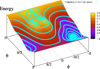
Figure 9: (Color online) Trajectories of the magnetization in the $\theta$($\phi$) space ($q_{0}=0$). In the units (4) we choose $b=0.82$ and $\alpha=0.1$.

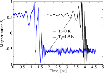
Figure 10: (Color online) Magnetization reversal of a nanoparticle when a static field $b=0.82$ is applied and for $\alpha=0.1$ at zero temperature (black). The magnetization reversal for $\alpha=0.1$, $b=0.22$ and $q_{6}=0.06\equiv 1.9K$ is shown with blue color.

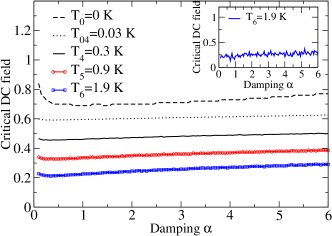
Figure 11: (Color online) Critical static field amplitudes vs. the damping parameters for different temperatures averaged over 500 times. Inset shows not averaged data for $q_{6}=0.06\equiv 1.9K$.

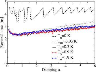
Figure 12: (Color online) Reversal times corresponding to the critical static fields of Fig. 11 vs. damping averaged over 500 times.

The behaviour of the corresponding switching times presented in Fig. 12 only supplements the fact of too low measuring time, which is chosen as $5\,ns$ for a better comparison of these results with ones for uniaxial anisotropy. Indeed, constant jumps in the reversal times for $T=0\,K$ as a function of damping can be observed. The reason why the reversal times for finite temperatures are lower is as follows: The initial state for $T=0\,K$ is chosen to be very close to equilibrium. This does not happen for finite temperatures, where the system due to thermal activation jumps out of equilibrium (cf. see Fig. 10).

3.2.2 Time-dependent external field

Here we consider the case of an alternating field that rotates in the plain perpendicularly to the initial state of the magnetization. It is possible to switch the magnetization with a field rotating in the $xy-$ plane but the field amplitudes turn out to be larger than those when the field rotates perpendicular to the initial state. For the energy this means that the field entering equation (19) reads

$${\boldsymbol{b}}(t) = (b_{0}\cos\omega_{1}t\cos\phi_{0}+b_{0}\sin\omega_{1}t\sin\phi_{0}\cos\theta_{0}){\boldsymbol{e}}_{x}$$ (21)

$$+(-b_{0}\cos\omega_{1}t\sin\phi_{0}+b_{0}\sin\omega_{1}t\cos\phi_{0}\cos\theta_{0}){\boldsymbol{e}}_{y}+(-b_{0}\sin\theta_{0}\sin\omega_{1}t){\boldsymbol{e}}_{z},$$

where $b_{0}$ is the alternating field amplitude and $\omega_{1}$ is the frequency associated with the field. This expression is derived upon a rotation of the field plane by the angles $\phi_{0}=\pi/4$ and $\theta_{0}=\arccos(1/\sqrt{3})$.
The magnetization trajectories depicted in Fig. 13 reveal two interesting features: Firstly, particularly for small damping, the energy profile changes very slightly (due to the smallness of $b_{0}$) while energy is pumped into the system during many cycles. Secondly, the system switches mostly in the vicinity of local minima to acquire eventually the target state. Fig. 14 hints on the complex character of the magnetization dynamics in this case.

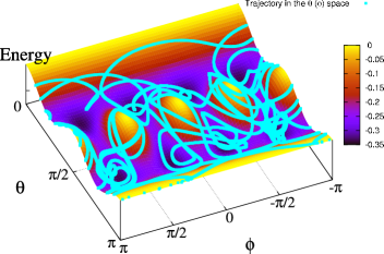
Figure 13: (Color online) Trajectories of the magnetization vector specified by the angles $\theta$ and $\phi$ at zero temperature. The chosen parameters are $b_{0}=0.055$ and $\omega=\tilde{\omega_{a}}/1.93$, where $\tilde{\omega_{a}}=2/3\omega_{a}$.

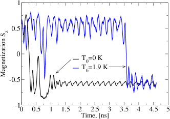
Figure 14: (Color online) Magnetization reversal in a nanoparticle using a time dependent field for $\alpha=0.1$ and $q_{0}$ (black) and for $q_{6}=0.06\equiv 1.9K$ (blue). Other parameters are as in Fig. 13.

As in the static field case with a cubic anisotropy the critical field amplitudes shown in Fig. 15 are smaller than those for a uniaxial anisotropy. Obviously, the reason is that the potential barrier associated with this anisotropy is smaller in this case, giving rise to smaller amplitudes. As before an increase in temperature leads to a decrease in the critical fields.

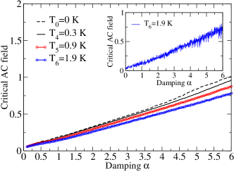
Figure 15: (Color online) Critical alternating field amplitudes vs. damping for different temperatures averaged over 500 cycles. Inset shows the single cycle data at $q_{6}=0.06\equiv 1.9K$.

The reversal times shown in Fig. 16 exhibit the same feature as in the cases for uniaxial anisotropy: With increasing temperatures the corresponding reversal times increase. A physically convincing explanation of the (numerically stable) oscillations for the reversal times is still outstanding.

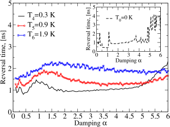
Figure 16: (Color online) The damping dependence of the reversal times corresponding to the critical fields of the Fig. 15 for different temperatures averaged over 500 runs. Inset shows the $T=0$ case.

4 Summary

In this work we studied the critical field amplitudes required for the magnetization switching of Stoner nanoparticles and derived the corresponding reversal times for static and alternating fields for two different types of anisotropies. The general trends for all examples discussed here can be summarized as follows: Firstly, increasing the temperature results in a decrease of all critical fields regardless of the anisotropy type. Anisotropy effects decline with increasing temperatures making it easier to switch the magnetization. Secondly, elevating the temperature increases the corresponding reversal times. Thirdly, the same trends are observed for different temperatures: The critical field amplitudes for a static field depend only slightly on $\alpha$, whereas the critical alternating field amplitudes exhibit a pronounced dependence on damping. In the case of a uniaxial anisotropy we find the critical alternating field amplitudes to be smaller than those for a static field, especially in the low damping regime and for finite temperatures. Compared with a static field, alternating fields lead to smaller switching times ($T=0\,K$). However, this is not the case for the cubic anisotropy. The markedly different trajectories for the two kinds of anisotropies endorse the qualitatively different magnetization dynamics. In particular, one may see that for a cubic anisotropy and for an alternating field the magnetization reversal takes place through the local minima leading to smaller amplitudes of the applied field. Generally, a cubic anisotropy is smaller than the uniaxial one giving rise to smaller slope of critical fields, i.e. smaller alternating field amplitudes.
It is useful to contrast our results with those of Ref. [15]. Our reversal times for AC-fields increase with increasing temperatures. This is not in contradiction with the findings of [15] insofar as we calculate the switching fields at first, and then deduce the corresponding reversal times. If the switching fields are kept constant while increasing the temperature [15] the corresponding reversal times decrease. We note here that experimentally known values of the damping parameter are, to our knowledge, not larger than $0.2$. The reason why we go beyond this value is twofold. Firstly, the values of damping are only well known for thin ferromagnetic films and it is not clear how to extend them to magnetic nanoparticles. For instance, in FMR experiments damping values are obtained from the widths of the corresponding curves of absorption. The curves for nanoparticles can be broader due to randomly oriented easy anisotropy axes and, hence, the values of damping could be larger than they actually are. Secondly, due to a very strong dependence of the critical AC-fields (Fig. 7, e.g.) they can even be larger than static field amplitudes. This makes the time-dependent field disadvantageous for switching in an extreme high damping regime.
Finally, as can be seen from all simulations, the corresponding reversal times are much more sensitive a quantity than their critical fields. This follows from the expression (13), where a slight change in the magnetic field $b$ leads to a sizable difference in the reversal time. This circumstance is the basis for our choice to average all the reversal times and fields over many times. This is also desirable in view of an experimental realization, for example, in FMR experiments or using a SQUID technique quantities like critical fields and their reversal times are averaged over thousands of times. The results presented in this paper are of relevance to the heat-assisted magnetic recording, e.g. using a laser source. Our calculations do not specify the source of thermal excitations but they capture the spin dynamics and switching behaviour of the system upon thermal excitations.

References

References

- [1] Spindynamics in confined magnetic structures III B. Hillebrands, A. Thiaville (Eds.) (Springer, Berlin, 2006); Spin Dynamics in Confined Magnetic Structures II B. Hillebrands, K. Ounadjela (Eds.) (Springer, Berlin, 2003); Spin dynamics in confined magnetic structures B. Hillebrands, K. Ounadjela (Eds.) (Springer, Berlin, 2001); Magnetic Nanostructures B. Aktas, L. Tagirov, F. Mikailov (Eds.), (Springer Series in Materials Science, Vol. 94) (Springer, 2007) and references therein.
- [2] M. Vomir, L. H. F. Andrade, L. Guidoni, E. Beaurepaire, and J.-Y. Bigot, Phys. Rev. Lett. 94, 237601 (2005).
- [3] J. Slonczewski, J. Magn. Magn. Mater., 159, L1, (1996).
- [4] L. Berger, Phys. Rev. B 54, 9353 (1996).
- [5] C. Thirion, W. Wernsdorfer, and D. Mailly, Nat. Mater. 2, 524 (2003).
- [6] Z. Z. Sun and X. R. Wang, Phys. Rev. B 74, 132401 (2006).
- [7] Z. Z. Sun and X. R. Wang, Phys. Rev. Lett. 97, 077205 (2006).
- [8] L. F. Zhang, C. Xu, Physics Letters A 349, 82-86 (2006).
- [9] C. Xu, P. M. Hui , Y. Q. Ma, et al., Solid State Communications 134, 625-629 (2005).
- [10] T. Moriyama, R. Cao, J. Q. Xiao, et al., Applied Physics Letters 90, 152503 (2007).
- [11] H. K. Lee, Z. M. Yuan, Journal of Applied Physics 101, 033903 (2007).
- [12] H. T. Nembach, P. M. Pimentel, S. J. Hermsdoerfer, et al., Physics Letters 90, 062503 (2007).
- [13] K. Rivkin, J. B. Ketterson, Applied Physics Letters 89, 252507 (2006).
- [14] R. W. Chantrell and K. O’Grady The Magnetic Properties of fine Particles in R. Gerber, C. D. Wright and G. Asti (Eds.), Applied Magnetism (Kluwer, Academic Pub., Dordrecht, 1994).
- [15] S. I. Denisov, T. V. Lyutyy, P. Hänggi, and K. N. Trohidou, Phys. Rev. B 74, 104406 (2006).
- [16] S. I. Denisov, T. V. Lyutyy, and P. Hänggi, Phys. Rev. Lett. 97, 227202 (2006).
- [17] E. C. Stoner and E. P. Wohlfarth, Philos. Trans. R. Soc. London, Ser A 240, 599 (1948).
- [18] L. Landau and E. Lifshitz, Phys. Z. Sowjetunion 8, 153 (1935).
- [19] W. F. Brown, Phys. Rev. 130, 1677 (1963).
- [20] J. L. Garcia-Palacios and F. Lazaro, Phys. Rev. B 58, 14937 (1998).
- [21] Algorithmen in der Quantentheorie und Statistischen Physik J. Schnakenberg (Zimmermann-Neufang, 1995).
- [22] U. Nowak, Ann. Rev. Comp. Phys. 9, 105 (2001).
- [23] K. D. Usadel, Phys. Rev. B 73, 212405 (2006).
- [24] C. Antoniak, J. Lindner, and M. Farle, Europhys. Lett. 70, 250 (2005).
- [25] I. Klik and L. Gunther, J. Stat. Phys. 60, 473 (1990).
- [26] C. Antoniak, J. Lindner, M. Spasova, D. Sudfeld, M. Acet, and M. Farle, Phys. Rev. Lett. 97, 117201 (2006).
- [27] S. Ostanin, S. S. A. Razee, J. B. Staunton, B. Ginatempo and E. Bruno, J. Appl. Phys. 93, 453 (2003).