Resummation of projectile-target multiple scatterings and parton saturation

Abstract

In the framework of a toy model which possesses the main features of QCD in the high energy limit, we conduct a numerical study of scattering amplitudes constructed from parton splittings and projectile-target multiple interactions, in a way that unitarizes the amplitudes without however explicit saturation in the wavefunction of the incoming states. This calculation is performed in two different ways. One of these formulations, the closest to field theory, involves the numerical resummation of a factorially divergent series, for which we develop appropriate numerical tools. We accurately compare the properties of the resulting amplitudes with what would be expected if saturation were explicitly included in the evolution of the states. We observe that the amplitudes have similar properties in a small but finite range of rapidity in the beginning of the evolution, as expected. Some of the features of reaction-diffusion processes are already present in that range, even when saturation is left out of the model.

I Introduction

Saturation of parton densities is a phenomenon that is expected to occur in the scattering of very fast hadrons GLR ; MQ . It is the statement that the number of partons per unit of transverse phase space in the Fock states of the incoming hadrons does not grow exponentially forever with energy (or rapidity), as would come out of a naive solution of linear evolution equations: The growth gets softer at very high energies, in such a way that the unitarity of the probabilities of scattering be preserved.

However, it seems very difficult to get saturation from a field-theoretical calculation. So far, the problem has not even been formulated properly in QCD, for it is already very challenging to identify the graphs that should be taken into account. Equations such as the Balitsky equation Balitsky:1995ub (which is in fact a hierarchy of equations) have been written down, but they do not exhibit saturation in an obvious way (if at all), and they are anyway extremely difficult to solve.

Despite these fundamental difficulties, new quantitative results could be obtained for QCD amplitudes in the saturation regime over the last few years Mueller:2004sea ; IMM . In short, they rely on an analogy with reaction-diffusion processes IMM but not on the computation of definite Feynman graphs. The obtained results do not depend on the way how partons saturate, but they seem to require that there be such saturation phenomena. So saturation was assumed rather than found in these approaches. The matching of this statistical picture with field-theory calculations has been attempted Iancu:2004iy , and has led to the statement that the Balitsky-Jalilian Marian-Iancu-McLerran-Weigert-Leonidov-Kovner (B-JIMWLK) equations Balitsky:1995ub ; JIMWLK ; Weigert:2005us were incomplete, and that they had to be supplemented with new terms. The problem was identified as follows: The Balitsky equations only contain splittings of partons, while mergings are needed in order to achieve saturation. The hope that merging rates could be obtained by boosting splitting vertices was turned down by the finding that this procedure would lead to negative probabilities MSW ; IST , which is at least inconvenient in practice MMX , if not completely meaningless.

In this paper, we go back to the original formulation of saturation by Mueller in the context of the color dipole model M1 ; M2 ; M3 , which was in fact based on the assumption that saturation of the parton densities is equivalent to unitarization of the scattering amplitudes through multiple exchanges between linearly-evolved Fock states of the incoming particles (if the rapidity is not too high). Analytical calculations have been achieved within similar approximations (see Refs. Levin1 ; Levin2 for recent progress), but the result looks always complicated in QCD and thus difficult to play with and to interpret. Numerical studies were conducted by Salam S1 ; S_MC ; MS , but at that time, there was no good theoretical understanding of the properties that scattering amplitudes should exhibit at high energy. In the light of our present knowledge of saturation, that enables us to characterize saturation by analyzing the properties of some traveling waves, we evaluate numerically, on toy models, how good this procedure is when only splittings and multiple exchanges are allowed. Another important highlight of the present work is that we are able to resum numerically the asymptotic series that can be constructed out of an expansion in the number of rescatterings, and which has the structure of the proper field-theoretical series of successive Pomeron exchanges.

Our study assumes the following standard picture of scattering in the QCD parton model (see Fig. 1): An asymptotic hadron, made of valence partons, evolves into a set of quarks and gluons spread in impact parameter space, when its rapidity is increased. The rules of splitting (and recombination when nonlinear effects are taken into account in the evolution) of the partons are fixed by the QCD Lagrangian. Two such hadrons interact with each other by exchanging, with probability of the order of $\alpha^{2}$ ($\alpha$ is the strong coupling constant), one or several gluons between the partons of similar sizes and impact parameters that are present in the wavefunctions of the two hadrons at the time of the interaction.

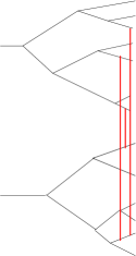
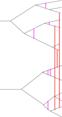
Figure 1: Sketch of the scattering of the two evolved hadrons through splittings only (left) and through splittings supplemented by nonlinear effects (here in the form of internal rescatterings; rightmost figure.) The vertical thick lines would correspond to gluon exchanges in QCD. Each of them comes with an extra power of $\alpha^{2}$ which is not enhanced by corresponding powers of the rapidity.

The outline goes as follows. In the next section (Sec. II), we introduce a model for partonic state evolution under splittings only. Sec. III is devoted to the formulation of the unitary scattering amplitudes built from these states, that we compare to cases in which saturation is included explicitly in the evolution. The numerical study of the many variants of the toy model, in different frames and within different unitarization schemes, is the object of Sec. IV. In Sec. V we present an alternative calculation, based on the numerical resummation of the asymptotic series in the number of Pomerons that are exchanged. We state our conclusions and some prospects in the last section.

II Toy model for linear parton evolution

II.1 Construction of the model

Focussing on one particular impact parameter, one may reduce the QCD problem to one transverse dimension only. It is very important to keep the dynamics in the transverse space if one wants the model to be representative of some of the physics of QCD. However, we do not aim at incorporating all aspects of QCD: We need a simple model, that is easy to formulate in a way which can be implemented in the form of a Monte-Carlo event generator. Let us assume that there be only one type of object in the theory, which could be gluons or, more accurately, color dipoles, and that the latter may be fully characterized by a single “space” variable, which represents for example their size in the transverse plane. There is in addition an evolution variable: the rapidity. So far, we have in fact just idealized the color dipole model M1 .

To further simplify the model, we discretize it both in space and in rapidity. The evolution rule is the following: When the rapidity $y$ is increased by one unit, a particle at position $i$ on the lattice may be replaced, with probability $\frac{1}{2}$, by two offspring at respective positions $i+j$ and $i-j$. For the distribution of $j$, we choose:

$$\text{Proba}(j)=\left(1-\frac{1}{e}\right)e^{-j}.$$ (1)

This rule obviously leads to an exponential increase of the number of objects on each site, which can eventually break the unitarity constraints. Nevertheless, we do not a priori specify a saturation mechanism at this level: Several options of implementing unitarity of the scattering amplitudes will be examined in the next section, and saturation, in the sense that the number of particles is prevented from exhibiting an exponential growth forever, will only be one of them.

Note that the choice of discrete transverse space and especially discrete $y$ is not very natural for a model that is meant to mimic QCD, in particular since discretizing $y$ obviously breaks boost invariance (which makes sure that the rapidity evolution can be shared arbitrarily between the two incoming hadrons without affecting the observables). However, this choice is dictated by technical reasons: We will need to be able to generate millions of events within some reasonable computer time.

Let us define the generating function for the probability of the different configurations as

$$Z(y,\{x_{k}\})=\sum_{\{n_{k}\}}\left(\prod_{k}x_{k}^{n_{k}}\right)P(y,\{n_{k}\}),$$ (2)

where $P(y,\{n_{k}\})$ is the probability of having $\cdots n_{1},\cdots,n_{k},\cdots$ particles on sites $\cdots 1,\cdots,k,\cdots$ at rapidity $y$. This function contains all information about the statistics of the particle numbers on all sites. For example, the correlator of the number of particles on sites 1 and 2 is obtained by taking two derivatives:

$$\left.\frac{\partial Z}{\partial x_{1}\partial x_{2}}\right|_{x_{k}=1}=\langle n_{1}n_{2}\rangle.$$ (3)

The generating function $Z$ obeys the evolution equation

$$Z(y+1,\{x_{k}\})=\frac{1}{2}Z(y,\{x_{k}\})\\ +\frac{1}{2}\left(1-\frac{1}{e}\right)\sum_{j=0}^{\infty}e^{-j}Z(y,\{x_{k-j}\})Z(y,\{x_{k+j}\}).$$ (4)

This equation is easily derived by considering the very first step in rapidity and with the help of the probability distribution (1). This is actually a version of what we call in QCD the Balitsky-Kovchegov (BK) equation Balitsky:1995ub ; K1 ; K2 associated to this simplified model. The physical $S$-matrix element in this framework, $S_{\text{BK}}(y,i)$, is a particular value of $Z$, obtained from the above equation by setting $x_{k\neq i}=1$ and $x_{i}=e^{-\alpha^{2}}$. The nonlinearity in Eq. (4) makes sure that $S$ be unitary. We will define the scattering amplitudes properly only in Sec. III, but before, we may summarize the main known properties of $S_{\text{BK}}$ seen as a solution of Eq. (4).

II.2 Basic properties of $S_{\text{BK}}$

We know that $S_{\text{BK}}$ has the form of a wave front that travels towards larger values of $|i|$ under rapidity evolution. Its known properties are very well documented, and we refer the reader to the original papers in QCD MP1 ; MP2 ; MP3 (see also Ref. MT for the pioneering calculations, but without the connection to traveling waves) or to reviews in mathematical physics VS for the details. Traveling waves have a phenomenological signature in high-energy scattering, called “geometric scaling” and found in deep-inelastic scattering data SGBK . We give here the technical features of our particular model without much justification.

When $i$ and $y$ are large,

$$S_{\text{BK}}(y,i)\sim 1-e^{-\gamma_{0}(i-{\cal I}_{y})},$$ (5)

where ${\cal I}_{y}$ is the position of the wave front at rapidity $y$. In the context of QCD, ${\cal I}_{y}$ would be the logarithm of the squared saturation scale.

As well-known, $\gamma_{0}$ and ${\cal I}_{y}$ are determined from an analysis of the linearized equation (4). We insert Eq. (5) into Eq. (4), and after linearization and some easy algebra, we arrive at the expression for the velocity $V$ of a front of the form (5) with decay rate $\gamma$:

$$V={\cal I}_{y+1}-{\cal I}_{y}=\frac{\chi(\gamma)}{\gamma},$$ (6)

where

$$\chi(\gamma)=\ln\bigg{[}\frac{1}{2}+\frac{1}{2}\left(1-\frac{1}{e}\right)\times\\ \times\left(\frac{1}{1-e^{\gamma-1}}+\frac{1}{1-e^{-\gamma-1}}\right)\bigg{]}$$ (7)

is the characteristic function of the evolution kernel in Eq. (4). The relevant value of $\gamma$ at large rapidity is the one that minimizes $V(\gamma)$. This minimization gives

$$\gamma_{0}=0.607187\cdots\ ,\ \ V_{0}=1.02935\cdots$$ (8)

which are the decay rate and the velocity of the front at infinite rapidity. The asymptotics is approached as

$$V(y)=V_{0}-\frac{3}{2\gamma_{0}}\frac{1}{y}+\frac{3}{2\gamma_{0}^{2}}\sqrt{\frac{2\pi}{\chi^{\prime\prime}(\gamma_{0})}}\frac{1}{y^{3/2}}+\cdots$$ (9)

where the dots stand for subleading terms whose analytical expression is not yet known.

Starting from an initial condition of the form

$$S(y=0,i)=1+(e^{-\alpha^{2}}-1)\delta_{0,i},$$ (10)

that is to say,

$$\begin{split}&P(y=0,n_{k\neq 0}=0\ \text{and}\ n_{k=0}=1)=1,\\ &P(y=0,\text{all other config.})=0,\end{split}$$ (11)

a front is formed (i.e. blackness is reached; $S(y,0)\ll 1$) after a rapidity of the order of

$$y_{F}=\frac{1}{\chi(0)}\ln\frac{1}{\alpha^{2}},$$ (12)

and it relaxes to its asymptotic shape up to a resolution $\alpha^{2}$ after an evolution over

$$y_{R}=\frac{1}{2\gamma_{0}^{2}\chi^{\prime\prime}(\gamma_{0})}\ln^{2}\frac{1}{\alpha^{2}}$$ (13)

units of rapidity.

III Unitary scattering amplitudes

III.1 Formulation of scattering

We consider the Fock state of a particle initially at position 0 after a rapidity evolution $y$. Through the evolution, one eventually gets a system of $\{n_{j}\}$ particles. The probability that this system does not interact with a target consisting in a single particle at position $i$ simply reads

$$e^{-\alpha^{2}n_{i}}.$$ (14)

This, of course, is also what we shall call the $S$-matrix element for forward elastic scattering. With a target that consists in a set of $\{m_{j}\}$ particles on the sites indexed by $j$, the probability that there be no interaction reads

$$\prod_{j}e^{-\alpha^{2}n_{j}m_{j}}.$$ (15)

We have just assumed the complete independence of the individual scatterings, and that each of them occurs with probability $\alpha^{2}$ if the objects in presence have the same position on the lattice, and with probability 0 if this is not the case. Note that there is here a difference with the QCD dipole model since there, the interaction consists in at most one gluon exchange between each pair of dipoles, whereas with our choice any number of exchanges may occur.

Let us consider two particles, initially at respective sites $0$ and $i$, which evolve into systems of $n_{j}(y)$ and $m_{j}(y)$ particles respectively on site $j$ after a boost at rapidity $y$. In the Mueller approach M2 ; M3 , the $S$-matrix for the scattering of these objects is defined, for low rapidities, as

$$S(y,i)=\left\langle\prod_{j}e^{-\alpha^{2}n_{j}(\sigma y)m_{j}((1-\sigma)y)}\right\rangle$$ (16)

where the average is taken over the realizations of the two systems. The $i$ index is implicit in the r.h.s.: It is related to the initial condition that leads, after evolution, to the system $\{m_{j}\}$. $\sigma$ ranges between 0 and 1 and defines the share of the rapidity between the two systems. When $\sigma=0$ (or 1: the target and the projectile may be exchanged, hence there is a symmetry $\sigma\rightarrow 1-\sigma$ after the average over the realizations), the scattering occurs in the lab frame. In this case, the above formula gives the solution to the Balitsky-Kovchegov equation if the states evolve linearly: $S=S_{\text{BK}}$, where $S_{\text{BK}}$ was discussed in Sec. II.2. When $\sigma=\frac{1}{2}$ instead, it means that the scattering takes place in the center-of-mass frame.

By definition, $S$ is unitary, whether or not there is a limit on the growth of the number of partons that interact. So a priori there is no violation of unitarity, and saturation is not necessary to prevent $S$ from becoming negative. However, we know that the discussion is more subtle, and that the $S$-matrix defined like that violates boost invariance Mueller:2004sea . Nevertheless, for small enough values of $y$, there should be no need to put saturation effects in the evolution of the states.

Let us discuss quantitatively the expected range in which saturation effects may be left out. In these considerations, we follow the discussion given by Mueller M2 . To simplify, let us first go to the center-of-mass frame, that is, we set $\sigma=\frac{1}{2}$. Imagine that we start from a situation in which both objects are at rest. When the two systems are gradually boosted in opposite directions in order to increase the center-of-mass energy of their eventual scattering, the probability of a high number of partons in each of them increases. At some point, when the unitarity limit is reached (as soon as the total rapidity is larger than $y_{F}$), the probability that there be two or more interactions between them becomes of order 1, while each of the Fock states remains relatively dilute (they contain only typically $1/\alpha$ particles each), in such a way that one can still consider their evolution as linear. Actually, because the systems share half of the rapidity, they become subject to nonlinear effects (in the form of internal rescatterings, for instance, or recombinations) at rapidity $2\times y_{F}$. So this sets the limit beyond which multiple interactions between linearly-evolving Fock states are no longer sufficient to fully describe the scattering. The extension to an arbitrary value of $\sigma$ is straightforward, and we get the limit

$$y<\frac{y_{F}}{\max(\sigma,1-\sigma)}.$$ (17)

The center-of-mass frame ($\sigma=\frac{1}{2}$) is naturally the most favorable case, with the highest limit on $y$, while in the lab frame, the wavefunction evolution can be linear only until blackness of the scattering amplitude is reached.

III.2 Saturation

So far, we have considered Fock-state evolution through splittings only (Sec. II). A unitary $S$-matrix was constructed from multiple scatterings in the center-of-mass frame with linearly-evolving states (Sec. III.1). However, we know that theoretically, this procedure has a limited validity, that we have estimated as $y<2y_{F}$. In order to compare the results for scattering obtained in that framework to what would be obtained in the case of saturated states, we need to introduce a saturation mechanism.

We can imagine different ways of enforcing saturation. The simplest way consists in forbidding new splittings to a site on which the number of particles has reached the value $1/\alpha^{2}$. We will call this method “veto”. The resulting model is close to other models that have been studied before, e.g. in Ref. EGBM .

However, in order to get an approximately boost-invariant $S$-matrix, one needs instead to replace the splitting probability $\frac{1}{2}$ at site $i$ by $\frac{1}{2}e^{-\alpha^{2}n_{i}}$, in such a way that for small $n_{i}$ compared to $1/\alpha^{2}$, the splitting probability tends to the free splitting rate $\frac{1}{2}$, and for large $n_{i}$, splittings are frozen. This prescription was proposed by Mueller and Salam MS long ago and revisited more recently ISAST . We will check numerically the approximate boost invariance. This method will be called “saturation”. It is this one that makes sense in a field-theory framework where of course observables have to be independent of the frame in which the scattering is observed. Note that with this choice for the saturation mechanism, the resulting model is close to the one that was extensively studied in Ref. ISAST , except for the discretized rapidity.

To our knowledge, the uniqueness of the prescription that leads to boost-invariant saturation has not been formally proven in models with spatial dimensions such as the one that we are building. It is also not known whether the prescription could be slightly modified in a way that approximately preserves boost invariance, the characteristics of the amplitude being at the same time significantly changed.

Finally, we note that the consequences of boost invariance (or rather of “projectile-target duality”) has been thoroughly investigated very recently, also at a quite formal and rigorous level KL1 ; KL2 : The transformation that corresponds to exchanging the scattering particles was translated into an operation on the effective action of the corresponding model. So we could check the (approximate) boost invariance of our model with the technology developed in Refs. K1 ; K2 . (We have not done so: We shall check boost invariance later on, but only numerically).

III.3 Expected properties of the $S$-matrix

If the partonic evolution is linear (i.e. without saturation effects), and if the scattering takes place in the lab frame, then $S=S_{\text{BK}}$, and $S$ exhibits the properties listed in Sec. II.2.

We also know that, whatever the saturation mechanism is, as soon as the growth of the number of partons on each site is limited once it approaches $1/\alpha^{2}$, then the traveling wave solution for $S$ is modified BD ; MS ; BDMM ; Panja . Essentially, its asymptotic velocity is corrected as follows BD ; BDMM :

$$V=V_{0}-\frac{\pi^{2}\gamma_{0}\chi^{\prime\prime}(\gamma_{0})}{2(\ln(1/\alpha^{2})+3\ln\ln(1/\alpha^{2}))^{2}}+\cdots$$ (18)

This equation contains the first term of an asymptotic expansion when $\ln(1/\alpha^{2})\gg 1$ (It is actually valid up to ${\cal O}(\ln\ln(1/\alpha^{2})/\ln^{3}(1/\alpha^{2})$). We do not intend to go to extremely small values of $\alpha$, thus the exact value of these asymptotics will not be probed. What is interesting and universal however is that $V$ is less than $V_{0}$.

We will be able to extract more information from our Monte-Carlo, that we can compare with non-trivial and characteristic predictions made for reaction-diffusion systems. In particular, since the whole scattering process is stochastic, there is a dispersion in the position of the front between different events. It reads BDMM

$$\langle{\cal I}_{y}^{2}\rangle-\langle{\cal I}_{y}\rangle^{2}=\frac{\pi^{4}\chi^{\prime\prime}(\gamma_{0})}{3\ln^{3}(1/\alpha^{2})}y+\cdots$$ (19)

While again the exact value will not be probed for it is too much asymptotic, the characteristic feature of the variance of the position of the front is that it scales linearly with $y$. We recall that this linearly growing variance is at the origin of the phenomenon of “diffusive scaling” in the observable amplitude, which breaks geometric scaling predicted that comes out of the solution to the BK equation.

As for the case when evolution does not include a saturation mechanism in the Fock states, it is difficult to figure out a priori what is going to happen. We will find out in the next section by performing numerical simulations of the different variants of the model.

IV Numerical study of the toy model

We have implemented the model defined in Secs. II and III in the form of a Monte-Carlo event generator. There was no major difficulty to be overcome: The techniques that we have used are standard and the code can easily be reproduced by the reader.

The evolution starts with one particle on a given site in each of the two systems. We evolve one or the other systems by steps of one unit in $y$. We measure the position of the traveling wave front by searching, at each rapidity $y$, the rightmost site $i_{F}$ for which $S(y,i_{F})<0.5$. We then define the front position ${\cal I}_{y}$ from a linear interpolation between $i_{F}$ and $i_{F}+1$.

Let us move on to the results.

IV.1 $S$-matrix

We compute the $S$-matrix in 3 different variants of the model: bare multiple scatterings in the lab frame (which is the BK assumption; $\sigma=0$), the same but in the center-of-mass frame (which is Mueller’s unitarization procedure; $\sigma=\frac{1}{2}$) and multiple scatterings off boost-invariant saturated wave functions in the center-of-mass frame ($S$ should be boost invariant in this case: We will check it later).

Tuning the frame in the Monte-Carlo is technically easy: It is enough to share the rapidity evolution of the projectile and of the target proportionally to $\sigma$.

The results are presented in Fig. 2. We see that rapidity evolution starts with the blackening of the central region around $i\sim 0$. At $y\sim 15-20$ two traveling waves form, and propagate symmetrically towards larger (resp. smaller) values of $i$. In the following, our comments will always refer to the traveling wave that propagates along the positive $i$ axis.

We see that the fastest wave is observed in the BK model, while the saturation model gives rise to the slowest one. We also observe that all waves get slanted during their propagation, except in the BK model. This is “diffusive scaling”, while the BK solutions exhibit geometric scaling.

Figure 2: $S$-matrix element as a function of the spatial coordinate for $y=5,10,20,30$ (from the center of the figure towards the outskirts). $1/\alpha^{2}=20$. For low rapidities ($y=5$ and $y=10$), the evolution is linear (of BFKL type) and the number of particles grows exponentially. At $y=20$, the unitarity limit has been reached in all calculations. Later ($y=30$), the traveling waves are formed and propagate outwards. Geometric scaling violations are seen in the tilting of the fronts, except for BK-type scatterings.

In the next paragraphs, we go deeper into the analysis of this calculation by focussing on the statistics of the position of the front: Its mean velocity and its variance, for the different variants of the model.

IV.2 BK equation

We go to the lab frame, that is, we put all the rapidity evolution in one of the objects, while the other one is at rest. Multiple scatterings off a system that does not saturate gives a $S$-matrix that solves the BK equation, and hence that has the form of a traveling wave whose characteristics are given in Sec. II.2. The velocity of the front is presented in Fig. 3 for $1/\alpha^{2}=20$. In order to interpret the results, it is useful to compute the numerical values of $y_{F}$ and $y_{R}$ in Eq. (12) and (13):

$$y_{F}\simeq 7.4,\ y_{R}\simeq 2.2\ \ \text{for}\ 1/\alpha^{2}=20.$$ (20)

We see in Fig. 3 that first the velocity is 0, which corresponds to the phase in which the parton numbers are building up through a linear evolution. (The linear phase is named in QCD after Balitsky, Fadin, Kuraev and Lipatov (BFKL) BFKL ). Later, after about 10 units of rapidity (which is the order of magnitude of $y_{F}$), a sharp peak appears and decays over a few units of $y$. This peak may be interpreted as follows: In the initial stage of the evolution, when the front is building up, its shape is steeper than the asymptotic shape (5) in the region where the position is measured ($S\sim 0.5$), and hence its velocity is larger than $V_{0}$. Then, the front relaxes to its asymptotic shape in that region, which takes of the order of $y_{R}$ steps of rapidity. In the final stage, for $y\gg 10$, the asymptotic velocity is approached in an algebraic way, in good agreement with the theoretical expectations of Eq. (9).

Figure 3: Front velocity for the solution of the equivalent BK equation as a function of the rapidity, compared to the theoretical expectations: the different theoretical curves represent 1,2 or 3 terms of Eq. (9). $1/\alpha^{2}$ is set to 20.

IV.3 Front velocity in different models

We want to compare bare unitarization through multiple scatterings in different frames to the variant of the model in which saturation is included in a boost-invariant way. The front velocity for different schemes and $1/\alpha^{2}$ set to 20 is shown in Fig. 4.

Bare multiple scatterings lead to a dip around $y\sim 20$ whose depth is maximum for $\sigma=\frac{1}{2}$. At large $y$, the velocity $V_{0}$ is reached algebraically, whatever the frame is. At any finite $y$, this model gives rise to different front solutions in different frames: Boost invariance is manifestly badly broken.

Solutions with saturation in the evolution look like expected: The velocity rapidly reaches a plateau, with a value that is lower than that of the asymptotic BK velocity. Theoretically, this should happen after typically $y_{F}+y_{R}$ units of rapidity. For low values of $1/\alpha^{2}$, the formula giving $y_{R}$ is expected to need large corrections, and so the numerical value of $y_{R}$ is not trustable. The value of the asymptotic velocity is equal in all frames, and except for the lab frame, all curves superimpose reasonably well during the whole rapidity evolution. We deduce that boost invariance is quite well preserved with our saturation solution, although not perfectly. We attribute the lack of complete superposition of the curves to the explicit breaking of boost-invariance due to our discretization in rapidity.

Figure 4: Front velocity for different unitarization schemes: Multiple scatterings (upper bunch of curves), and boost-invariant saturation (lower curves). Four distinct frames are considered: $\sigma=0.5,0.25,0.1,0$, respectively denoted by “COM”, “1:3”, “1:9” and “LAB”. $1/\alpha^{2}$ is set to 20 in this figure.

The same comments are true for larger values of $1/\alpha^{2}$, see Fig. 5 and 6. It is useful to compute $y_{F}$ and $y_{R}$ also in that case:

$$\begin{split}y_{F}\simeq 18.7,\ y_{R}\simeq 17.0\ \ &\text{for}\ 1/\alpha^{2}=2\times 10^{3},\\ y_{F}\simeq 30.1,\ y_{R}\simeq 43.9\ \ &\text{for}\ 1/\alpha^{2}=2\times 10^{5}.\end{split}$$ (21)

We check that a non-zero velocity appears for $y>y_{F}$. Actually, $y_{F}$ given in (21) systematically underestimates the actual value of the rapidity at which a front is formed.

Figure 5: The same as in Fig. 4, but for $1/\alpha^{2}=2000$.

Figure 6: The same as in Fig. 4, but for $1/\alpha^{2}=2\times 10^{5}$ and only two frames (center-of-mass and lab) are used.

So far, we see in Fig. 4,5,6 that the characteristics of the front agree in the different models formulated in the center-of-mass frame only in a very small interval of rapidity, roughly consistent with the theoretical estimate $y<2y_{F}$. Except for large values of $1/\alpha^{2}$, the front velocity in the boost-invariant scheme is not reached by bare multiple scatterings in the center-of-mass frame.

It is instructive to also study the variance of the position of the front in the different variants of the model: We analyze this quantity in the next paragraph.

IV.4 Variance of the front position

We now turn to commenting on the variance of the position of the front. This is shown in Figs. 7,8,9 for different values of $1/\alpha^{2}$.

First, we notice a sharp difference between saturation and bare multiple scatterings. The saturation scheme leads to linearly increasing fluctuations as soon as the front is formed, in qualitative agreement with Eq. (19). By contrast, the bare multiple-scattering schemes lead to fluctuations that slow down with $y$. However, there is a range in rapidity in which the variances agree in the different models and in all frames, except for the lab frame which has systematically less fluctuations. The agreement is particularly striking at large $1/\alpha^{2}$. The range in which the models match can be estimated as $y<2y_{F}$ for the center-of-mass frame, if $y_{F}$ is taken to the rapidity at which the front is effectively formed (around the local maximum in the variance) rather than the numerical estimate done before.

The fact that the calculations in the lab frame lead to different front velocities and quite different fluctuations should maybe not come as a surprise, since the way in which we treat this frame is very special: Indeed, we do not allow at all fluctuations in one of the incoming objects, which is quite unphysical (quantum objects should be allowed to fluctuate even if they have a vanishing rapidity), and which is likely to reduce the event-by-event fluctuations that are observed in the scattering of the objects.

As was recalled in Sec. III.3, the linear growth of the variance of the front position is characteristic of reaction-diffusion processes, and is very well seen in the model with saturation, already for moderately small rapidities. The fact that this linear behavior is reproduced by multiple scatterings in the center-of-mass frame (see especially Fig. 8) over some finite range of validity may be some evidence in favor of the reaction-diffusion interpretation of high energy scattering. But admittedly, this linear behavior is seen in a very small range for small $1/\alpha^{2}$. On the other hand, for large $1/\alpha^{2}$, $y_{R}>y_{F}$ and thus the front has not properly relaxed before genuine saturation effects should be taken taken into account, for $y\sim 2y_{F}$. As a matter of fact, we see that in the range in which the models agree in the case $1/\alpha^{2}=2\times 10^{5}$, the asymptotic slope of the variance has not been reached yet. So except for a model in which $y_{R}\ll y_{F}$ and $y_{F}\gg 1$, which are two conditions that are difficult to realize in actual models, it is very difficult to make convincing statements on the ability of bare multiple scatterings to mimic a reaction-diffusion process.

Figure 7: Dispersion of the position of the front. The curves that converge to a straight line at large $y$ correspond to Fock states evolved with a kernel that includes boost-invariant saturation, while the ones that flatten correspond to multiple-scattering unitarization. $1/\alpha^{2}$ is set to 20. Inset: Zoom into the region of low rapidity for the calculations in the center-of-mass frame.

Figure 8: The same as in Fig. 7, but for $1/\alpha^{2}=2000$.

Figure 9: The same as in Fig. 7, but for $1/\alpha^{2}=2\times 10^{5}$.

So far, we have considered boost-invariant saturation only. Boost invariance is a basic requirement for the model to be consistent with field theory. We wish however to compare to a non boost-invariant scheme.

IV.5 Other (non boost-invariant) saturation scheme

We adopt the alternative scheme of saturation which consists in vetoing further particle splittings to a site as soon as the number of particles on this very site has reached the value $1/\alpha^{2}$ (see Sec. III.2). The small-$\alpha$ asymptotics of the statistics of the front position should be insensitive to the exact way how saturation occurs. However, subleading effects at finite $\alpha$ have no reason to be identical.

We see indeed in Fig. 10 that the asymptotic velocity is higher for this scheme than for boost-invariant saturation. Moreover, multiple-scattering unitarization leads to a velocity that, at low $y$, is closer to the one obtained from the veto procedure.

Figure 10: Comparison of the front velocities obtained with a linear evolution and multiple-scatterings in the COM system, and with the two different ways of adding parton saturation (veto and boost-invariant saturation). $1/\alpha^{2}=2000$.

However, if one observes the variance of the position of the front (Fig. 11), one sees that the large-$y$ slope is quite different between the veto scheme and the boost-invariant scheme. Around $y\sim 50$, it is clear that the unitarization scheme is much closer to boost-invariant saturation. On the other hand, the large-$y$ slope of the variance in the boost-invariant scheme looks like the continuation of the slope in the domain in which they agree.

In this sense, boost-invariant saturation is the natural continuation of the multiple-scattering unitarization procedure, since it “knows” about the fluctuations of saturated Fock states at large values of the rapidity. The whole difficulty would be to find how, in practice, to perform this continuation.

Figure 11: The same as in Fig. 10, but now the variance of the position of the front is shown instead of the velocity. Inset: zoom into the region in which the three calculations almost agree.

V Alternative calculation: Resummation of asymptotic series

V.1 Pomeron-loop expansion

In the framework of the approximations of high-energy scattering that we are considering (multiple scatterings of unsaturated Fock states in the center-of-mass frame), the scattering cross section may be computed from Eq. (16). That expression may also be further expanded in powers of $\alpha^{2}$. We get the following series:

$$S(y,i)=\sum_{k=0}^{\infty}\frac{(-\alpha^{2})^{k}}{k!}\left\langle\left[\sum_{j}n_{j}(y/2)m_{j}(y/2)\right]^{k}\right\rangle.$$ (22)

$k$ is the number of Pomerons exchanged between the target and the projectile: $k=1$ is the tree-level (BFKL) term, $k=2$ is a one-loop contribution, and so on.

The series that has been obtained is actually a divergent series: The term of order $k$ behaves like $k!$ because essentially, $\langle n^{k}\rangle\sim k!$. The problem is now the following: Assuming that we know the first terms in this divergent series, can we get an estimate of the fully resummed series?

V.2 Overview of the resummation method

We have to perform an infinite sum, where only a fixed number of terms is known. There are different possibilities to estimate the limit of this sum based on these restricted pieces of information. Depending on the asymptotic behavior of the partial sums, literally summing the first elements of a series in many cases is too slow or even does not converge, as in our case. In physics, the best known techniques to deal with divergent series are Borel summation Borel:1899 and Padé approximation Pade:1892 .

On the other hand, there exists nowadays an enormous number of non-linear sequence transformations which can accelerate the convergence of convergent series and which have also shown to be very efficient in summing divergent series. Particularly suited is a class of such transformations introduced by Levin Levin:1973 . For an introduction to the topic we refer the reader to Ref. Homeier:2000 ; Caliceti:2007ra and references therein. Here we just sketch the main formulae.

Consider the partial sums $s_{n}$ with limit (or “antilimit”, which is how the resummed value of a formally divergent sum is called) $s$ and remainder $R_{n}$:

$$s_{n}=\sum_{i=0}^{n}a_{i}=s+R_{n}.$$ (23)

The aim now is to find a new sequence of partial sums $s^{\prime}_{n}$ such that $R^{\prime}_{n}/R_{n}\to 0$ for $n\to\infty$. An important building block of a specific sequence transformation is a remainder estimate $\omega_{n}$ which should reflect the behavior of the exact remainder. Since the remainder estimate only describes the leading behavior of the exact remainder, we write

$$R_{n}=\mu_{n}\omega_{n},$$ (24)

where $\mu_{n}$ is of the order of 1 and converges to some (unknown) number. The second specific ingredient is a set of functions $\psi_{i}(n)$ on which the $\mu_{n}$ are decomposed. For the original Levin-transformation Levin:1973 the set $\psi_{i}(n)=(n+\beta)^{-i}$ was chosen, where $\beta$ is an arbitrary real positive parameter which in general is set to 1 (We will however choose a different value of $\beta$ in our application of the method). We write

$$\mu_{n}\sim\sum_{i}^{\infty}c_{i}\psi_{i}(n)\quad n\to\infty.$$ (25)

Of course, the coefficients $c_{i}$ are unknown, but if we truncate the sum in Eq. (25), we can interpret Eq. (23) as a model sequence

$$\sigma_{m}=\sigma+\omega_{m}\sum_{i=0}^{k-1}c_{i}\psi_{i}(m).$$ (26)

Inserting the values of the partial sums at hand for $\sigma_{m}$, we have for $m\in\{0,1,\ldots,k\}$ a system of linear equations which can be solved exactly for $\sigma$ by Cramer’s rule. By a recursive approach one can deduce a compact expression for $\sigma$ which circumvents the evaluation of large determinants:

$$\sigma=\frac{\sum_{i=0}^{k-1}\lambda^{(k-1)}_{0,i}\frac{s_{i}}{\omega_{i}}}{\sum_{i=0}^{k-1}\lambda^{(k-1)}_{0,i}\frac{1}{\omega_{i}}},$$ (27)

where the coefficients $\lambda^{(k)}_{n,i}$ have to be calculated for a given set of functions $\psi_{i}(n)$ and are independent of the concrete remainder estimate. At this general level, rigorous mathematical statements about the convergence are hardly possible, but for well-posed expansions as they appear in physical problems $\sigma$ converges to $s$ when $k\to\infty$ Weniger:1989 .

For the remainder estimate, Levin introduced three variants (see Tab. 1). The $t$-variant is adapted for the case of linear convergence, while the $u$- and $v$-variants shall be also usable for logarithmic convergence. The $d$-variant has been proposed in Ref. Smith:1979 especially for alternating logarithmically convergent series. The $c$-variant has been designed for the same purpose Caliceti:2007ra . All of them have been used for the summation of divergent sums as well. In face of these preliminary considerations, there is no strict rule which remainder estimate one has to use. For our problem, it turned out that variants $c$ and $d$ are less successful to the other ones, where $u$ and $v$ give the most stable results.

Levin-type	$t$	$u$	$v$	$d$	$c$
$\omega_{n}$	$a_{n}$	$(n+\beta)a_{n}$	$\frac{a_{n}a_{n+1}}{a_{n}-a_{n+1}}$	$a_{n+1}$	$\frac{a_{n}a_{n+2}}{a_{n+1}}$

Table 1: Remainder estimates for different sequence transformations.

The convergence significantly improves if one compiles inverse factorials (or more accurately Pochhammer symbols) instead of inverse powers to the function set $\psi_{i}(n)$ leading to the Weniger $\mathcal{S}$- or $\mathcal{M}$-transformations Weniger:1989 . The explicit expressions for the functions $\psi_{i}(n)$ and the coefficients $\lambda^{(k)}_{n,i}$ used in Eq. (27) are given in Tab. 2. They can be combined with the same remainder estimates and are then labeled (analog to Levin-transforms, see Tab. 1) $\tau$, $y$, $\phi$, $\delta$, $\chi$ for the $\mathcal{S}$-transformations, and $T$, $Y$, $\Phi$, $\Delta$, $X$ for the $\mathcal{M}$-transformations. While the $\mathcal{M}$-transformations are of no use for us, as long as we stay with $\beta=1$, the $\mathcal{S}$-transformations provide good results with the same ranking concerning the remainder estimates, i.e. the most stable results are obtained using the $\phi$-transformation. But the remainder estimate is not pure trial-and-error. From the knowledge about our sum it is clear that the remainder estimate $t$ correctly describes the behavior of the sum.

What goes wrong? Usually these sequence transformations are used when the available elements are known with high precision. By contrast, we calculate our elements by a Monte Carlo simulation in which the higher moments are afflicted by larger relative statistical error than the smaller ones. Moreover, these higher moments cause a statistical error by their mere size compared to the other moments when implemented on a computer with limited precision. The sequence transformations discussed so far emphasize these larger moments assuming that they are already closer to the limit. If we refrain from a too large impact of these larger moments, we can shift to a more balanced combination of the moments by increasing $\beta$ in the coefficients $\lambda^{(k)}_{n,i}$. In the limit $\beta\to\infty$ one would obtain a symmetric weighting of large and small moments $\lambda^{(k)}_{n,i}=(-1)^{i}\binom{k}{i}$, known as the Drummond-transformation Drummond:1972 ; Weniger:1989 .

type	$\psi_{i}(n)$	$\lambda^{(k)}_{n,i}$
Levin	$\frac{1}{(n+\beta)^{i}}$	$(-1)^{i}\binom{k}{i}\frac{(n+\beta+i)^{k-1}}{(n+\beta+k)^{k-1}}$
Weniger $\mathcal{S}$	$\frac{1}{(n+\beta)_{i}}$	$(-1)^{i}\binom{k}{i}\frac{(n+\beta+i)_{k-1}}{(n+\beta+k)_{k-1}}$
Weniger $\mathcal{M}$	$\frac{1}{(-n-\beta)_{i}}$	$(-1)^{i}\binom{k}{i}\frac{(-n-\beta-i)_{k-1}}{(-n-\beta-k)_{k-1}}$

Table 2: $\lambda$-coefficients for different sequence transformations.

Finally we use the remainder estimate of the Weniger $\tau$-variant with $\beta=100$.

Beside these Levin-type transformation there exist also many other schemes which are less generally applicable. They cannot be written in the form of Eq. (27) but are given by a recursive definition. From these we also tried the $\epsilon$ algorithm Wynn:1956 and thereby Shanks transformation Shanks:1955 , the Aitken $\Delta^{2}$ process Aitken:1926 in its iterated form Wimp:1981 ; Weniger:1989 , the ${}_{p}\bf{J}$ transformation Homeier:1995 , Brezinski’s $\theta$ algorithm Brezinski:1971 and its iterated formulation Weniger:1989 .

V.3 Numerical implementation and results

We wish to apply the resummation methods described above to the computation of $S$ in Eq. (22).

We need to compute numerically the first few terms of the series (22). These are actually proportional to the moments of the one-Pomeron exchange amplitude, which reads

$$\alpha^{2}\sum_{j}n_{j}(y/2)m_{j}(y/2),$$ (28)

where $\{n_{j}\}$ and $\{m_{j}\}$ are realizations of systems of particles (linearly) evolved by the Monte Carlo algorithm described above.

The numerical implementation of this calculation is straightforward. For each event, the one-Pomeron amplitude is evaluated for all values of $i$ and $y$. Then, its $k$-th power is computed, and the average over events is performed. We then apply the resummation methods described above to get the result for $S$.

While for the calculations of Sec. IV one million of events were enough, here, we need hundreds of millions of them. Indeed, it turns out that statistical errors are large for higher moments of Eq. (28).

In practice, we generate $5\times 10^{8}$ events. We consider the resummation of $k=5,6\cdots$ terms, up to 30, for different values of $\alpha^{2}$. We consider that this is the present technical frontier, since a few months of calculation were already needed to achieve this number of events.

Figure 12: Resummed $S$-matrix for 3 rapidities. Different calculations are compared: multiple scatterings in the lab and COM frames and boost-invariant saturation (points). The three curves correspond to the resummation of the asymptotic series using the Weniger ${\cal S}$-transform for 5,15 and 25 terms respectively.

Figure 13: Front velocity as a function of the total rapidity from the resummation of the asymptotic series (bunch of curves in continuous line: the highest up corresponds to $k=5$, the lowest to $k=30$) compared to the different calculations. $1/\alpha^{2}=20$.

Figure 14: Comparison of two different resummation methods for the front velocity: The Weniger ${\cal S}$-transform ($\tau$ version; method I), and the Weniger ${\cal M}$-transform ($T$ version; method II). In each case, the parameter $\beta$ is 100. Low $k$’s lead to higher values of the velocity in the region $y\sim 20$.

The result of the resummation for $S$ is shown in Fig. 12 for 3 different rapidities and for different number of terms $k$, as a function of the site index. First of all, we see a good convergence of $S$ when the number of terms that are taken into account increases. Second, we see that for $y=15$ and $y=25$, $S$ obtained from this resummation looks exactly like the one obtained from multiple scatterings in the center-of-mass frame. We see that for $y=50$ instead, the result of the resummation does not coincide with any of the previous calculations.

In order to have a more synthetic estimate of the quality of the resummation, we can compute the velocity of the front and compare it to the calculations in Sec. IV. We see in Fig. 13 that all calculations match for low $y$. When more terms are taken into account (larger value of $k$), the domain in which the statistical and asymptotic series calculations agree extends towards larger values of $k$. For $k=30$, the agreement is very good up to values of $y$ of the order of 25.

To gain confidence in the stability of our resummation, we can compare two out of the many resummation methods described in the previous section in Fig. 14. We see a very good agreement for all $k$. We conclude that the discrepancy at large $k$ with the calculation of Sec. IV is not due to a failure of the resummation method, but rather to a lack of the relevant information, which would be contained in higher-order terms $k>30$. We would also like to show a method which does not converge very well: Therefore, we do the same but setting the parameter $\beta$ to 10 (instead of the higher value 100 that we have chosen so far). We see in Fig. 15 that the resummation for high values of $k$ does not give a meaningful result. More statistics would however help (more events generated, that is, a better accuracy in all terms). For yet lower values of $\beta$, such as $\beta=1$, the result would even be worse.

Figure 15: Resummation using a lower value of the parameter $\beta$, namely $\beta=10$.

Figure 16: The same as in Fig. 13, but with $1/\alpha^{2}=2000$.

Finally, we set $1/\alpha^{2}=2000$, and we see again the same features, and in particular a good agreement with the calculations of Sec. IV, this time up to $y\sim 35$ (see Fig. 16).

Note that we have limited our study to the front velocity averaged over events, in the statistical language of Sec. III. The variance of the position of the front would require a special calculation, that we have not done.

VI Conclusion and outlook

The goal of this paper was twofold. First, to test the original unitarization procedure through multiple scatterings, without explicit saturation, proposed by Mueller in the context of the color dipole model, in the light of the new understanding of unitarization gained from the analogy with reaction-diffusion systems. Second, to try and reproduce these results from an expansion in the number of Pomerons that are exchanged.

We have shown empirically that the original formulation of unitarization by Mueller is successful within the (limited) range of validity that had been assigned to it. The traveling waves exhibit a front velocity that is inferior to the one that would be expected for a system with no saturation mechanism at all, and the event-by-event dispersion in the position of the front grows linearly with the rapidity, as expected for reaction-diffusion systems.

We have resummed the multiple scatterings in two ways. The one that was used for example by Salam in his Monte-Carlo, which consists in averaging over events the scattering matrix, and another one which relies on an expansion of the $S$-matrix in powers of $\alpha^{2}$. A priori, it was not completely obvious that these two ways of computing the unitarized dipole-dipole scattering cross section would lead to the same result for the $S$-matrix, since one sums the defining series in a very different order in both cases. But the fact that we eventually get the same answer is reasonable.

The resummation tools that we have set up and tested in the simple toy model studied here will be useful in the future. Indeed, if we were able to compute order by order the unitarity corrections, either in this toy model or in full QCD B1992 ; BE , we would be confronted to the task of summing the resulting series, which has the structure of the one that we have studied. In general, there is no reason why there should be a simple formulation like Eq. (16) for scattering amplitudes, and field theory would naturally lead to an asymptotic series in powers of $\alpha^{2}$. We see that for moderately small rapidities and $\alpha$, resumming the asymptotic series numerically is doable, although very difficult due to the large number of events that one has to generate in order to achieve a sufficient accuracy.

In our next publication, we intend to systematically study the corrections to the Mueller formulation of unitarization, in the framework of our toy model. We are curious to find out whether boost-invariant saturation may be obtained through splittings in the Fock states and scatterings only, that is, without any explicit reference to a saturation mechanism in the formulation of the model. This is of course a crucial question for QCD, since saturation seems so difficult to formulate in a practical way.

Another prospect would be to find an analytical expression for $S$ within the Mueller formulation of unitarization: Since the result contains information on saturation, an analytical expression would help. But this would require the knowledge of all moments of the particle numbers, which are given by the solution of the equivalent of the Balitsky hierarchy. Even within simple models, such an achievement does not seem to be at hand yet.

- (1) L. V. Gribov, E. M. Levin and M. G. Ryskin, Phys. Rept. 100, 1 (1983).
- (2) A. H. Mueller and J. w. Qiu, Nucl. Phys. B 268, 427 (1986).
- (3) I. Balitsky, Nucl. Phys. B 463, 99 (1996).
- (4) A. H. Mueller and A. I. Shoshi, Nucl. Phys. B 692, 175 (2004).
- (5) E. Iancu, A. H. Mueller and S. Munier, Phys. Lett. B 606, 342 (2005).
- (6) E. Iancu and D. N. Triantafyllopoulos, Nucl. Phys. A 756, 419 (2005).
- (7) J. Jalilian-Marian, A. Kovner, A. Leonidov and H. Weigert, Nucl. Phys. B 504, 415 (1997); Phys. Rev. D 59, 014014 (1999); E. Iancu, A. Leonidov and L. D. McLerran, Phys. Lett. B 510, 133 (2001); Nucl. Phys. A 692, 583 (2001); H. Weigert, Nucl. Phys. A 703 (2002) 823.
- (8) For a review and more references, see H. Weigert, Prog. Part. Nucl. Phys. 55, 461 (2005).
- (9) A. H. Mueller, A. I. Shoshi and S. M. H. Wong, Nucl. Phys. B 715, 440 (2005).
- (10) E. Iancu, G. Soyez and D. N. Triantafyllopoulos, Nucl. Phys. A 768, 194 (2006).
- (11) A. H. Mueller, S. Munier, B.-W. Xiao (2007), unpublished.
- (12) A. H. Mueller, Nucl. Phys. B 415, 373 (1994).
- (13) A. H. Mueller, Nucl. Phys. B 437, 107 (1995).
- (14) A. H. Mueller and B. Patel, Nucl. Phys. B 425, 471 (1994).
- (15) M. Kozlov, E. Levin and A. Prygarin, Nucl. Phys. A 792, 122 (2007).
- (16) E. Levin, J. Miller and A. Prygarin, arXiv:0706.2944 [hep-ph].
- (17) G. P. Salam, Nucl. Phys. B 461, 512 (1996).
- (18) G. P. Salam, Comput. Phys. Commun. 105, 62 (1997).
- (19) A. H. Mueller and G. P. Salam, Nucl. Phys. B 475, 293 (1996).
- (20) Y. V. Kovchegov, Phys. Rev. D 60, 034008 (1999).
- (21) Y. V. Kovchegov, Phys. Rev. D 61, 074018 (2000).
- (22) S. Munier and R. Peschanski, Phys. Rev. Lett. 91, 232001 (2003).
- (23) S. Munier and R. Peschanski, Phys. Rev. D 69, 034008 (2004).
- (24) S. Munier and R. Peschanski, Phys. Rev. D 70, 077503 (2004).
- (25) A. H. Mueller and D. N. Triantafyllopoulos, Nucl. Phys. B 640, 331 (2002).
- (26) W. Van Saarloos, Phys. Rep. 386, 29 (2003).
- (27) A. M. Staśto, K. J. Golec-Biernat and J. Kwiecinski, Phys. Rev. Lett. 86, 596 (2001).
- (28) R. Enberg, K. J. Golec-Biernat and S. Munier, Phys. Rev. D 72, 074021 (2005).
- (29) E. Iancu, J. T. de Santana Amaral, G. Soyez and D. N. Triantafyllopoulos, Nucl. Phys. A 786, 131 (2007).
- (30) A. Kovner and M. Lublinsky, Phys. Rev. Lett. 94, 181603 (2005).
- (31) A. Kovner and M. Lublinsky, Phys. Rev. D 72, 074023 (2005).
- (32) E. Brunet, B. Derrida, Phys. Rev. E 56, 2597 (1997).
- (33) E. Brunet, B. Derrida, A. H. Mueller and S. Munier, Phys. Rev. E 73, 056126 (2006).
- (34) D. Panja; Phys. Rep. 393, 87 (2004).
- (35) N. Armesto and M. A. Braun, Eur. Phys. J. C 20, 517 (2001).
- (36) K. J. Golec-Biernat, L. Motyka and A. M. Staśto, Phys. Rev. D 65, 074037 (2002).
- (37) L. N. Lipatov, Sov. J. Nucl. Phys. 23, 338 (1976); E. A. Kuraev, L. N. Lipatov, and V. S. Fadin, Sov. Phys. JETP 45, 199 (1977); I. I. Balitsky and L. N. Lipatov, Sov. J. Nucl. Phys. 28, 822 (1978).
- (38) E. Borel, Annales scientifiques de l’École Normale Supérieure 16, 9 (1899).
- (39) H. Padé, Annales scientifiques de l’École Normale Supérieure 9, 1 (1892).
- (40) David Levin, Comput. Math. B 3, 371 (1973).
- (41) Herbert H. H. Homeier, (2000) [arXiv:math/0005209].
- (42) E. Caliceti, M. Meyer-Hermann, P. Ribeca, A. Surzhykov, and U. D. Jentschura, Phys. Rep. 446, 1 (2007).
- (43) E.J. Weniger, Compu. Phys. Rep. 10, 189 (1989).
- (44) David A. Smith and William F. Ford, SIAM J. Numer. Anal. 16, 223 (1979).
- (45) J.E. Drummond, Bull. Aust. Math. Soc. 6, 69 (1972).
- (46) P. Wynn, Math. tables Aids Comput. 10, 91 (1956).
- (47) D. Shanks, J. Math. and Phys. (Cambridge, Mass.) 34, 1 (1955).
- (48) A.C. Aitken, Proc. Roy. Soc. Edinburgh 46, 289 (1926).
- (49) J. Wimp, Sequence transformations and their applications, Mathematics in Science and Engineering, vol. 154, Academic Press (1981).
- (50) Herbert H. H. Homeier, Numer. Math. 71(3), 275 (1995).
- (51) C. Brezinki, C. R. Acad. Sci. Paris Sér. A-B 273, 727 (1971).
- (52) J. Bartels, Phys. Lett. B 298, 204 (1993).
- (53) J. Bartels and C. Ewerz, JHEP 9909, 026 (1999).