YITP-08-3
KUNS-2123
KEK-CP-206
Determination of coupling
in unquenched lattice QCD
The coupling is a fundamental parameter of chiral effective Lagrangian with heavy-light mesons and can constrain the chiral behavior of , and the form factor in the soft pion limit. We compute the coupling with the static heavy quark and the -improved Wilson light quark. Simulations are carried out with unquenched lattices at and lattices at generated by CP-PACS collaboration. To improve the statistical accuracy, we employ the all-to-all propagator technique and the static quark action with smeared temporal link variables following the quenched study by Negishi et al.. These methods successfully work also on unquenched lattices, and determine the coupling with 1–2% statistical accuracy on each lattice spacing.
1 Introduction
One of the major subjects in particle physics is to determine the CKM matrix elements in order to test the standard model and find a clue to the physics beyond. While the precision of the experimental data from factories having been improving significantly, there are still large uncertainties in the CKM matrix elements due to the theoretical errors, which includes those in the lattice determination of the weak matrix elements for the mesons.
It is often the case that a symmetry helps to obtain nonperturbative results in field theories. For example, the chiral Lagrangian based on the approximate chiral symmetry can help to understand the quark mass dependence of the light mesons and also to derive nontrivial relations between different physical quantities related by the chiral symmetry. For the mesons, there is another symmetry called ‘heavy quark symmetry’ which appears in the limit of infinitely large quark mass. Based on this symmetry one can construct the heavy meson effective theory, which gives a systematic description of the heavy-light mesons including corrections. Using this effective theory one can understand the light quark mass dependence of various physical observables of the meson weak matrix elements and can also derive nontrivial relations between different quantities, provided the low energy constants being determined from some method.
The heavy meson effective Lagrangian has single low energy constant at the leading order of the expansion. This constant, , is called the coupling. Once the coupling is determined, the heavy meson effective theory can predict various quantities which are important for CKM phenomenology [1]. For example the light quark mass dependence of the meson decay constant and the bag parameter can be determined as
| (1) | |||
| (2) |
and are the low energy constants associated with these operators, and correspond to those quantities in the chiral limit of the light quark. Also the form factor for the semileptonic decay can be expressed in terms of the meson decay constant and as
| (3) |
where is the velocity of the meson, is the pion momentum, and . Therefore it is quite important to determine the coupling very precisely from lattice QCD simulations. For this purpose, one of the promising approaches is to use the heavy quark effective theory (HQET) with nonperturbative accuracy including corrections. HQET allows systematic treatment of the quark in the continuum theory where corrections can also be systematically included with nonperturbative accuracy.
Despite its usefulness, it is very difficult in practice to calculate the matrix elements for heavy-light systems with HQET [2, 3, 4]. This is because in the heavy-light system the self-energy correction to the static quark gives a significant contribution to the energy, which results in an exponential growth in time of the noise to signal ratio of the heavy-light meson correlators. In fact, recent results of are
| (4) | ||||
| (5) |
which have about and statistical errors for quenched and unquenched cases, respectively. An alternative method which extracts from the quark potential was proposed in Ref. [5], but such accuracies would not be sufficient to test new physics. Therefore significant improvements for statistical precision in HQET are needed. Fortunately the two techniques to reduce the statistical error are developed recently, which are the new HQET action [6, 7] with HYP smearing [8] and the all-to-all propagators [9] with the low mode averaging [10, 11]. Negishi et al. [12] tested applicability of these methods on a quenched lattice, and found that the statistical accuracy is drastically improved as
| (6) |
namely at 2% level, even with a modest number of configurations.
Our final goal is to extend the above strategy to unquenched simulations and give a precise value of the coupling with flavors in the continuum limit. In this paper, we study the static coupling in unquenched QCD combining two techniques of the HYP smeared link and the all-to-all propagators. Our purpose is two-fold. The primary purpose is to perform the first high precision study of in unquenched QCD, which serves a reference point for future studies with better control over the systematic errors. The secondary goal is to understand in what conditions the above methods apply efficiently. We observe the dependence of the statistical errors on the time and the numbers of low-lying eigenmodes, as well as their behavior against variation of the quark mass and the lattice spacing. This will help us to understand in which region of parameters the method can give good control over the statistical errors, which will also be useful to precision calculations of other physics parameters for heavy-light systems.
This paper is organized as follows. In section 2, we describe the method to obtain coupling from the meson matrix element. Section 3 explains our simulation details. In this section we first arrive at our final result for the coupling with our best parameter setting. Then in Section 4, the efficiency of the low mode averaging is examined in detail. Conclusion is given in Section 5.
2 Lattice observables
The Lagrangian of heavy meson effective theory is given as
| (7) |
where the low energy constant is the coupling, is the four-velocity of the heavy-light meson or , and , , are described by the , and fields as
| (8) | |||||
| (9) |
The coupling can be obtained from the form factor at zero recoil which corresponds to the matrix element
| (10) |
where is the matrix element of the transition from to at zero recoil with axial current and stands for polarization [2]. In the static limit,
| (11) |
holds. The matrix element at the zero recoil can be obtained from the ratio of 3-point and 2-point functions, .
| (12) |
where
| (13) |
with and are some operator having quantum numbers of the and mesons, respectively. We apply the smearing technique to enhance the ground state contributions to the correlators as
| (14) | |||||
| (15) |
where is the smearing function.
The lattice HQET action in the static limit is defined as
| (16) |
where is the heavy quark field. The static quark propagator is obtained by solving the time evolution equation. As is well known, the HQET propagator is very noisy, and it becomes increasingly serious as the continuum limit is approached. In order to reduce the noise, the Alpha collaboration [6, 7] studied the HQET action in which the link variables are replaced by the smeared links in order to suppress the power divergence. They found that the noise of the static heavy-light meson is significantly suppressed with so-called HYP smearing [8].
The statistical error is further suppressed by applying the all-to-all propagator technique developed by the TrinLat collaboration [9]. Defining the Hermitian lattice Dirac operator , where is the lattice Dirac operator, the quark propagator is expressed by the inverse of the Hermitian Dirac operator as
| (17) |
We divide the light quark propagator into two parts: the low mode part and the high mode part. The low mode part can be obtained using low eigenmodes of Hermitian Dirac operator . The high mode part can be obtained by the standard random noise methods with time, color, and spin dilutions. With the projection operators into the low and high mode parts,
| (18) |
respectively, the propagator can be decomposed into two parts as
| (19) |
| (20) | |||||
| (21) |
where is the number of random noise and is the index for dilution to label the set of time, spin and color sources, . The low mode part is constructed from the eigenvectors with their eigenvalues , which are to be obtained at a preceding stage. As the random noise vector for the high mode part, we adopt the complex noise. The random noise vector with dilution is given as
| (22) |
is given as
| (23) |
which is obtained by solving a linear equation . Further details of the computation methods are given in Ref. [12].
Combining these propagators, we can obtain the 2-point functions for the heavy-light meson which are averaged all over the spacetime. Similarly, the 3-point functions can be divided into four parts: low-low, low-high, high-low and high-high parts.
3 Results
3.1 Simulation setup
| lattice size | [GeV] | [GeV] | |||||
|---|---|---|---|---|---|---|---|
| 1.80 | 1.60 | 0.9177(92) | 0.1409 | 1.06 | 200 | 100 | |
| 0.1430 | 0.90 | 200 | 100 | ||||
| 0.1445 | 0.75 | 200 | 100 | ||||
| 0.1464 | 0.49 | 200 | 100 | ||||
| 1.95 | 1.53 | 1.269(14) | 0.1375 | 1.13 | 0 | 120 | |
| 0.1390 | 0.92 | 200 | 150 | ||||
| 0.1400 | 0.76 | 200 | 150 | ||||
| 0.1410 | 0.54 | 200 | 150 |
Numerical simulations are carried out on lattices at and lattices at with two flavors of -improved Wilson quarks and Iwasaki gauge action. We make use of about 100 to 150 gauge configurations provided by CP-PACS collaboration [13] through JLDG (Japan Lattice DataGrid). We use the -improved Wilson fermion for the light valence quark with the masses set equal to the sea quark masses. We use the static quark action with the HYP smeared links with the smearing parameter values (HYP1) [6, 7]. The and meson operators are smeared with a function , where is the distance between the heavy quark and the light quark in lattice units. The configurations are fixed to the Coulomb gauge.
We obtain the low-lying eigenmodes of the Hermitian Dirac operator using implicitly restarted Lanczos algorithm. The low mode parts of the correlation functions are computed with = 200 low-lying eigenmodes, except for the case of at which is obtained with . The reason of this choice will be explained in Sec. 4. The high mode parts of the correlation functions are computed with complex random noise vector with . The number of time dilution for each configuration are set to at and at , respectively. This setup is based on the experience from the work by Negishi et al. [12].
3.2 Correlation function and effective mass
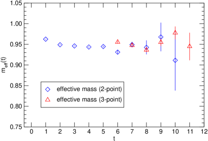
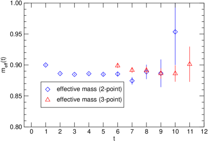
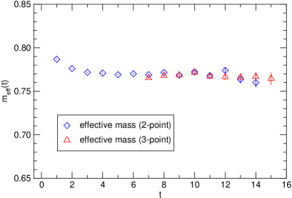
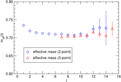
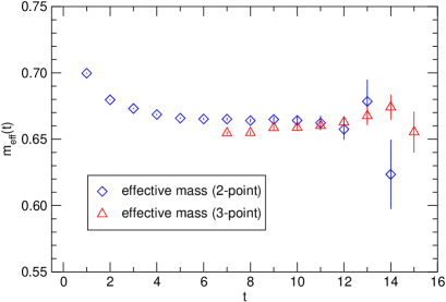
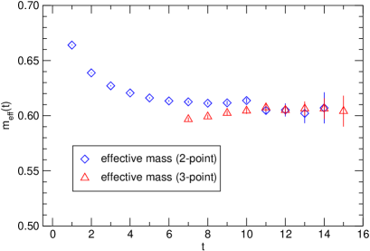
Figures 1 and 2 show the effective mass plots for the 2-point and 3-point functions . We find that the 2-point functions exhibit nice plateaux at for and at for . From this result we take for and for as a reasonable choice for the time separation between the current and the meson source. We also find that the effective masses of the 3-point functions give consistent values with those of the 2-point functions. We fit the 2-point and 3-point functions to exponential functions with single exponent as
| (24) |
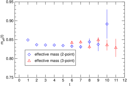
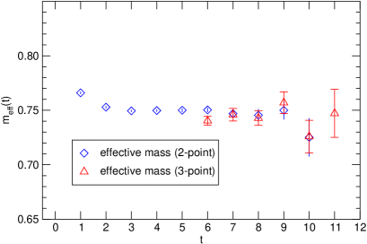
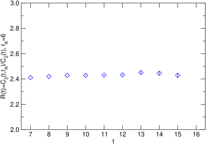
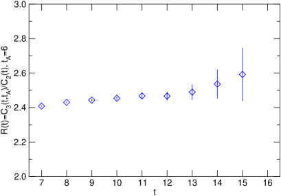
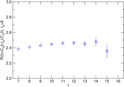
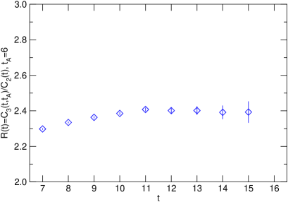
where and are constant parameters and corresponds to the energy of the heavy-light meson. The fit ranges are chosen appropriately by observing the effective mass plots as listed in Table 2. The bare coupling can be obtained by the ratio of the fit parameters as . Alternatively, the coupling is also extracted from the ratio of the 3-point and 2-point functions, , as shown in Figures 3. We find that the fit of the ratio to a constant value gives consistent value with the value of . Since the statistical accuracy is better, we employ to determine in the following analyses. The results are summarized in Table 2.
| 1.80 | 0.1409 | (5,10) | (8,10) | 0.9412(19) | 2.252(21) | 0.612(5) |
| 0.1430 | (5,10) | (8,10) | 0.8839(21) | 2.294(23) | 0.598(5) | |
| 0.1445 | (5,10) | (8,10) | 0.8343(16) | 2.342(13) | 0.591(4) | |
| 0.1464 | (5,10) | (8,10) | 0.7488(17) | 2.381(27) | 0.578(5) | |
| 1.95 | 0.1375 | (8,14) | (11,14) | 0.7669(27) | 2.435( 8) | 0.618(8) |
| 0.1390 | (8,14) | (11,14) | 0.7093(18) | 2.471(16) | 0.615(5) | |
| 0.1400 | (8,14) | (11,14) | 0.6638(15) | 2.461(14) | 0.599(4) | |
| 0.1410 | (8,14) | (11,14) | 0.6098(14) | 2.400(13) | 0.571(4) |
3.3 Physical value of the coupling and chiral extrapolation
The physical value of the coupling is obtained by multiplying the bare value by the renormalization constant. We use the one-loop result of the renormalization factor for the axial vector current
| (25) | |||
where the gauge coupling , 2.816 and , 0.939 for and 1.95, respectively, as given in Ref. [13]. We arrive at the results of for our values in Table 2.
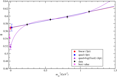
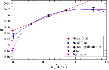
We take the chiral extrapolation of the coupling employing the following fit functions:
corresponding respectively to (a) the linear extrapolation, (b) the quadratic extrapolation, and (c) the quadratic plus chiral log extrapolation where the log coefficient is determined from ChPT [14, 15, 16]. We use three lightest data points for the fit (a), while all the four points for (b) and (c). We obtain physical values of the coupling in the chiral limit as , 0.57(2), 0.52(1) at and , 0.529(10), 0.480(8) at from the fit (a), (b), (c), respectively. Figure 4 shows these chiral extrapolations. We take the average of the results from the linear fit and the quadratic plus chiral log fit as our best value and take half the difference as the systematic error from the chiral extrapolation:
| (26) | |||||
| (27) |
Since we have only two lattice spacings, naive continuum extrapolation would not give a reliable result. However, the results at these two lattice spacings are consistent within quoted errors.111 We do not observe a large scaling violation for as opposed to the case of by CP-PACS collaboration. A possible explanation is that the large scaling violation for might come from the perturbative error of , which is the -improvement coefficient of the light-light axial vector current. If this is the case, receives significant systematic error from the -improvement term for the temporal axial vector current due to the chiral enhancement, whereas does not receive such a systematic error since the corresponding term drops out from the matrix element by the sum over the space. Therefore, we take the result at as our best estimate for the physical value of , and estimate the discretization error of by order counting with GeV. Including the perturbative error of also by order counting, our results for is
| (28) |
In our study, each of the chiral extrapolation error, the perturbative error, and the discretization error is about 6% level. The perturbative error can be removed by employing the nonperturbative renormalization such as the RI-MOM scheme, which is successfully applied to the light-light axial vector current. The discretization error could be reduced by computing on finer lattices. For example, an order counting estimate suggests that the discretization error would be reduced to about 2% on the configurations of CP-PACS at . In contrast, it is not straightforward to control the chiral extrapolation error. It is definitely necessary to use recent unquenched configurations with smallest pion mass GeV. More predominant approach is to employ a fermion formulation possessing the chiral symmetry, such as the overlap fermions, which makes the extrapolation theoretically more transparent.
4 Applicability of the low mode averaging
In this section, we examine under what condition the all-to-all propagator technique, in particular the low mode averaging, is efficient to reduce the statistical error. This would give us a guide to extend our computation to unquenched simulations with smaller quark masses and finer lattices. We mainly investigate the case of in the following.
4.1 Observation of the noise to signal ratio
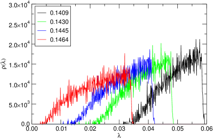
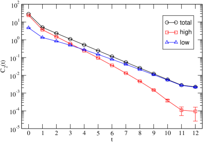
Figure 5 shows the distribution of about 250 lowest eigenmodes for each . Since the contribution of each mode to the correlator is multiplied by , one naively expects that with a fixed number of modes the low mode averaging should be particularly effective for the smallest quark mass. This is indeed true for the 2-point and 3-point heavy-light meson correlators. Figure 6 represents the low and high mode contributions to the 2-point correlators. For the smaller quark mass, the low mode part is indeed more dominant the 2-point correlator in the earlier .

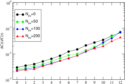
In Figure 7 we show the comparison of the noise to signal ratio of the 2-point functions with different number of low eigenmodes, , 50, 100, 200 for and at . For the smallest quark mass, the statistical error of the 2-point function is 1.5–2 times improved as is changed from 0 to 200. While this is not a drastic improvement, comparing the costs to determine the low-lying eigenmodes and to solve the quark propagator (the latter is 8–10 times larger than the former), there is still an advantage to adopt the low-mode averaging. Projecting out the low-lying modes also improves the cost of solving the quark propagator. These effects are amplified as going to smaller quark mass region.
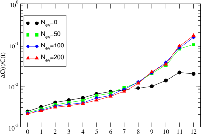
In the region of larger light quark mass, however, the situation is different. The right panel of Fig. 7 shows the noise to signal ratio of the 2-point function for . The noise to signal ratio for achieves about factor 1.3 improvement in the statistical error as we change from 0 to 200. For , on the contrary, the noise to signal ratio with starts to grow more rapidly than that with which keeps to grow steadily. As the result, the low-mode averaging deteriorates the statistical accuracy at this and larger light quark masses.
4.2 High mode and low mode contributions to the noise
To investigate the origin of this behavior, we examine the high mode and low mode contributions to the error of correlator separately.
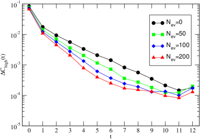
In general, by projecting out larger number of low modes, the high mode part decreases. Therefore one might naively expect that the error also decreases. This is indeed the case for . However for such a naive expectation does not hold. Figs. 8 shows the time dependence of the error for the high mode part of the 2 point correlator with various values of at and . As is displayed in the right panel of Fig. 8, although the error of the high mode contribution to the correlator at does decrease at with larger , the errors of the high mode part at with exceed that with . This clearly indicates that for both the high and low mode parts of the correlator individually have large errors, but when they are combined the error of the total correlator becomes small. In this situation if the low mode part is improved by the low mode averaging, which reduces the error by certain factor, the error of the high mode part of the same size remains unreduced and dominates the error of the correlator.
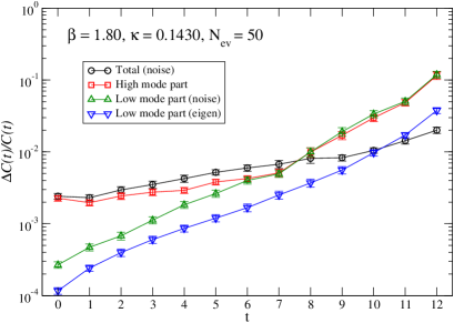
To see it more clearly, let us decompose the 2-point correlator computed by the noisy estimator (corresponding to =0) into the high and low mode parts. The total correlators are computed only with the noisy estimator (denoted as ‘total(noise)’). The high and low mode parts (‘high(noise)’ and ’low(noise)’) are separately computed using the exactly same random source as for the total correlators but projected into the high and low mode spaces with the projection operators and , respectively. Figure 9 displays the statistical errors from the low and high mode parts normalized with the total correlator, in the case of at . For comparison we also show the error of the low mode part determined with low mode averaging (‘low(eigen)’). This figure confirms that the fluctuations of the low and high mode parts are almost the same size and compensate in the total correlator so as to give much smaller error. The errors of the low mode parts, and , exponentially grow with similar rates, while different from that of the total correlator.
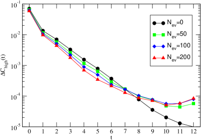
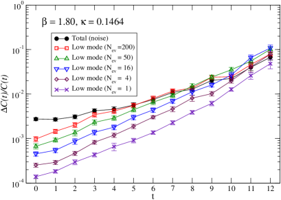
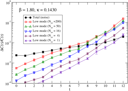
Such a behavior continues as we decrease even down to a few . The right panel of Fig. 10 shows the case of , 4, 16, 50, 200 for , where the fluctuations of the low mode part, , grows similar rates, while absolute values are shifted downward. The left panel of Fig. 10 shows the case for . We observe that the low mode part (‘low(noise)’) does not exceed the signal by large amount, which explains the behavior observed in Fig. 7.
The reason why projecting into the low or high mode part provides a drastic enhancement of the error is still unknown. Although the phenomena themselves are quite interesting and deserves for further studies, in this paper we restrict ourselves within their implication to applicability of the all-to-all propagator technique to the static heavy-light system.
4.3 When is the low mode averaging efficient?
We have seen that the low mode averaging is efficient only if the error of the noisy estimator (not the correlator itself) is dominated by the low mode part. Once the errors from the high and low mode parts of the correlator start to exceed the error of the total correlator, the low mode averaging is no longer effective but it makes the situation even much worse. Our result implies that at and , the rapid growth of the error at in Fig. 7 signals the breakdown of the above condition. For , the noisy estimator without the low mode averaging works better. Thus the low mode averaging is only efficient in the small quark mass region. However, since we have already taken the data and they provided satisfactory statistical accuracy of 2% level, we adopted the result with the low mode averaging propagator at . As for , the low mode averaging has not provided sufficient statistical accuracy for . Thus we adopted the noisy estimator without the low mode averaging at this as was already noted in the previous section.
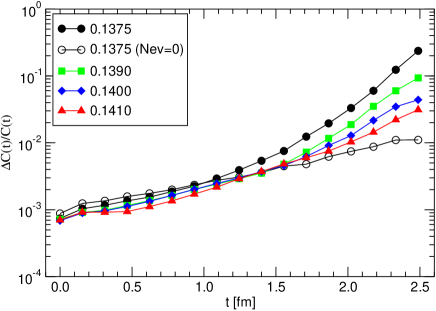
The results at are displayed in Figure 11. The figure shows the noise to signal ratio of the 2-point correlators at each against in physical units. For both the results with and 200 are shown, and the former indeed exhibits smaller statistical error. For all the values of with , the slopes of the exponential growth rate of the noise to signal ratio change around , and beyond that the slopes become steeper as the quark mass increases. This behavior is clearly explained with the breakdown mechanism of the low mode averaging mentioned above.
We can also extract a hint on the lattice spacing dependence of the statistical accuracy by comparing and . Comparison of Figs. 7 and 11 implies that the noise to signal ratio is similar or even smaller for finer lattices. This is partly explained by the fact that as going the finer lattices one has the larger number of lattice points (if the volume is kept unchanged) which are used for the all-to-all propagator. As observed in Figs. 1 and 7, the statistical errors at rapidly increases beyond , which corresponds to fm in physical units. Thus the low mode averaging breaks down almost at the same physical distances at these two lattice spacings. This implies that also on finer lattices of fm, one can extract precise values of coupling from the region fm by applying the same methods as this work, while careful tuning of the smearing function would be indispensable.
5 Conclusion
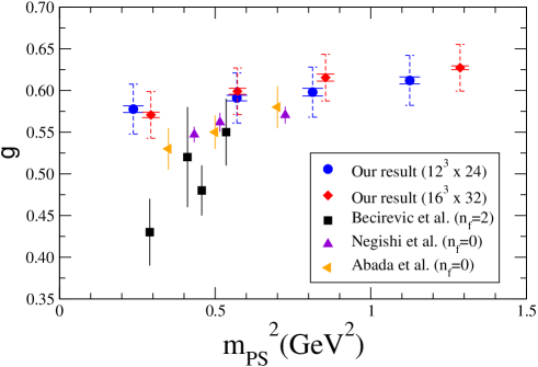
In this paper, we computed the coupling on unquenched lattices using the HYP smearing and the all-to-all propagators. Using the low mode averaging with 200 eigenmodes, the statistical errors are kept sufficiently small for smaller quark masses. On the other hand, as was investigated in Sec. 4 in detail, the low mode averaging is not efficient for larger light quark mass region, where the simple noisy estimator provides better precision. In either case, the statistical error is controlled below 2% level in the chiral limit. We obtained consistent results at two lattice spacings. Our best estimate of the coupling in the static limit is represented in Eq. (28). Figure 12 compares our results with other recent works on the coupling [2, 4, 12]. The improvement in statistical precision is drastic, which proves the power of the improvement techniques employed in this paper.
For future prospects, better control over the systematic error from the chiral extrapolation is indispensable. For this purpose, the configurations with dynamical overlap fermions by JLQCD collaboration would be a good choice [18, 19, 20]. In order to obtain at the physical bottom quark mass, one needs to understand the mass dependence of . Simulations with the charm quark mass region and interpolation with the static limit are desired. The methods adopted in this work are in principle also applicable to other weak matrix elements of the mesons, such as , , and the form factors, and expected to provide high precision results required in precision flavor physics.
Acknowledgments
We would like to thank S. Aoki, M. Della Morte, N. Ishizuka, C. Sachrajda, T. Umeda for fruitful discussions. We are also grateful to S. Fajfer and J. Kamenik for useful comments. We acknowledge JLDG for providing with unquenched configurations from CP-PACS collaboration. The numerical calculations were carried out on the vector supercomputer NEC SX-8 at Yukawa Institute for Theoretical Physics, Kyoto University ,Research Center for Nuclear Physics, Osaka University and also Blue Gene/L at High Energy Accelerator Organization (KEK). The simulation also owes to a gigabit network SINET3 supported by National Institute of Informatics, for efficient data transfer supported by JLDG. This work is supported in part by the Grant-in-Aid of the Ministry of Education (Nos. 19540286, 19740160).
References
- [1] C. G. Boyd and B. Grinstein, Nucl. Phys. B 442, 205 (1995) [arXiv:hep-ph/9402340].
- [2] G. M. de Divitiis, L. Del Debbio, M. Di Pierro, J. M. Flynn, C. Michael and J. Peisa [UKQCD Collaboration], JHEP 9810, 010 (1998) [arXiv:hep-lat/9807032].
- [3] A. Abada, D. Becirevic, Ph. Boucaud, G. Herdoiza, J. P. Leroy, A. Le Yaouanc and O. Pene, JHEP 0402, 016 (2004) [arXiv:hep-lat/0310050].
- [4] D. Becirevic, B. Blossier, Ph. Boucaud, J. P. Leroy, A. LeYaouanc and O. Pene, PoS LAT2005, 212 (2006) [arXiv:hep-lat/0510017].
- [5] W. Detmold, K. Orginos and M. J. Savage, Phys. Rev. D 76, 114503 (2007) [arXiv:hep-lat/0703009].
- [6] M. Della Morte, S. Durr, J. Heitger, H. Molke, J. Rolf, A. Shindler, and R. Sommer [ALPHA Collaboration], Phys. Lett. B 581, 93 (2004) [Erratum-ibid. B 612, 313 (2005)] [arXiv:hep-lat/0307021].
- [7] M. Della Morte, A. Shindler and R. Sommer, JHEP 0508, 051 (2005) [arXiv:hep-lat/0506008].
- [8] A. Hasenfratz and F. Knechtli, Phys. Rev. D 64, 034504 (2001) [arXiv:hep-lat/0103029].
- [9] J. Foley, K. Jimmy Juge, A. O’Cais, M. Peardon, S. M. Ryan and J. I. Skullerud, Comput. Phys. Commun. 172, 145 (2005) [arXiv:hep-lat/0505023].
- [10] T. A. DeGrand and U. M. Heller [MILC collaboration], Phys. Rev. D 65, 114501 (2002) [arXiv:hep-lat/0202001].
- [11] L. Giusti, P. Hernandez, M. Laine, P. Weisz and H. Wittig, JHEP 0404, 013 (2004) [arXiv:hep-lat/0402002].
- [12] S. Negishi, H. Matsufuru and T. Onogi, Prog. Theor. Phys. 117, 275 (2007) [arXiv:hep-lat/0612029].
- [13] A. Ali Khan et al. [CP-PACS Collaboration], Phys. Rev. D 65, 054505 (2002) [Erratum-ibid. D 67, 059901 (2003)] [arXiv:hep-lat/0105015].
- [14] H. Y. L. Cheng, C. Y. L. Cheung, G. L. L. Lin, Y. C. Lin, T. M. Yan and H. L. Yu, Phys. Rev. D 49, 5857 (1994) [Erratum-ibid. D 55, 5851 (1997)] [arXiv:hep-ph/9312304].
- [15] J. F. Kamenik, arXiv:0709.3494 [hep-ph].
- [16] S. Fajfer and J. Kamenik, Phys. Rev. D 74, 074023 (2006) [arXiv:hep-ph/0606278].
- [17] G. P. Lepage, Nucl. Phys. Proc. Suppl. 26, 45 (1992).
- [18] For an overview, H. Matsufuru [JLQCD Collaboration], arXiv:0710.4225 [hep-lat].
- [19] S. Hashimoto et al. [JLQCD collaboration], arXiv:0710.2730 [hep-lat].
- [20] T. Kaneko et al. [JLQCD Collaboration], PoS LAT2006, 054 (2006) [arXiv:hep-lat/0610036].