Fast Computation of Partial Fourier Transforms

Abstract

We introduce two efficient algorithms for computing the partial Fourier transforms in one and two dimensions. Our study is motivated by the wave extrapolation procedure in reflection seismology. In both algorithms, the main idea is to decompose the summation domain of into simpler components in a multiscale way. Existing fast algorithms are then applied to each component to obtain optimal complexity. The algorithm in 1D is exact and takes $O(N\log^{2}N)$ steps. Our solution in 2D is an approximate but accurate algorithm that takes $O(N^{2}\log^{2}N)$ steps. In both cases, the complexities are almost linear in terms of the degree of freedom. We provide numerical results on several test examples.

Keywords. Fast Fourier transform; Multiscale decomposition; Butterfly algorithm; Fractional Fourier transform; Wave extrapolation.

AMS subject classifications. 65R10, 65T50.

1 Introduction

In this paper, we introduce efficient algorithms for the following partial Fourier transform problem in one and two dimensions. In 1D, let $N$ be a large integer and $c^{0}(t)$ be a smooth function on $[0,1]$ with $0\leq c^{0}(t)\leq 1$. We define a sequence of integers $\{c_{x},0\leq x<N\}$ by $c_{x}=N\lceil c^{0}(x/N)\rceil$. Given a sequence of $N$ numbers $\{f_{k},0\leq k<N\}$, the problem is to compute $\{u_{x},0\leq x<N\}$ where

$$u_{x}=\sum_{k<c_{x}}e^{2\pi\imath xk/N}f_{k},$$ (1)

where we use $\imath$ for $\sqrt{-1}$ throughout this paper. In 2D, the problem is defined in a similar way. Now let $c^{0}(t)$ be a smooth function on $[0,1]^{2}$ with $0\leq c^{0}(t)\leq 1$. The array $\{c_{x},0\leq x_{1},x_{2}<N\}$ where $x=(x_{1},x_{2})$ is defined by $c_{x}=N\lceil c^{0}(x/N)\rceil$. Given an array of $N^{2}$ numbers $\{f_{k},0\leq k_{1},k_{2}<N\}$ where $k=(k_{1},k_{2})$, we want to compute $\{u_{x},0\leq x_{1},x_{2}<N\}$ defined by

$$u_{x}=\sum_{|k|<c_{x}}e^{2\pi\imath x\cdot k/N}f_{k}.$$ (2)

Due to the existence of the summation constraints on $k$ in (1) and (2), the fast Fourier transform cannot be used directly here. Direct computation of (1) and (2) has quadratic complexity; i.e., $O(N^{2})$ operations for (1) and $O(N^{4})$ for (2). This can be expensive for large values of $N$, especially in 2D. In this paper, we propose efficient solutions which have almost linear complexity. Our algorithm for the 1D case is exact and takes $O(N\log^{2}N)$ steps, while our solution to the 2D problem is an accurate approximate algorithm with an $O(N^{2}\log^{2}N)$ complexity. We define the summation domain $D$ to be the set of all pairs $(x,k)$ appeared in the summation, namely $D=\{(x,k),k<c_{x}\}$ in 1D and $D=\{(x,k),|k|<c_{x}\}$ in 2D. The main idea behind both algorithms is to partition the summation domain into simple components in a multiscale fashion. Fast algorithms are then invoked on each simple component to achieve maximum efficiency.

The partial Fourier transform appears naturally in several settings. The one which motivates our research is the one-way wave extrapolation method in seismology [4], where one often needs to compute an approximation to the following integral [8]:

$$u_{z}(x)=\int e^{2\pi\imath(x\cdot k+\sqrt{\omega^{2}/v^{2}(x)-k^{2}}\cdot z)}\widehat{u_{0}}(k)dk,$$ (3)

where $\omega$ and $z$ are fixed constants (frequency and extrapolation depth), $v(x)$ is a given function (layer velocity), and $\widehat{u_{0}}(k)$ is the Fourier transform of a function $u_{0}(x)$. The wave modes that correspond to $|k|\leq\omega/v(x)$ are propagating waves, while the ones that correspond to $|k|\geq w/\rho(x)$ are called evanescent. For the purposes of seismic imaging, one is often interested in only the propagating mode and, therefore, we have the following restricted integral to evaluate:

$$\int_{|k|\leq\omega/v(x)}e^{2\pi\imath(x\cdot k+\sqrt{\omega^{2}/v^{2}(x)-k^{2}}\cdot z)}\widehat{u_{0}}(k)dk.$$

To make the computation efficient, the term with the square root under is often approximated with a functional form

$$e^{2\pi\imath\sqrt{\omega^{2}/v^{2}(x)-k^{2}}\cdot z}\approx\sum_{n}f_{n}(x)\,\psi_{n}(k)$$ (4)

with a limited number of terms. The integral then reduces to

$$\sum_{n}f_{n}(x)\,\left[\int_{|k|\leq\omega/v(x)}e^{2\pi\imath x}\widehat{w_{n}}(k)dk.\right]$$

where $\widehat{w_{n}}(k)=\psi_{n}(k)\,\widehat{u_{0}}(k)$. The kernel of this approximation involves computing

$$\int_{|k|\leq w/\rho(x)}e^{2\pi\imath x\cdot k}\widehat{w_{n}}(k)dk,$$

which takes the forms of (1) and (2) after discretization.

The rest of this paper is organized as follows. In Section 2, we describe our 1D algorithm. The 2D algorithm is presented in Section 3. Finally, we conclude with some discussions for future work in Section 4. Throughout this paper, we assume for simplicity that $N$ is an integer power of $2$.

2 Partial Fourier Transform in 1D

2.1 Algorithm description

We define the summation domain by $D=\{(x,k),k<c_{x}\}$. The idea behind our algorithm for computing

$$u_{x}=\sum_{k<c_{x}}e^{2\pi\imath xk/N}f_{k},\quad 0\leq x<N$$

is to decompose $D$ in a multiscale fashion. Starting from the top level box $[0,N]^{2}$, we partition the domain recursively. If a box $B$ is fully inside $D$, it is not subdivided and we keep it inside the decomposition. If a box $B$ is fully outside $D$, it is discarded. Finally, if a box $B$ has parts that belong to both $D$ and $[0,N]^{2}\setminus D$, it is further subdivided into four child boxes with equal size. At the end of this process, our decomposition contains a group of boxes with dyadic sizes and the union of these boxes is exactly equal to $D$ (see Figure 1).

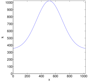
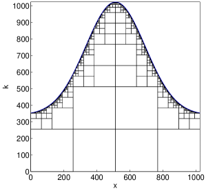
Figure 1: Left: the curve stands for $\{c_{x}\}$ and the summation domain $D$ is the region below the curve. Right: the multiscale decomposition constructed for $D$. The boxes increase their size geometrically as they move away from the curve.

Let us consider a single box $B$ of the decomposition. Suppose that $B$ is of size $s$ and that its lower-left corner of $B$ is $(x^{B},k^{B})$. The part of the summation that associated with $B$ is

$$\sum_{k^{B}\leq k<k^{B}+s}e^{2\pi\imath xk/N}f_{k}$$ (5)

for each $x^{B}\leq x<x^{B}+s$. Denoting $x=x^{B}+x^{\prime}$ and $k=k^{B}+k^{\prime}$, we can write this into a matrix form $Mf$ with

$$(M)_{x^{\prime}k^{\prime}}=e^{2\pi\imath(x^{B}+x^{\prime})(k^{B}+k^{\prime})/N}=e^{2\pi\imath(x^{B}+x^{\prime})k^{B}/N}\cdot e^{2\pi\imath x^{\prime}k^{\prime}/N}\cdot e^{2\pi\imath x^{B}(k^{B}+k^{\prime})/N}.$$

Noticing that the first and the third terms depend only on $x^{\prime}$ and $k^{\prime}$, respectively, we can factorize $M$ as $M=M_{1}\cdot M_{2}\cdot M_{3}$, where $M_{1}$ and $M_{3}$ are diagonal matrices and $M_{2}$ is given by

$$(M_{2})_{x^{\prime}k^{\prime}}=e^{2\pi\imath x^{\prime}k^{\prime}/N}$$ (6)

for $0\leq x^{\prime},k^{\prime}<s$. In fact, (6) is the matrix of the fractional Fourier transform [3], which can be evaluated in only $O(s\log s)$ operations. Furthermore, since both $M_{1}$ and $M_{3}$ are diagonal matrices, (5) can be computed in $O(s\log s)$ steps as well.

Based on this observation, our algorithm takes the following form:

1. Construct a decomposition for $D=\{(x,k),k<c_{x}\}$. Starting from $[0,N]^{2}$, we partition the boxes recursively. A box fully inside the $D$ is not further subdivided. The union of the boxes in the final decomposition is equal to $D$.

2. For $s=1,2,4,8,\cdots,N$, visit all of the boxes of size $s$ in the decomposition. Suppose $B$ is one such box. Compute the summation associated with $B$

   $$\sum_{k^{B}\leq k<k^{B}+s}e^{2\pi\imath xk/N}f_{k}$$

   for $x^{B}\leq x<x^{B}+s$ using the fractional Fourier transform, and add the result to $\{u_{x},x^{B}\leq x<x^{B}+s\}$.

The first step of our algorithm clearly takes at most $O(N\log N)$ steps. To estimate the complexity for the second step, one needs to have a bound on the number of boxes of size $s$. Based on the construction of the decomposition, we know that the center of a box $B$ of size $s$ is at most of distance $s$ away from the curve $\{(x,c_{x})\}$ because otherwise $B$ would have been partitioned further. As a result, the centers of all of the boxes of size $s$ must fall within a band along $\{(x,c_{x})\}$ of width $2s$. Noticing that $c^{0}(t)$ is smooth, the length of $\{(x,c_{x})\}$ is at most $N$. Therefore, the area of the band is at most $O(Ns)$ and there are at most $O(Ns/s^{2})=O(N/s)$ boxes of size $s$. Since we spend $O(s\log s)$ operations in the fractional Fourier transform for each box of size $s$, the number of steps for a fixed $s$ is $O(N/s\cdot s\log s)=O(N\log s)=O(N\log N)$. Finally, summing over all $\log N$ possible values of $s$, we conclude that our algorithm is $O(N\log^{2}N)$. As no approximation has been made, our algorithm is exact.

$N$	$T_{a}$(sec)	$R_{d/a}$	$R_{a/f}$
1024	5.00e-03	3.00e+01	8.57e+00
2048	1.00e-02	6.40e+01	9.27e+00
4096	2.25e-02	1.14e+02	1.09e+01
8192	5.50e-02	1.86e+02	1.36e+01
16384	1.20e-01	3.41e+02	9.23e+00
32768	2.30e-01	7.12e+02	4.15e+01
65536	4.60e-01	1.42e+03	3.98e+01
131072	9.20e-01	2.49e+03	3.68e+01
262144	1.89e+00	4.16e+03	3.48e+01
524288	3.84e+00	8.19e+03	8.30e+01
1048576	8.16e+00	1.29e+04	7.25e+01

Table 1: Top-left: the curve $c_{x}$ and the decomposition of $D$. Top-right: running time of our algorithm as a function of $N$. Bottom: the results for different values of $N$. $T_{a}$: the running time of our algorithm. $R_{d/a}$: the ratio between direct evaluation and our algorithm. $R_{a/f}$: the ratio between our algorithm and one execution of FFT of size $N$.

$N$	$T_{a}$(sec)	$R_{d/a}$	$R_{a/f}$
1024	6.25e-03	2.40e+01	1.07e+01
2048	1.38e-02	4.36e+01	1.27e+01
4096	3.25e-02	7.88e+01	1.54e+01
8192	7.50e-02	1.37e+02	1.86e+01
16384	1.70e-01	2.41e+02	1.09e+02
32768	3.10e-01	5.29e+02	9.92e+01
65536	6.90e-01	8.90e+02	5.89e+01
131072	1.42e+00	1.85e+03	5.83e+01
262144	3.03e+00	2.81e+03	5.64e+01
524288	6.42e+00	4.90e+03	1.17e+02
1048576	1.35e+01	7.77e+03	1.28e+02

Table 2: Top-left: the curve $c_{x}$ and the decomposition of $D$. Top-right: running time of our algorithm as a function of $N$. Bottom: the results for different values of $N$.

$N$	$T_{a}$(sec)	$R_{d/a}$	$R_{a/f}$
1024	3.13e-03	4.48e+01	5.45e+01
2048	6.25e-03	9.60e+01	6.56e+01
4096	1.25e-02	1.92e+02	5.95e+00
8192	4.00e-02	2.56e+02	5.00e+01
16384	9.00e-02	4.27e+02	5.43e+00
32768	1.70e-01	9.04e+02	9.85e+00
65536	3.60e-01	1.82e+03	3.09e+01
131072	7.10e-01	3.46e+03	2.91e+01
262144	1.56e+00	5.46e+03	2.90e+01
524288	3.28e+00	1.04e+04	6.64e+01
1048576	6.66e+00	1.57e+04	6.50e+01

Table 3: Top-left: the curve $c_{x}$ and the decomposition of $D$. Top-right: running time of our algorithm as a function of $N$. Bottom: the results for different values of $N$.

2.2 Numerical results

We apply our algorithm to several test examples to illustrate its properties. All of the results presented here are obtained on a desktop computer with a 2.8GHz CPU. For each example, we use the following notations. $T_{a}$ is the running time of our algorithm in seconds, $R_{d/a}$ is the ratio of the running time of direct evaluation to $T_{a}$, and $R_{a/f}$ is the ratio of $T_{a}$ over the running time of a Fourier transform (timed using FFTW [7]). As our algorithm is $O(N\log^{2}N)$, we expect $R_{d/a}$ to grow almost linearly and $R_{a/f}$ like $\log N$.

Tables 1, 2 and 3 summarize the results for three testing cases. The function in Table 3 corresponds to a 100 Hertz wave propagation through a slice of the Marmousi velocity model [11] taken at 2 km depth. From these examples, we observe clearly that $R_{d/a}$, the ratio between the running times of direct evaluation and our algorithm, indeed grows almost linearly in terms of $N$. Although the ratio $R_{a/f}$ has some fluctuations, its value grows very slowly with respect to $N$.

3 Partial Fourier Transform in 2D

A direct extension of the 1D algorithm to the 2D case would partition the four dimensional summation domain $D=\{(x,k),|k|<c_{x}\}$ with a similar 4D tree structure. However, this does not result in an algorithm with optimal complexity. To see this, let us count the number of boxes of size $s$ in our tree structure. Repeating the argument used in the complexity analysis of the 1D algorithm, we conclude that there are about $N^{3}s/s^{4}=N^{3}/s^{3}$ boxes of size $s$. Even though the computation associated with each box can be done in about $s^{2}\log s$ steps, the total operation count for a fixed $s$ is about $N^{3}/s^{3}\cdot s^{2}\log s=N^{3}/s\log s$, which is much larger than the degree of freedom $N^{2}$ for small values of $s$.

3.1 Algorithm description

Noticing that only $|k|$ appears in the constraint of the 2D partial Fourier transform

$$u_{x}=\sum_{|k|<c_{x}}e^{2\pi\imath x\cdot k/N}f_{k}\quad 0\leq x_{1},x_{2}<N,$$

we study a different set $R=\{(x,r),r<c_{x}\}$ instead.

The algorithm first generates a decomposition for $R$. Similar to the 1D case, we partition the box $[0,N]^{3}$ through recursive subdivision. A box is not further subdivided if it fully resides in $R$. The union of all the boxes inside the decomposition is exactly the set $R$ (see Figure 2).

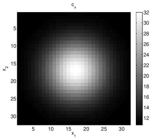
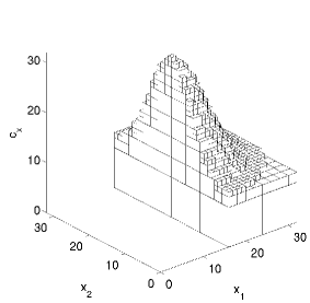
Figure 2: Left: $c_{x}$ is a Gaussian function. Right: a cross section view of the multiscale decomposition of $R$ (the domain below the surface $c_{x}$. Here $N=32$.

The projection of any box of our decomposition onto the $r$ coordinate is a dyadic interval. Let us consider one such interval $A$ of size $s$ and denote $G^{A}$ to be the set of all cubes that project onto $A$. We define $K^{A}$ to be the set $\{k,|k|\in A\}$ and $X^{A}$ to be the image of the points in $G^{A}$ under the projection onto the $(x_{1},x_{2})$ plane. Since $A$ is an interval of size $s$, $K^{A}$ is in fact a band in the $(k_{1},k_{2})$ domain with length $O(N)$ and width $s$. Noticing that the surface $c^{0}(t)$ used to define $\{c_{x},0\leq x_{1},x_{2}<N\}$ is smooth, the set $X_{A}$ is also a band in the $(x_{1},x_{2})$ domain with length $O(N)$ and width $O(s)$ (see Figure 3).

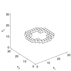
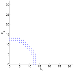
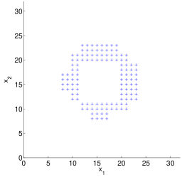
Figure 3: Left: the boxes inside the set $G^{A}$ for an given interval $A$ of the $r$ coordinate. Middle: the set $K^{A}$ in the $(k_{1},k_{2})$ plane. Right: the set $X^{A}$ in the $(x_{1},x_{2})$ plane. The butterfly algorithm in [12] evaluates the summation between $X^{A}$ and $K^{A}$ in almost linear time. Here $N=32$.

The part of the summation associated with the interval $A$ is

$$\sum_{k\in K^{A}}e^{2\pi\imath x\cdot k/N}f_{k}$$ (7)

for $x\in X^{A}$. Since $X^{A}$ and $K^{A}$ are two bands in $[0,N)^{2}$, (7) is indeed a Fourier transform problem with sparse data. To compute (7), we utilize the solution proposed in [12]. This approach is a butterfly algorithm based on [9, 10] and computes an approximation of (7) in $O(\max(|X^{A}|,|K^{A}|)\log(\max(|X^{A}|,|K^{A}|))$ operations, almost linear in terms of the degree of freedom.

Combining these ideas, we have the following algorithm:

1. Construct a decomposition for $R=\{(x,r),r<c_{x}\}$. Starting from $[0,N]^{3}$, we partition the boxes recursively. A box fully inside the $R$ is not further subdivided. The union of the boxes in the final decomposition is equal to $R$.

2. For $s=1,2,4,8,\cdots,N$, visit all the dyadic intervals of size $s$ in the $r$ coordinate. Suppose that $A$ is one such interval. Compute the summation associated with $A$

   $$\sum_{k\in K^{A}}e^{2\pi\imath x\cdot k/N}f_{k}$$

   for $x\in X^{A}$ using the butterfly procedure in [12], and add the result to $\{u_{x},x\in X^{A}\}$.

Let us consider now the complexity of this algorithm. The first step of our algorithm takes only $O(N^{2}\log N)$ steps. In order to estimate the number of operations used in the second step, let us consider a fixed $s$. For each interval $A$ of size $s$, the number of steps used in $O(\max(|X^{A}|,|K^{A}|)\log(\max(|X^{A}|,|K^{A}|))=O(|X^{A}|\log|X^{A}|)+O(|K^{A}|\log|K^{A}|)$. Summing over all boxes of size $s$, we get

$$O\left(\sum_{A:|A|=s}|X^{A}|\log|X^{A}|\right)+O\left(\sum_{A:|A|=s}|K^{A}|\log|K^{A}|\right).$$

Noticing $\sum_{A:|A|=s}|X^{A}|=\sum_{A:|A|=s}|K^{A}|=N^{2}$, the above quantity is clearly bounded by $O(N^{2}\log N)$. Finally, after summing over all different values of $s$, we have a total complexity of order $O(N^{2}\log^{2}N)$.

3.2 Numerical results

We apply our algorithm to several examples in this section. In [12], equivalent charges located at Cartesian grids are used as the low rank representations in the butterfly algorithm to control the accuracy of the method. The size of the Cartesian grid $p$ controls the accuracy of our algorithm. Here, we pick $p$ to be 5 or 9. To quantify the error, we select a set $S\subset\{0,1,\cdots,N-1\}^{2}$ of size 100 and estimate the error by

$$\sqrt{\frac{\sum_{x\in S}|u_{x}-u_{x}^{a}|^{2}}{\sum_{x\in S}|u_{x}|^{2}}}$$

where $\{u_{x}\}$ are the exact results and $\{u_{x}^{a}\}$ are our approximations.

$(N,p)$	$T_{a}$(sec)	$R_{d/a}$	$R_{a/f}$	$E_{a}$
(128,5)	8.50e-01	4.82e+01	9.89e+02	5.25e-04
(256,5)	5.21e+00	1.26e+02	1.59e+03	9.85e-04
(512,5)	3.17e+01	3.76e+02	1.56e+03	7.40e-04
(1024,5)	1.90e+02	1.13e+03	1.61e+03	1.21e-03
(2048,5)	9.60e+02	4.94e+03	1.31e+03	1.20e-03
(128,9)	6.80e-01	6.02e+01	7.25e+02	1.46e-14
(256,9)	5.33e+00	1.29e+02	1.42e+03	8.87e-09
(512,9)	4.18e+01	2.98e+02	1.63e+03	2.17e-08
(1024,9)	2.90e+02	7.49e+02	1.97e+03	9.34e-09
(2048,9)	1.62e+03	2.92e+03	2.10e+03	2.39e-08

Table 4: Top-left: $c_{x}$ when $N=128$. Top-right: running time of our algorithm as a function of $N^{2}$. Bottom: the results for different values of $N$. $T_{a}$: the running time of our algorithm. $R_{d/a}$: the ratio between direct evaluation and our algorithm. $R_{a/f}$: the ratio between our algorithm and one execution of FFT of size $N$. $E_{a}$: the estimated error.

$(N,p)$	$T_{a}$(sec)	$R_{d/a}$	$R_{a/f}$	$E_{a}$
(128,5)	1.31e+00	3.13e+01	1.52e+03	7.11e-04
(256,5)	1.13e+01	6.35e+01	2.91e+03	5.17e-04
(512,5)	7.53e+01	1.65e+02	2.94e+03	1.27e-03
(1024,5)	4.16e+02	5.45e+02	2.62e+03	8.32e-04
(2048,5)	2.10e+03	2.28e+03	2.71e+03	8.88e-04
(128,9)	9.50e-01	4.31e+01	1.01e+03	2.02e-14
(256,9)	1.20e+01	5.75e+01	3.06e+03	6.73e-09
(512,9)	1.08e+02	1.17e+02	4.20e+03	9.35e-09
(1024,9)	6.51e+02	3.46e+02	4.10e+03	1.32e-08
(2048,9)	3.21e+03	1.48e+03	4.12e+03	2.00e-08

Table 5: Top-left: $c_{x}$ when $N=128$. Top-right: running time of our algorithm as a function of $N^{2}$. Bottom: the results for different values of $N$.

$(N,p)$	$T_{a}$(sec)	$R_{d/a}$	$R_{a/f}$	$E_{a}$
(128,5)	6.80e-01	6.02e+01	7.25e+02	4.81e-04
(256,5)	3.35e+00	2.15e+02	8.58e+02	7.17e-04
(512,5)	2.34e+01	5.72e+02	6.18e+02	9.29e-04
(1024,5)	1.14e+02	2.02e+03	6.79e+02	1.04e-03
(2048,5)	5.57e+02	8.83e+03	6.59e+02	1.07e-03
(128,9)	6.00e-01	6.83e+01	6.40e+02	7.66e-15
(256,9)	3.46e+00	1.99e+02	8.52e+02	1.13e-08
(512,9)	2.92e+01	4.09e+02	1.24e+03	1.68e-08
(1024,9)	1.76e+02	1.34e+03	1.14e+03	2.07e-08
(2048,9)	9.39e+02	5.03e+03	1.21e+03	2.62e-08

Table 6: Top-left: $c_{x}$ when $N=128$. Top-right: running time of our algorithm as a function of $N^{2}$. Bottom: the results for different values of $N$.

Similar to the 1D case, the following notations are used: $T_{a}$ is the running time of our algorithm in seconds, $R_{d/a}$ is the ratio of the running time of direct evaluation to $T_{a}$, $R_{a/f}$ is the ratio of $T_{a}$ over the running time of a Fourier transform (timed using FFTW [7]), and finally $E_{a}$ is the estimated error.

The numerical results are summarized in Tables 4, 5 and 6. The function in Table 6 corresponds to a 50 Hertz wave propagation through a slice of the SEG/EAGE velocity model [1] taken at 1.5 km depth. From these numbers, we see that our implementation indeed has a complexity almost linear in terms of the number of grid points. Due to the complex structure of the butterfly procedure, the constant of our algorithm is quite large compared to the one of FFTW.

4 Conclusions and Discussions

In this paper, we introduced two efficient algorithms for computing partial Fourier transforms in one and two dimensions. In both cases, we start by decomposing the appropriate summation domain in a multiscale way into simple pieces and apply existing fast algorithms on each piece to get optimal efficiency. In 1D, the fractional Fourier transform is used. In 2D, we resort to the butterfly algorithm for sparse Fourier transform proposed in [12]. As a result, both of our algorithms are asymptotically only $O(\log N)$ times more expensive than the FFT.

In Tables 4, 5 and 6, we notice that our 2D algorithm has a relatively large constant. One obvious direction of future research is to improve on our current implementation of the butterfly algorithm. Another alternative is to seek different ways for computing the Fourier transforms with sparse data. In the past several years, several algorithms have been developed to address similar oscillatory behavior efficiently (see, for example, [2, 5, 6]). It would be interesting to see whether these ideas can be used in the setting of the Fourier transform with sparse data.

As we mentioned earlier, this research is motivated mostly by the wave extrapolation algorithm in seismic imaging. Our model problem considers only one of the challenges, i.e., the existence of the summation constraint. The other challenge is to improve the evaluation of the $e^{2\pi\imath\sqrt{\omega^{2}/v^{2}(x)-k^{2}}\cdot z}$ term, for example, by approximating it on each of the simple summation components. Research along this direction will be presented in a future report.

Acknowledgments. The first author is partially supported by an Alfred P. Sloan Fellowship and the startup grant from the University of Texas at Austin.

References

- [1] F. Aminzadeh, J. Brac, and T. Kunz. 3-D salt and overthrust models. SEG/EAGE 3-D modeling series. Society of Exploration Geophysicists, 1997.
- [2] A. Averbuch, E. Braverman, R. Coifman, M. Israeli, and A. Sidi. Efficient computation of oscillatory integrals via adaptive multiscale local Fourier bases. Appl. Comput. Harmon. Anal., 9(1):19–53, 2000.
- [3] D. H. Bailey and P. N. Swarztrauber. The fractional Fourier transform and applications. SIAM Rev., 33(3):389–404, 1991.
- [4] B. L. Biondi. 3D Seismic Imaging. Society of Exploration Geophysicists, 2006.
- [5] H. Cheng, W. Y. Crutchfield, Z. Gimbutas, L. F. Greengard, J. F. Ethridge, J. Huang, V. Rokhlin, N. Yarvin, and J. Zhao. A wideband fast multipole method for the Helmholtz equation in three dimensions. J. Comput. Phys., 216(1):300–325, 2006.
- [6] B. Engquist and L. Ying. Fast directional multilevel algorithms for oscillatory kernels. SIAM Journal on Scientific Computing, 29(4):1710–1737, 2007.
- [7] M. Frigo and S. G. Johnson. The design and implementation of FFTW3. Proceedings of the IEEE, 93(2):216–231, 2005. special issue on ”Program Generation, Optimization, and Platform Adaptation”.
- [8] G. F. Margrave and R. J. Ferguson. Wavefield extrapolation by nonstationary phase shift. Geophysics, 64(4):1067–1078, 1999.
- [9] E. Michielssen and A. Boag. A multilevel matrix decomposition algorithm for analyzing scattering from large structures. IEEE Transactions on Antennas and Propagation, 44(8):1086–1093, 1996.
- [10] M. O’Neil and V. Rokhlin. A new class of analysis-based fast transforms. Technical report, Yale University. YALE/DCS/TR1384, 2007.
- [11] R. Versteeg. The Marmousi experience: Velocity model determination on a synthetic complex data set. The Leading Edge, 13:927–936, 1994.
- [12] L. Ying. Sparse Fourier transform via butterfly algorithm. Technical report, University of Texas at Austin, 2008. arXiv:0801.1524v1.