Synchrotron Self-Compton Analysis of TeV X-ray Selected BL Lacertae Objects

Abstract

We introduce a methodology for analysis of multiwavelength data from X-ray selected BL Lac (XBL) objects detected in the TeV regime. By assuming that the radio–through–X-ray flux from XBLs is nonthermal synchrotron radiation emitted by isotropically-distributed electrons in the randomly oriented magnetic field of a relativistic blazar jet, we obtain the electron spectrum. This spectrum is then used to deduce the synchrotron self-Compton (SSC) spectrum as a function of the Doppler factor, magnetic field, and variability timescale. The variability timescale is used to infer the comoving blob radius from light travel-time arguments, leaving only two parameters. With this approach, we accurately simulate the synchrotron and SSC spectra of flaring XBLs in the Thomson through Klein-Nishina regimes. Photoabsorption by interactions with internal jet radiation and the intergalactic background light (IBL) is included. Doppler factors, magnetic fields, and absolute jet powers are obtained by fitting the HESS and Swift data of the recent giant TeV flare observed from PKS 2155–304 (catalog ). For the HESS and Swift data from 28 and 30 July 2006, respectively, Doppler factors $\gtrsim 60$ and absolute jet powers $\gtrsim 10^{46}$ ergs s^-1 are required for a synchrotron/SSC model to give a good fit to the data, for a low intensity of the IBL and a ratio of 10 times more energy in hadrons than nonthermal electrons. Fits are also made to a TeV flare observed in 2001 from Mkn 421 (catalog ) which require Doppler factors $\gtrsim 30$ and jet powers $\gtrsim 10^{45}$ erg s^-1.

1 INTRODUCTION

Radiation from blazars is thought to originate from a relativistic jet, closely aligned with our line of sight, that is powered by a supermassive black hole at the nucleus of an active galaxy. Blazars exhibit strong, rapidly-varying emission throughout the electromagnetic spectrum from radio to $\gamma$-rays. The broadband spectral energy distributions (SEDs) of blazars consist of two components (e.g.  Mukherjee et al., 1997; Weekes, 2003): a low energy component that peaks at infrared or optical energies, and a high energy component that peaks at MeV–GeV $\gamma$-ray energies, and often extends to very high-energy (VHE) $\gamma$-rays. BL Lacertae (BL Lac) objects are a subclass of blazars distinguished by their weakness or absence of broad emission lines in a quasar-like optical spectrum. BL Lac objects are often further sub-divided into those that have low energy components peaking in the optical (known as low frequency peaked or radio selected BL Lacs [RBLs]) and those that have low energy components peaking in the X-rays (high frequency peaked or X-ray selected BL Lacs [XBLs]).

There are two broad classes of models which are used to describe these observations: leptonic models, in which the emission is primarily from relativistic electrons and positrons; and hadronic models, in which the emission is primarily from protons and atomic nuclei. In the leptonic models (see, e.g., Böttcher, 2007, for a review), the low-energy component is interpreted as synchrotron emission from leptons, and the high-energy component as radiation from target photons Compton up-scattered by relativistic jet leptons. The target photons can originate from the synchrotron radiation (synchrotron self-Compton, or SSC; Bloom & Marscher, 1996), as well as external sources, e.g., the broad-line region (Sikora et al., 1994), a dusty torus (Błażejowski et al., 2000), and/or the accretion disk (Dermer et al., 1992; Dermer & Schlickeiser, 1993). In hadronic models (see, e.g., Mannheim & Biermann, 1992; Mücke & Protheroe, 2001; Atoyan & Dermer, 2003), the low-energy component is still interpreted as synchrotron emission from relativistic leptons, but the high energy component originates from proton synchrotron or photopion production initiated by interactions between protons and soft photons. The high-energy synchrotron and Compton emissions create, following cascading and absorption of $\gamma$-rays by the ambient photons, a second hadronicly induced $\gamma$-ray emission component.

Blazar modeling has generally concentrated on leptonic processes to model simultaneous multi-wavelength data (e.g., Ghisellini & Madau, 1996; Li & Kusunose, 2000; Böttcher & Chiang, 2002; Böttcher et al., 2002; Joshi & Böttcher, 2007). In the standard time-dependent leptonic blazar models, the low- and high-energy components in the SEDs are simultaneously fit by injecting nonthermal electrons (including positrons) into the jet and allowing the electrons to evolve through radiative and adiabatic cooling.

In this paper, we use a different approach to model the SEDs of XBLs. In § 2, we fit the optical/X-ray $\nu F_{\nu}$ spectrum, and use this spectral form to deduce the electron distribution in the jet assuming that this emission is nonthermal lepton synchrotron radiation. We then use this electron distribution to calculate the high-energy SSC component. The SSC flux is then precisely given by the inferred electron distribution and a small set of well-constrained observables. The full Compton cross section, accurate for relativistic electrons from the Thomson through the Klein-Nishina regime, is used in the derivation. We take into account $\gamma\gamma$ absorption by high energy interactions with low energy jet radiation and by interactions with the intergalactic background light (IBL). We then apply this formulation to the recently observed giant TeV flare in the XBL PKS 2155–304 (catalog ) (§ 3, Aharonian et al., 2007a; Foschini et al., 2007) as well as to the March 2001 TeV flare observed from Mkn 421 (catalog ) with HEGRA and RXTE (§4, Aharonian et al., 2002; Fossati et al., 2008). Allowed values of mean magnetic field $B$ and Doppler factor $\delta_{\rm D}$ are obtained by fitting the X/$\gamma$-ray spectrum of PKS 2155–304 (catalog ) in § 3 and Mkn 421 (catalog ) in § 4, and used to derive the apparent isotropic jet luminosity. The results are discussed and summarized in § 5.

2 ANALYSIS

Blazars vary on timescales from days to months at radio frequencies (e.g., Böttcher et al., 2003; Villata et al., 2004), and on timescales as short as a few hours or less at X/$\gamma$-ray energies (e.g., Tagliaferri et al., 2003; Foschini et al., 2006). Photoabsorption arguments (Maraschi et al., 1992) and observations of superluminal motions (Vermeulen & Cohen, 1994) show that the emission region is moving with relativistic speeds.

We consider a one-zone spherical blob of relativistic plasma moving with Lorentz factor $\Gamma=(1-\beta^{2})^{-1/2}$. Quantities in the observer’s frame are unprimed, and quantities in the frame comoving with the jet blob are primed, so that the comoving volume of the blob is $V^{\prime}_{b}=4\pi R_{b}^{\prime 3}/3$, where $R_{b}^{\prime}$ is the comoving radius of the emitting blob. The angle that the jet makes with the observer’s line of sight is denoted by $\theta\equiv\arccos\ \mu$, and the Doppler factor is given by $\delta_{\rm D}=[\Gamma(1-\beta\mu)]^{-1}$. Distinct, rapid high-energy flares observed in blazars imply that the emitting region is confined to a small volume with a comoving variability timescale $t_{v}^{\prime}$, limited by light travel time, given by

$$t_{v}^{\prime}\gtrsim\frac{R_{b}^{\prime}}{c}\;.$$ (1)

For the observer, the measured variability timescale is

$$t_{v}\gtrsim t_{v,min}=\frac{(1+z)R_{b}^{\prime}}{\delta_{\rm D}c}.$$ (2)

In the remainder of this section, we compute the SSC spectrum using the electron spectrum derived with the $\delta$-approximation for synchrotron radiation (§ 2.1). We then derive the SSC spectrum using a model-dependent approach to obtain the electron spectrum by integrating over the exact synchrotron emissivity and minimizing $\chi^{2}$ (§ 2.2). We compare the $\delta$-approximation and the full expression for synchrotron in § 2.3 and the Thomson and full Compton expressions in § 2.4. We determine the $\gamma\gamma$ absorption opacity from jet radiation (§ 2.5), and present constraints based on power available in the jet (§ 2.6). The fitting technique using the exact synchrotron expression and the full Compton cross-section is described in § 2.7. Two versions of the Heaviside function are used: $H(x)=0$ for $x<0$ and $H(x)=1$ for $x\geq 0$; as well as $H(x;x_{1},x_{2})=1$ for $x_{1}\leq x\leq x_{2}$ and $H(x;x_{1},x_{2})=0$ everywhere else.

2.1 SSC Emission in the $\delta$-approximation for synchrotron

The $\delta$-approximation for the synchrotron spectrum is useful in that it allows one directly to obtain the electron spectrum and then calculate the predicted $\nu F_{\nu}$ SSC spectrum, $f_{\epsilon}^{SSC}$, in terms of the observed $\nu F_{\nu}$ synchrotron spectrum, $f_{\epsilon}^{syn}$, where $\epsilon=h\nu/m_{e}c^{2}$ is the emitted photon’s dimensionless energy in the observer’s frame. We demonstrate this approach in this section. The $\delta$-approximation is also used to calculate jet power. For detailed spectral modeling, however, a more accurate expression is needed (§ 2.2).

The $\delta$-approximation for the synchrotron flux is

$$f_{\epsilon}^{syn}\cong{\delta_{\rm D}^{4}\over 6\pi d_{L}^{2}}\;c\sigma_{\rm T}U_{B}\gamma^{\prime 3}_{s}N_{e}^{\prime}(\gamma^{\prime}_{s})$$ (3)

(e.g.  Dermer & Schlickeiser, 2002). Here $d_{L}$ is the luminosity distance, $c$ is the speed of light, $\sigma_{\rm T}$ is the Thomson cross section, $N_{e}^{\prime}(\gamma^{\prime}_{s})$ is the comoving electron distribution,

$$\gamma^{\prime}_{s}=\sqrt{{\epsilon(1+z)\over\delta_{\rm D}\epsilon_{B}}}=\sqrt{\epsilon^{\prime}\over\epsilon_{B}}\;,$$ (4)

is a synchrotron-emitting electron’s Lorentz factor, and

$$U_{B}=\frac{B^{2}}{8\pi}$$

is the mean comoving magnetic-field energy density of the randomly-oriented comoving field with mean intensity $B$. In eq. (4), $z$ is the redshift of the object and $\epsilon_{B}=B/B_{cr}$, where $B_{cr}=4.414\times 10^{13}$ G is the critical magnetic field. Note that the magnetic field, $B$, is defined in the comoving frame, despite being unprimed. The $\delta$-approximation is accurate for spectral indices approximately $2.0\leq p\leq 3.5$ (where the electron distribution is $N^{\prime}_{e}(\gamma^{\prime})\propto\gamma^{\prime-p}$).

The comoving electron distribution, $N_{e}^{\prime}(\gamma^{\prime}_{s})$, can be found in terms of $f_{\epsilon}^{syn}$ from eq. (3):

$$N_{e}^{\prime}(\gamma^{\prime}_{s})=V^{\prime}_{b}n^{\prime}_{e}(\gamma^{\prime}_{s})\cong{6\pi d_{L}^{2}f_{\epsilon}^{syn}\over c\sigma_{\rm T}U_{B}\delta_{\rm D}^{4}\gamma^{\prime 3}_{s}}\;.$$ (5)

The synchrotron emissivity, $\dot{n}_{syn}(\epsilon)$ (photons cm^-3 s^-1 $\epsilon^{-1}$), is given by

$$\dot{n}^{\prime}_{syn}(\epsilon^{\prime})\cong{2\over 3}\;{c\sigma_{\rm T}u_{B}}\;\epsilon^{\prime-1/2}\epsilon_{B}^{-3/2}\;n^{\prime}_{e}\left(\gamma^{\prime}_{s}\right)\;,$$ (6)

with $u_{B}=U_{B}/m_{e}c^{2}$. Using this and eq. (5), one can determine the synchrotron photon number density,

$$n^{\prime}_{syn}(\epsilon^{\prime})\cong{R_{b}^{\prime}\over c}\;\dot{n}_{syn}^{\prime}(\epsilon^{\prime})\;\cong{3d_{L}^{2}f_{\epsilon}^{syn}\over m_{e}c^{3}R^{\prime 2}_{b}\delta_{\rm D}^{4}\epsilon_{B}^{2}\gamma^{\prime 4}_{s}}\;.$$ (7)

This can be converted to a radiation energy density through the relation

$$u^{\prime}(\epsilon^{\prime})=\epsilon^{\prime}m_{e}c^{2}n^{\prime}_{syn}(\epsilon^{\prime})=\frac{3d_{L}^{2}f_{\epsilon}^{syn}}{cR_{B}^{\prime 2}\delta_{\rm D}^{4}\epsilon^{\prime}}=\frac{3d_{L}^{2}(1+z)^{2}f_{\epsilon}^{syn}}{c^{3}t^{2}_{v,min}\delta_{\rm D}^{6}\epsilon^{\prime}}\ ,$$ (8)

where we have made use of eqs. (4) and (2).

The SSC emissivity, integrated over volume, for isotropic and homogeneous photon and electron distributions is given by

$$\epsilon^{\prime}_{s}J^{\prime}_{SSC}(\epsilon^{\prime}_{s})={3\over 4}c\sigma_{\rm T}\epsilon^{\prime 2}_{s}\int_{0}^{\infty}d\epsilon^{\prime}\;{u^{\prime}(\epsilon^{\prime})\over\epsilon^{\prime 2}}\int_{\gamma^{\prime}_{min}}^{\gamma^{\prime}_{max}}d\gamma^{\prime}\;{N_{e}^{\prime}(\gamma^{\prime})\over\gamma^{\prime 2}}\;F_{\rm C}(q,\Gamma_{e})\;,$$ (9)

where for a homogeneous distribution, $\epsilon^{\prime}_{s}J^{\prime}_{SSC}(\epsilon^{\prime}_{s})=V^{\prime}_{b}\epsilon^{\prime}_{s}j^{\prime}_{SSC}(\epsilon^{\prime}_{s})$ and $\epsilon^{\prime}_{s}$ is the scattered photon’s dimensionless energy in the blob frame. In eq. (9) the Compton scattering kernel for isotropic photon and electron distributions is

$$F_{\rm C}(q,\Gamma_{e})=\biggr{[}2q\ln q+(1+2q)(1-q)+{1\over 2}{(\Gamma_{e}q)^{2}\over(1+\Gamma_{e}q)}(1-q)\biggr{]}\;H\;\left(q;{1\over 4\gamma^{\prime 2}},1\right)$$ (10)

(Jones, 1968; Blumenthal & Gould, 1970), where

$$q\equiv{\epsilon^{\prime}_{s}/\gamma^{\prime}\over\Gamma_{e}(1-\epsilon^{\prime}_{s}/\gamma^{\prime})}\;\;{\rm and}\;\;\Gamma_{e}=4\epsilon^{\prime}\gamma^{\prime}\;.$$ (11)

The limits on $q$ are

$$\frac{1}{4\gamma^{\prime 2}}\ \leq\ q\ \leq 1\ ,$$ (12)

which imply the limits of the integration over $\gamma^{\prime}$:

$$\gamma^{\prime}_{min}={1\over 2}\epsilon^{\prime}_{s}\;\left(1+\sqrt{1+{1\over\epsilon^{\prime}\epsilon^{\prime}_{s}}}\right)$$ (13)

and

$$\gamma^{\prime}_{max}={\epsilon^{\prime}\epsilon^{\prime}_{s}\over\epsilon^{\prime}-\epsilon^{\prime}_{s}}H(\epsilon^{\prime}-\epsilon^{\prime}_{s})\;+\;\gamma^{\prime}_{2}H(\epsilon^{\prime}_{s}-\epsilon^{\prime})\ .$$ (14)

The upper limit, eq. (14), takes into account Compton up– and down–scattering. In principle, the maximum accelerated electron energy $\gamma^{\prime}_{2}$ can be determined from particle acceleration theory.

The $\nu F_{\nu}$ SSC spectrum is given by

$$f_{\epsilon_{s}}^{SSC}=\frac{\delta_{\rm D}^{4}\epsilon^{\prime}_{s}J^{\prime}_{SSC}(\epsilon^{\prime}_{s})}{4\pi d_{L}^{2}}\ .$$ (15)

Inserting eq. (9) into eq. (15) and using eqs. (8) and (5) gives

$$f_{\epsilon_{s}}^{SSC}=\left({3\over 2}\right)^{3}\;{d_{L}^{2}\epsilon_{s}^{\prime 2}\over R_{b}^{\prime 2}c\delta_{\rm D}^{4}U_{B}}\;\int_{0}^{\infty}d\epsilon^{\prime}\;{f_{\tilde{\epsilon}}^{syn}\over\epsilon^{\prime 3}}\;\int_{\gamma^{\prime}_{min}}^{\gamma^{\prime}_{max}}\;d\gamma^{\prime}\ {F_{\rm C}(q,\Gamma_{e})f_{\hat{\epsilon}}^{syn}\over\gamma^{\prime 5}}\;,$$ (16)

where

$$\tilde{\epsilon}={\delta_{\rm D}\epsilon^{\prime}\over 1+z}\;,$$

$$\hat{\epsilon}={\delta_{\rm D}\epsilon_{B}\gamma^{\prime 2}\over 1+z}\;,\;$$

and

$$\epsilon^{\prime}_{s}={(1+z)\epsilon_{s}\over\delta_{\rm D}}\;.$$

Using eq. (2) to give an estimate of the blob’s radius,

$$R^{\prime}_{b}\cong\frac{c\delta_{\rm D}t_{v,min}}{1+z}\ ,$$

we obtain

$$f_{\epsilon_{s}}^{SSC}={27\pi\epsilon_{s}^{\prime 2}\over c^{3}}\ \left(\frac{d_{L}}{1+z}\right)^{2}\ \left(\frac{1}{t_{v,min}\delta_{\rm D}^{3}B}\right)^{2}\ \int_{0}^{\infty}d\epsilon^{\prime}\;{f_{\tilde{\epsilon}}^{syn}\over\epsilon^{\prime 3}}\;\int_{\gamma^{\prime}_{min}}^{\gamma^{\prime}_{max}}\;d\gamma^{\prime}\;{F_{\rm C}(q,\Gamma_{e})f_{\hat{\epsilon}}^{syn}\over\gamma^{\prime 5}}\;.$$ (17)

The observed SSC spectrum in eq. (17) is a function of three observables, namely redshift $z$, the observed synchrotron spectrum ($f_{\epsilon}^{syn}$), and the variability timescale ($t_{v,min}$), and two unknowns, $\delta_{\rm D}$ and $B$. We use spectral modeling to constrain these two unknowns. Note the quantity $t_{v,min}\delta_{\rm D}^{3}B$ is nearly, but not quite, a constant due to the appearance of $\delta_{\rm D}$ in the integrand and the limits.

2.2 SSC Emission with Exact Synchrotron Expression

Crusius & Schlickeiser (1986) have derived an expression for the synchrotron emissivity from isotropic electrons in a randomly-oriented magnetic field (see also Ghisellini et al., 1988),

$$\epsilon^{\prime}J_{syn}^{\prime}(\epsilon^{\prime})=\frac{\sqrt{3}\epsilon^{\prime}e^{3}B}{h}\int^{\infty}_{1}d\gamma^{\prime}\ N_{e}^{\prime}(\gamma^{\prime})\ R(x)$$ (18)

where $e$ is the fundamental charge, $h$ is Planck’s constant,

$$x=\frac{4\pi\epsilon^{\prime}m_{e}^{2}c^{3}}{3eBh\gamma^{\prime 2}}\ ,$$

$$R(x)=\frac{x}{2}\int_{0}^{\pi}d\theta\ \sin\theta\ \int^{\infty}_{x/\sin\theta}dt\ K_{5/3}(t),$$

and $K_{5/3}(t)$ is the modified Bessel function of the second kind of order 5/3. The function $R(x)$ can be approximated as follows:

$$\log(R)=A_{0}+A_{1}y+A_{2}y^{2}+A_{3}y^{3}+A_{4}y^{4}+A_{5}y^{5}$$ (19)

where $y=\log(x)$ and the values of the coefficients are given in Table 1. These approximations are accurate to $\sim 1$% in the range $10^{-2}<x<10^{1}$; outside this range, the asymptotic expressions from Crusius & Schlickeiser (1986),

$$R(x)=\left\{\begin{array}[]{ll}1.80842\ x^{1/3}&x\ll 1\\ \frac{\pi}{2}e^{-x}\left[1-\frac{99}{162x}\right]&x\gg 1\\ \end{array}\right.\ ,$$ (20)

can be used. They are accurate to better than 5% outside the range $10^{-2}<x<10^{1}$.

The synchrotron flux is then given by

$$f_{\epsilon}^{syn}=\frac{\delta_{\rm D}^{4}\epsilon^{\prime}J_{syn}^{\prime}(\epsilon^{\prime})}{4\pi d_{L}^{2}}=\frac{\sqrt{3}\delta_{\rm D}^{4}\epsilon^{\prime}e^{3}B}{4\pi hd_{L}^{2}}\int^{\infty}_{1}d\gamma^{\prime}\ N_{e}^{\prime}(\gamma^{\prime})\ R(x)\ .$$ (21)

Using this and eqs. (8) and (9) one gets the SSC emissivity,

$$\epsilon_{s}^{\prime}J_{SSC}^{\prime}(\epsilon^{\prime}_{s})=\frac{9\sigma_{\rm T}d_{L}^{2}\epsilon^{\prime 2}_{s}}{4\delta_{\rm D}^{4}R^{\prime 2}_{b}}\int^{\infty}_{0}\ d\epsilon^{\prime}\ \frac{f_{\epsilon}^{syn}}{\epsilon^{\prime 3}}\ \int^{\gamma^{\prime}_{max}}_{\gamma^{\prime}_{min}}d\gamma^{\prime}\ \frac{N^{\prime}_{e}(\gamma^{\prime})}{\gamma^{\prime 2}}F_{C}(q,\Gamma)\ ,$$ (22)

and the observed flux (using eq. [15]),

$$f_{\epsilon_{s}}^{SSC}=\frac{9}{16}\frac{(1+z)^{2}\sigma_{\rm T}\epsilon^{\prime 2}_{s}}{\pi\delta_{\rm D}^{2}c^{2}t_{v,min}^{2}}\int^{\infty}_{0}\ d\epsilon^{\prime}\ \frac{f_{\epsilon}^{syn}}{\epsilon^{\prime 3}}\ \int^{\gamma^{\prime}_{max}}_{\gamma^{\prime}_{min}}\ d\gamma^{\prime}\ \frac{N^{\prime}_{e}(\gamma^{\prime})}{\gamma^{\prime 2}}F_{C}(q,\Gamma)\ .$$ (23)

2.3 Comparison of Exact Synchrotron Expression with $\delta$-approximation

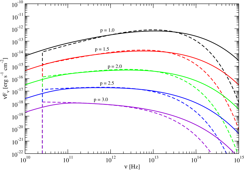
Figure 1: A comparison between the exact synchrotron expression (solid curves) and the $\delta$-approximation (dashed curves) computed for various electron spectral indices.

In Fig. 1 we compare the exact synchrotron expression for synchrotron radiation, eq. (21), with the $\delta$-approximation, eq. (3). In this calculation, we use

$$N_{e}^{\prime}(\gamma^{\prime})=K_{e}\ \gamma^{\prime-p}\ \exp\left(\frac{-\gamma^{\prime}}{\gamma^{\prime}_{c}}\right)\ H(\gamma^{\prime}-\gamma^{\prime}_{1})$$ (24)

for the electron distribution, with $K_{e}=10^{49}$, $\gamma^{\prime}_{1}=10^{2}$, $\gamma^{\prime}_{c}=10^{3}$, $z=0.116$, and various values of $p$. We use $\delta_{\rm D}=100$, $B=10$ mG, and $t_{v,min}=300$ s. This figure shows that the approximation is quite accurate near the center of the spectrum, but loses accuracy at low and high frequencies. At the high frequencies, in particular, the improved accuracy of the full expression is needed to accurately fit the VHE $\gamma$-ray data.

2.4 SSC in the Thomson Regime

Here we compare results using the Thomson cross section with the full Compton cross section derived above. Representing the synchrotron spectrum as a monochromatic radiation field with comoving energy density $u^{\prime}_{syn}$, the SSC flux can be approximated in the Thomson regime, analogous to eq. (3), by the expression

$$f_{\epsilon_{s}}^{SSC,T}\cong{\delta_{\rm D}^{4}\over 6\pi d_{L}^{2}}\;c\sigma_{\rm T}u^{\prime}_{syn}\gamma_{T}^{\prime 3}N_{e}^{\prime}(\gamma^{\prime}_{T})\ ,$$ (25)

where

$$\gamma^{\prime}_{T}=\sqrt{\frac{(1+z)\epsilon_{s}}{\delta_{\rm D}\epsilon^{\prime}}}\ .$$ (26)

Inserting eqs. (8) and (5) into this, one gets

$$label{festhom}f_{\epsilon_{s}}^{SSC,T}\cong\frac{24\pi}{c^{3}}\ \frac{(1+z)^{2}d_{L}^{2}f_{\epsilon}^{syn}(\epsilon_{syn}^{pk})f_{\epsilon}^{syn}(\epsilon_{syn})}{(t_{v,min}B\delta_{\rm D}^{3})^{2}}\ ,$$ (27)

where

$$\epsilon_{syn}=\frac{\epsilon_{s}\epsilon_{B}\delta_{\rm D}}{\epsilon_{syn}^{pk}(1+z)}\ .$$ (28)

Here, if $f_{e_{s}}^{SSC}$ and $f_{\epsilon}^{syn}$ are given from observations, and the redshift (and hence the luminosity distance) of the object is known, then the quantity $t_{v,min}B\delta_{\rm D}^{3}$ is a constant in the Thomson regime. Due to the appearance of $\delta_{\rm D}$ in the integrals of eq. (15) or (23), this dependence does not strictly hold when the full Compton cross section is used, but describes the general behavior. The constraint $t_{v,min}B\delta_{\rm D}^{3}=\textrm{constant}$ was derived previously by Tavecchio et al. (1998).

In order to treat SSC emission in the Thomson regime in the formulation of § 2.1 or § 2.2, one need only replace eq. (10) by

$$F_{T}(q_{T})=\frac{2}{3}\left(1\ -\ q_{T}\right)H\left(q_{T};\frac{1}{4\gamma^{\prime 2}},1\right)\ ,$$ (29)

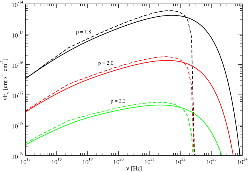
Figure 2: A comparison of SSC calculated with the full Compton cross section (solid curves) and the Thomson cross section (dashed curves) for various electron spectral indices.

where $q_{T}=\epsilon^{\prime}_{s}/(4\gamma^{\prime 2}\epsilon^{\prime})$. A comparison between the Compton and Thomson calculations for a particular model with a power-law electron distribution with an exponential cut off is shown in Fig. 2. As can be seen, the full Klein-Nishina expression gives substantially different results, and would result in significantly different parameter fits. This demonstrates that the full Klein-Nishina expression is necessary to do accurate spectral modeling at $\gamma$-ray energies.

2.5 $\gamma\gamma$ Photoabsorption

2.5.1 Exact Internal Photoabsorption

Here we calculate the $\gamma\gamma$ absorption optical depth, $\tau_{\gamma\gamma}$, due to interactions with the internal synchrotron radiation field. This will, naturally, be a function of the synchrotron spectrum, $f^{syn}_{\epsilon}$. Absorption will modify the high energy SSC spectrum by the factor

$$\frac{1\ -\ e^{-\tau_{\gamma\gamma}}}{\tau_{\gamma\gamma}},$$

and the absorbed $\gamma$-rays will be reinjected to form a second injection component of high-energy leptons. In this paper, we neglect the additional cascade $\gamma$-rays formed by pair reinjection, which is a good assumption when the absorbed energy is a small fraction of the total $\gamma$-ray energy.

The photoabsorption optical depth for a $\gamma$-ray photon with energy $\epsilon_{1}$ in a radiation field with spectral photon density $n(\epsilon^{\prime},\mu^{\prime};r^{\prime})$ is (Gould & Schréder, 1967; Brown et al., 1973)

$$\tau_{\gamma\gamma}(\epsilon^{\prime}_{1})=\int_{r_{1}^{\prime}}^{r_{2}^{\prime}}dr^{\prime}\int_{-1}^{1}d\mu^{\prime}(1-\mu^{\prime})\ \int_{2/\epsilon^{\prime}_{1}(1-\mu^{\prime})}^{\infty}d\epsilon^{\prime}\;\sigma_{\gamma\gamma}[\epsilon^{\prime}\epsilon^{\prime}_{1}(1-\mu^{\prime})]n^{\prime}(\epsilon^{\prime},\mu^{\prime};r^{\prime})\ .$$ (30)

For a uniform isotropic radiation field in the comoving frame, $n_{rad}(\epsilon^{\prime},\mu^{\prime};r^{\prime})\approx n_{rad}(\epsilon^{\prime})/2$, so that

$$\tau_{\gamma\gamma}(\epsilon^{\prime}_{1})\cong R_{b}^{\prime}\int_{0}^{\infty}d\epsilon^{\prime}\;\sigma_{\gamma\gamma}(\epsilon^{\prime},\epsilon^{\prime}_{1})n_{rad}^{\prime}(\epsilon^{\prime})\ .$$ (31)

Inserting the form of the absorption cross-section, one gets

$$\tau_{\gamma\gamma}(\epsilon^{\prime}_{1})=\frac{R_{b}^{\prime}\pi r_{e}^{2}}{\epsilon_{1}^{\prime 2}}\int^{\infty}_{1/\epsilon^{\prime}_{1}}d\epsilon^{\prime}\ n_{rad}^{\prime}(\epsilon^{\prime})\ \bar{\phi}(s_{0})\$$ (32)

where $s_{0}=\epsilon^{\prime}\epsilon^{\prime}_{1}$,

$$\bar{\phi}(s_{0})=\frac{1+\beta_{0}^{2}}{1-\beta_{0}^{2}}\ln w_{0}-\beta_{0}^{2}\ln w_{0}-\frac{4\beta_{0}}{1-\beta_{0}^{2}}$$ (33)

$$+2\beta_{0}+4\ln w_{0}\ln(1+w_{0})-4L(w_{0})\ ,$$

$\beta_{0}^{2}=1-1/s_{0}$, $w_{0}=(1+\beta_{0})/(1-\beta_{0})$, and

$$L(w_{0})=\int^{w_{0}}_{1}dw\ w^{-1}\ln(1+w)\ .$$ (34)

Substituting the internal synchrotron radiation field, eq. (7), for $n_{rad}^{\prime}(\epsilon^{\prime})$ in eq. (32) one gets

$$\tau_{\gamma\gamma}(\epsilon^{\prime}_{1})=\frac{9d_{L}^{2}\sigma_{\rm T}(1+z)}{8m_{e}c^{6}t_{v,min}\delta_{\rm D}^{5}\epsilon^{\prime 2}_{1}}\int^{\infty}_{1/\epsilon^{\prime}_{1}}\frac{d\epsilon^{\prime}}{\epsilon^{\prime 2}}f_{\epsilon}^{syn}\bar{\phi}(s_{0})\ ,$$ (35)

where $\epsilon^{\prime}$ and $\epsilon$ are related by $\epsilon^{\prime}=(1+z)\epsilon/\delta_{\rm D}$ (see eq. [4]).

2.5.2 $\delta$-Approximation for Internal Photoabsorption

An accurate approximation for internal $\gamma\gamma$ opacity is given by the $\delta$-function approximation

$$\sigma_{\gamma\gamma}(\epsilon^{\prime},\epsilon^{\prime}_{1})\approx\frac{1}{3}\sigma_{\rm T}\epsilon^{\prime}\delta\left(\epsilon^{\prime}-\frac{2}{\epsilon^{\prime}_{1}}\right)$$ (36)

for the cross section (Zdziarski & Lightman, 1985). Eq. (31) becomes

$$\tau_{\gamma\gamma}(\epsilon^{\prime}_{1})=\frac{\sigma_{\rm T}d_{L}^{2}\epsilon^{\prime}_{1}}{2m_{e}c^{3}R^{\prime}_{b}\delta_{\rm D}^{4}}f^{syn}_{\bar{\epsilon}}\$$ (37)

where

$$\bar{\epsilon}=\frac{2\delta_{\rm D}^{2}}{(1+z)^{2}\epsilon_{1}}\ ;$$

or

$$\tau_{\gamma\gamma}(\epsilon_{1})\cong\frac{\sigma_{\rm T}d_{L}^{2}}{m_{e}c^{2}t_{v,min}\delta_{\rm D}^{4}}\ {f^{syn}_{\bar{\epsilon}}\over\bar{\epsilon}}\ =\frac{(1+z)^{2}\sigma_{\rm T}d_{L}^{2}}{2m_{e}c^{4}t_{v,min}\delta_{\rm D}^{6}}\ \epsilon_{1}f^{syn}_{\bar{\epsilon}}\$$ (38)

This expression can be used to derive asymptotes and determine the importance of internal $\gamma\gamma$ absorption.

Using this expression, and the fact that the blob must be transparent to $\gamma$-rays, it is possible to derive a lower limit on the Doppler factor. Requiring $\tau_{\gamma\gamma}<1$ and the assumption that the synchrotron flux is well-represented by a power-law of index $a$ ($f^{syn}_{\epsilon}\propto\epsilon^{a}$) leads to

$$\delta_{\rm D}>\left[\frac{2^{a-1}(1+z)^{2-2a}\sigma_{T}d_{L}^{2}}{m_{e}c^{4}t_{v,min}}\epsilon_{1}f_{\epsilon_{1}^{-1}}^{syn}\right]^{\frac{1}{6-2a}}$$ (39)

(Dondi & Ghisellini, 1995).

2.5.3 Photoabsorption by the IBL

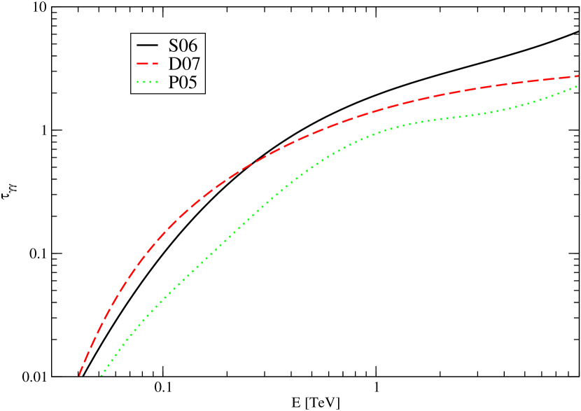
Figure 3: A comparison of the photoabsorption opacity for various IBL formulations for $z=0.116$, the redshift of PKS 2155–304.

Absorption by pair production will also occur due to interactions with the IBL (modifying the observed spectrum by a factor of $e^{-\tau_{\gamma\gamma}}$). In fact, IBL absorption is found to dominate the internal $\gamma\gamma$ absorption for the blazars considered here where we require large Doppler factors to produce hard-spectra multi-TeV emission. Formulas for absorption due to the IBL can be found in Stecker et al. (2006, hereafter S06), Stecker & Scully (2006), and Stecker et al. (2007). However, it has recently been pointed out that their approximations may overestimate the IBL (Dermer, 2007a, hereafter D07), which is more consistent with the calculations of Primack et al. (2005, hereafter P05); thus we use both the S06 and D07 formulations for $\tau_{\gamma\gamma}$ from the IBL. A comparison of the opacity from the IBL formulations of S06, D07, and P05 for PKS 2155–304 (catalog ) can be found in Fig. 3.

2.6 Jet Power and Constraints on $B$

The synchrotron emission implies a minimum total (particle and field) jet power, for a given Doppler factor, variability timescale, and magnetic field. The magnetic field which minimizes this jet power will be called $B_{min}$. Modeling the SSC component implies the departure of the magnetic field and jet power from these values.

We use the $\delta$-approximation to deduce the nonthermal electron spectrum from the synchrotron spectrum, from which the total nonthermal electron energy and nonthermal jet electron power can be derived. Adding the hadron and magnetic field energy gives a jet power that can be compared with the Eddington luminosity. The comoving energy in the magnetic field is given by

$$W^{\prime}_{B}=V_{b}^{\prime}U_{B}=\frac{R^{\prime 3}_{b}B^{2}}{6}\;,$$ (40)

while the total comoving energy in the electrons is given by

$$W^{\prime}_{e}=m_{e}c^{2}\int^{\gamma^{\prime}_{2}}_{\gamma^{\prime}_{1}}d\gamma^{\prime}_{s}\ \gamma^{\prime}_{s}\ N^{\prime}_{e}(\gamma^{\prime}_{s})\ .$$ (41)

Substituting the electron distribution, $N^{\prime}_{e}(\gamma^{\prime}_{s})$ from eq. (5) into eq. (41) and recalling eq. (4), $\gamma_{s}^{\prime 2}=\epsilon(1+z)/(\delta_{\rm D}\epsilon_{B})\ ,$ one obtains

$$W^{\prime}_{e}=m_{e}c^{2}\frac{6\pi d_{L}^{2}}{c\sigma_{T}\epsilon_{B}^{2}U_{Bcr}\delta_{\rm D}^{4}}\ \frac{1}{2}\ \sqrt{\frac{\delta_{\rm D}\epsilon_{B}}{1+z}}\ I_{syn}\;,$$ (42)

where

$$I_{syn}=\int_{\delta_{\rm D}\epsilon_{B}\gamma^{\prime}_{1}/(1+z)}^{\delta_{\rm D}\epsilon_{B}\gamma^{\prime}_{2}/(1+z)}d\epsilon\frac{f_{\epsilon}^{syn}}{\epsilon^{3/2}}\$$

and $U_{Bcr}=B_{cr}^{2}/(8\pi)$. Thermal protons or protons co-accelerated with electrons will also contribute to the total particle energy. The ratio of the total particle to electron energies is given by $\xi\equiv W^{\prime}_{par}/W_{e}^{\prime}$, so that the energy in all of the particles (electrons and protons) is

$$W^{\prime}_{par}\;=\;\xi W_{e}^{\prime}\;=\;\frac{3\pi d_{L}^{2}\xi m_{e}c^{2}}{c\sigma_{T}\epsilon_{B}^{3/2}(1+z)^{1/2}U_{Bcr}\delta_{\rm D}^{7/2}}\ I_{syn}\;.$$ (43)

In our calculations, we set $\xi=10$.

The total jet power in the stationary frame (i.e., the frame of the galaxy), is given by

$$P_{j}=2\pi R_{b}^{\prime 2}\beta\Gamma^{2}c\frac{W_{tot}^{\prime}}{V_{b}^{\prime}}$$ (44)

(Celotti & Fabian, 1993; Celotti et al., 2007), where $W^{\prime}_{tot}=W^{\prime}_{par}+W^{\prime}_{B}$, and the factor of 2 is due to the assumption that the black hole powers a two-sided jet. This formulation gives parameters that minimize black hole jet power (Dermer & Atoyan, 2004), though without taking into account whether these parameters provide a good spectral fit. The magnetic field that minimizes the jet power $P_{j}$is obtained by solving $|{dP_{j}/d\epsilon_{B}}|_{\epsilon_{B}=\epsilon_{B,min}}=0$ for $\epsilon_{B}=B/B_{cr}$. Doing this gives

$$\epsilon_{B,min}=\left[\left(\frac{3}{2}\right)^{3}\ \frac{\xi m_{e}c^{2}d_{L}^{2}(1+z)^{5/2}}{2t_{v,min}^{3}c^{4}\sigma_{\rm T}U_{Bcr}^{2}\delta_{\rm D}^{13/2}}\ I_{syn}\right]^{2/7}\ .$$ (45)

Smaller or larger magnetic field values than $B_{cr}\epsilon_{B,min}$ are possible, but only for more powerful jets. The minimum $P_{j}$ becomes

$$P_{j,min}=\frac{14}{3}\ \pi\;R_{b}^{\prime 2}\epsilon^{2}_{B,min}\beta\Gamma^{2}U_{Bcr}\;=\frac{14}{3}\ \pi c^{3}\left[\frac{\delta_{\rm D}\Gamma t_{v,min}\epsilon_{B,min}}{1+z}\right]^{2}\beta U_{Bcr}\;,$$ (46)

which makes the ratio of the jet power to the minimum jet power

$$\frac{P_{j}}{P_{j,min}}=\frac{3}{7}\left[\zeta_{B}^{2}+\frac{4}{3}\zeta_{B}^{-3/2}\right]\;,$$ (47)

where $\zeta_{B}=\epsilon_{B}/\epsilon_{B,min}$.

It is also useful to compare the jet power with the total luminosity, which is given by

$$L_{tot}\cong\frac{2\pi d_{L}^{2}}{\Gamma^{2}}\ \int_{0}^{\infty}d\epsilon\ \frac{f_{\epsilon}}{\epsilon},$$ (48)

including the beaming factor $1/2\Gamma^{2}$ for a two-sided jet. The radiative efficiency is given by $L_{tot}/P_{j}$.

2.7 Fitting Technique

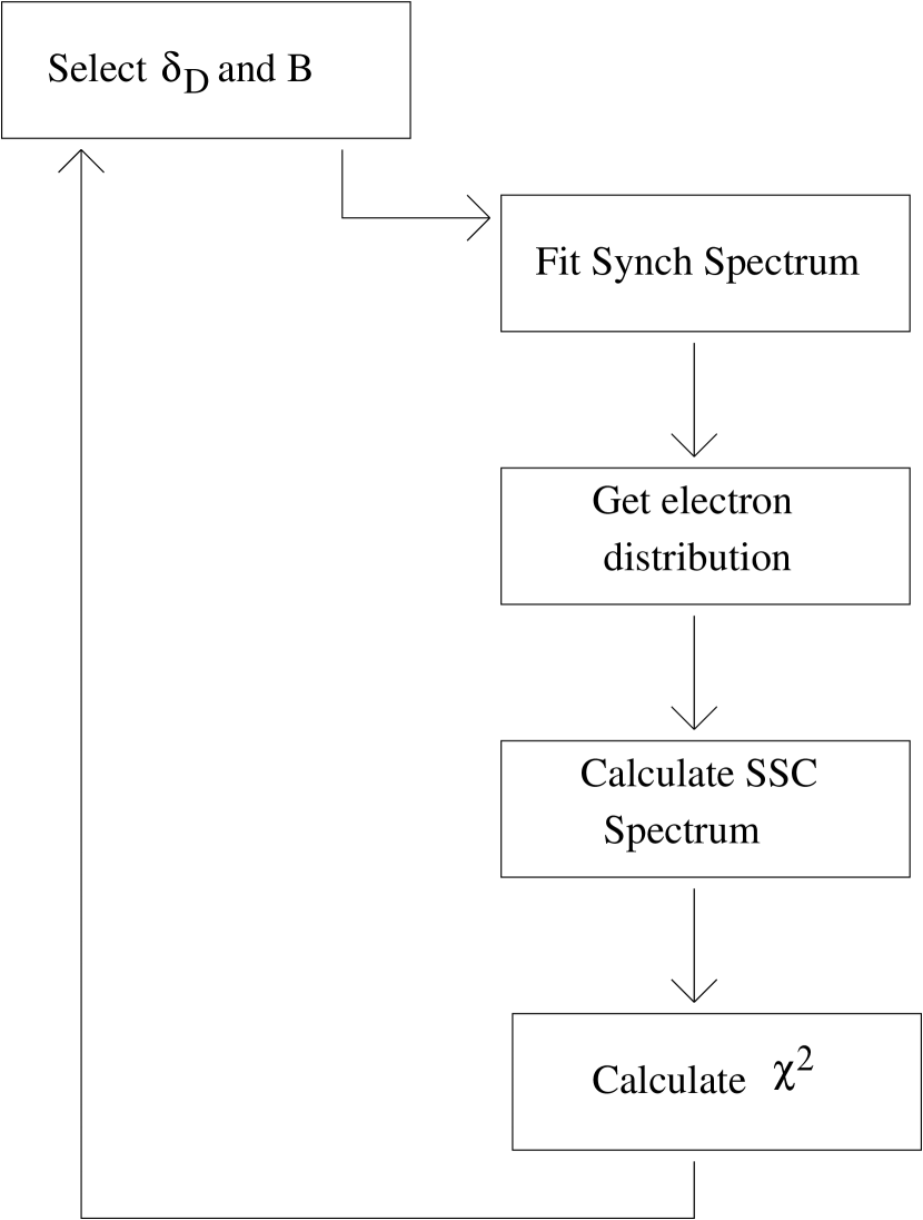
Figure 4: Diagram demonstrating the synchrotron and SSC fitting procedure.

We calculate the synchrotron spectrum with eq. (21) using a model for the comoving electron spectrum, and calculate the SSC spectrum with eq. (23) taking into account internal $\gamma\gamma$ absorption, eq. (32), and IBL $\gamma\gamma$ absorption. The synchrotron and SSC components are fit separately and iteratively in the following manner (see Fig. 4): Starting values are chosen for the electron distribution parameters (see § 3.1), $\delta_{\rm D}$ and $B$. The synchrotron spectrum calculated with eq. (21) is fit to the low energy (in this case, Swift) data points by varying the electron distribution but keeping $\delta_{\rm D}$ and $B$ constant, using a $\chi^{2}$ minimization technique (i.e., the Method of Steepest Descent; e.g., Press et al., 1992). Once the electron distribution is obtained from this fit, the high energy data are fit to the SSC component, calculated from eq. (23) and $\chi^{2}$ is calculated. Then the parameters $\delta_{\rm D}$ and $B$ are varied, the synchrotron spectrum is again fit to the low energy data to obtain the electron distribution, and another $\chi^{2}$ is calculated from the high energy data. This process is repeated until the parameters ($\delta_{\rm D}$ and $B$) that minimize $\chi^{2}$ are found. The constants of the problem are the multiwavelength spectral data, the source redshift $z$, variability timescale $t_{v,min}$, and the lower Lorentz factor $\gamma^{\prime}_{1}$ of the electron distribution.

In order to account for systematic errors in the VHE data, which usually dominates the measurement errors, we performed fits by multiplying the VHE data by a factor of $N_{sys}(\nu/\nu_{mid})^{a_{sys}}$ where $\nu_{mid}$ is the geometric mean of the VHE data, and $N_{sys}$ and $a_{sys}$ fit parameters that were allowed to vary within the systematic error range. $N_{sys}$ accounts for the normalization error, and $a_{sys}$ accounts for the spectral index error; for no systematic errors, $N_{sys}=1$ and $a_{sys}=0$.

3 APPLICATION TO PKS 2155–304

The XBL PKS 2155–304 (catalog ), an EGRET source (Hartman et al., 1999) and one of the brightest blazars at TeV energies, has been the subject of several multiwavelength campaigns (e.g., Zhang et al., 2006; Osterman et al., 2007; Sakamoto et al., 2007). The redshift of PKS 2155–304 (catalog ) is $z=0.116$ (Falomo et al., 1993; Sbarufatti et al., 2006), giving a luminosity distance of $d_{L}=540$ Mpc in a cosmology where $H_{0}=70$ km s^-1 Mpc^-1, $\Omega_{M}=0.3$, and $\Omega_{\Lambda}=0.7$.

In July and August of 2006, the source underwent several extremely bright flares which were detected by HESS (Aharonian et al., 2007a) and followed up by Swift (Benbow et al., 2006; Foschini et al., 2007). The measured variability timescales of the flares were as short as a few minutes with HESS. Swift’s observing schedule did not allow it to probe such small timescales; however, BeppoSAX observations from 1996 to 1999 show X-ray variability on scales of $\sim 1$ hour (Zhang et al., 2002). Preliminary analysis of Chandra data taken simultaneously with the HESS observations show them to be strongly correlated, and thus have X-ray variability timescales of a few minutes as well, although ground-based observations show the optical to be uncorrelated with the X-rays and VHE $\gamma$-rays (Costamante et al., 2007). Rapid variability does not seem to be intrinsic to only PKS 2155–304 (catalog ), as variability on timescales of a few minutes at TeV energies has been observed from Mkn 501 (catalog ) as well (Albert et al., 2007). The lack of optical correlation makes it unlikely that the optical emission came from the blob where the flare originated, and hence we consider the Swift optical data an upper limit.

The data used in our analysis are not simultaneous; the Swift ultraviolet/optical telescope (UVOT) and X-ray telescope (XRT) data are from 30 July, when it first observed the flares, while the HESS data are from 28 July. Detailed simultaneous HESS data have not yet been made available, although PKS 2155–304 (catalog ) was detected by HESS on 30 July simultaneously with the Swift detection (Foschini et al., 2007).

Using eqs. (21) and (23), and taking taking into account $\gamma\gamma$ absorption by internal jet radiation (eq. [32]) and the IBL, we simulate the broadband emission during one of these extremely bright flares. We fit the fully reduced Swift and HESS data, with the Swift data corrected by Foschini et al. (2007) for a Galactic column density of $N_{H}=1.36\times 10^{20}$ cm^-2.

3.1 The Electron distribution

The electron distribution is assumed to be of the form

$$N_{e}(\gamma^{\prime})=K_{e}\Biggr{[}\left(\frac{\gamma^{\prime}}{\gamma^{\prime}_{break}}\right)^{-p}H(\gamma^{\prime}_{break}-\gamma^{\prime})+$$ (49)

$$\left(\frac{\gamma^{\prime}}{\gamma^{\prime}_{break}}\right)^{-(p+1)}H(\gamma^{\prime}-\gamma^{\prime}_{break})\Biggr{]}H(\gamma^{\prime};\gamma^{\prime}_{1},\gamma^{\prime}_{2})\;.$$

As long as $\gamma^{\prime}_{1}\lesssim\gamma^{\prime}_{min}$ (eq. [13]) and $\gamma^{\prime}_{2}\gg\gamma^{\prime}_{c}$, the values of $\gamma^{\prime}_{1}$ and $\gamma^{\prime}_{2}$ do not affect our fits. This leaves us with four fitting parameters to define the electron spectrum, $K_{e}$, $p$, and $\gamma^{\prime}_{break}$. This spectrum is physically motivated, in that radiative cooling is expected to modify the electron power-law index by 1. For all of out fits to PKS 2155–304 (catalog ), we found $p=2.7$.

The electron distribution fitting parameters are not unique, and several sets of parameters give equally good fits to a given synchrotron spectrum. The fit of the SSC spectrum to the $\gamma$-ray data and the parameters $\delta_{\rm D}$ and $t_{v,min}$ derived in the fitting routine are, however, essentially independent of electron distribution parameters, as long as they provide a good fit to the synchrotron component.

3.2 The SSC Spectrum

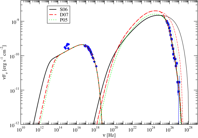
Figure 5: Various synchrotron and SSC fits for $t_{v,min}=300$ sec, for various IBL formulations. Swift UVOT and XRT data from PKS 2155–304 for 30 July 2006 (diamonds), as well as HESS data from 28 July 2006 (squares) are shown. The thin curves are the unabsorbed spectra, while the thick curves take into account $\gamma\gamma$ absorption by jet internal radiation and the IBL.

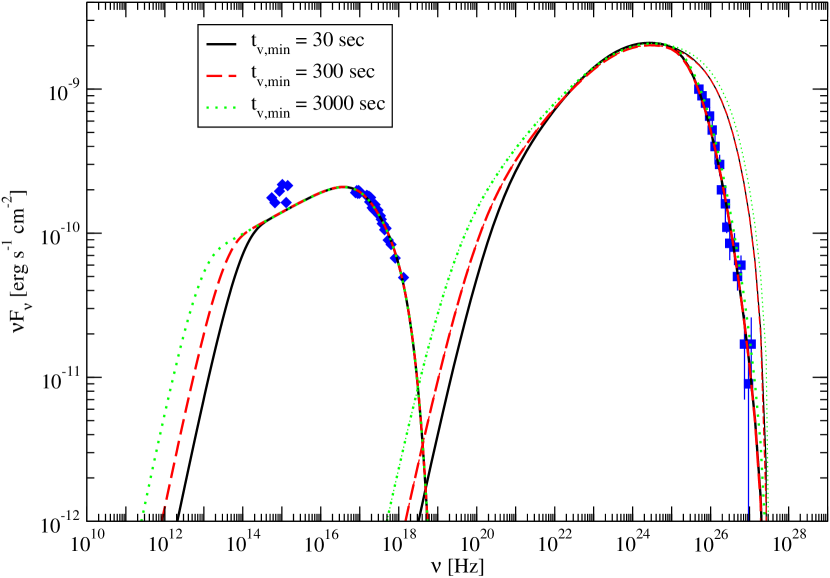
Figure 6: Similar to Fig. 5 figure compares models with different $t_{v,min}$ for the D07 IBL.

The Swift and HESS data from PKS 2155–304 (catalog ) were fit using the technique described in § 2.7. Results of the fits can be seen in Table 2 and in Figs. 5 and 6. The parameters $t_{v,min}$ and $\gamma^{\prime}_{1}$ were kept constant during the fits, and the angle along the line of sight was assumed to be small, so that $\Gamma\approx\delta_{\rm D}$ for the purpose of calculating the jet power. When we did vary $\gamma^{\prime}_{1}$, we found that this had no significant effect on our fits, as long as it was sufficiently low. All the models presented here have $\gamma^{\prime}_{1}=10^{3}$. Based on the systematic errors reported in Aharonian et al. (2007a), $N_{sys}$ was allowed to vary between 0.8 and 1.2, and $a_{sys}$ was allowed to vary between $-0.1$ and $+0.1$. This leads to the error bars on $\delta_{\rm D}$ and $B$ in Table 2, which are systematic error bars.

The fit parameters are strongly dependent on $t_{v,min}$. As $t_{v,min}$ increases, the best fit $\delta_{\rm D}$ decreases. This is mainly due to the relationship defining the SSC spectrum in eq. (17), which remains roughly constant provided that the quantity $t_{v,min}\delta_{\rm D}^{3}B$ remains constant, which is true for scattering in the Thomson regime, as shown below.

Based on the Swift and HESS data, eq. (39) gives the constraint

$$\delta_{\rm D}\gtrsim 48\left(\frac{300\ \sec}{t_{v,min}}\right)^{0.175}\ .$$ (50)

Thus, the short variability in PKS 2155-304 (catalog ) ($\approx 300$ sec, Aharonian et al., 2007a) limits the Doppler factor to quite high values (see also Begelman et al., 2008). Another constraint can be found from eq. (28) by noting that the peak energy for the SSC component must be $>0.2$ TeV ($\epsilon_{s}>4\times 10^{5}$). This leads to

$$\left(\frac{B}{1\ \textrm{G}}\right)\delta_{\rm D}\gtrsim 7$$ (51)

(Tavecchio et al., 1998; Bednarek & Protheroe, 1997, 1999).

The best fit magnetic field values implied by spectral modeling are a few to $\approx 100\$ mG, which represent a small fraction of the magnetic field, eq. (45), that minimizes the jet power. The absolute jet powers for a two-sided jet derived from these fits are $\approx 10^{46}$ – $10^{47}$ ergs s^-1, representing a very large fraction of the Eddington luminosity for a $10^{9}M_{\odot}$ black hole ($L_{Edd}=1.3\times 10^{47}$ erg s^-1). Values this large would cast doubt on the underlying one-zone synchrotron/SSC and IBL model. Also note that the small values of $\zeta_{B}$ indicates that $W^{\prime}_{par}\gg W^{\prime}_{B}$; thus, $P_{j}\propto\xi$, and if $\xi$ is any larger, the jet power will be larger by the same factor. Because the jet power is strongly particle-dominated, it is very dependent on the value of $\gamma^{\prime}_{1}$, which is not strongly constrained by our models. However, we take $\gamma^{\prime}_{1}=10^{3}$, a rather large value. It is unlikely to be larger, and thus, the jet power is unlikely to be lower, although this part of the electron distribution is not well-constrained by observations due to the lack of correlated optical variability. Our choice of electron spectral index assumes the blob is primarily cooled by synchrotron or SSC emission, which may not be the case (see below).

Fits were performed with the IBL models of (in order of decreasing intensity) S06, D07, and P05. The lower-intensity IBLs do lower the Doppler factors and jet powers considerably. This may be an arguement for the lower IBLs, which has also been suggested from observations of TeV observations of 1ES 1101–232 (Aharonian et al., 2006) and 1ES 0229+200 (Aharonian et al., 2007b). However, the jet powers are still quite large compared to the probable Eddington limit. The lowest Doppler factor we were able to obtain, with the lowest IBL and longest $t_{v,min}$ was $\delta_{\rm D}=58$. This Doppler factor is still considerably larger than values measured with the VLBA from PKS 2155–304 (catalog ) on the parsec scale ($\beta_{obs}\sim 4$; Piner & Edwards, 2004). The $\gamma$-ray emission may, however, be formed on size scales that are tens to hundreds of times smaller. Note that the models differ significantly in the frequency region that GLAST will observe (i.e., $\sim 10$ MeV—100 GeV); thus, GLAST will be quite useful for distinguishing between models.

3.3 Temporal Variability

Temporal variability can result from acceleration, adiabatic expansion, and radiative cooling. Nonthermal electrons that cause blazar flares are thought to be accelerated to high energies by a Fermi acceleration mechanism, possibly caused by internal shocks in the collision of irregularities in the relativistic jetted wind. The particle acceleration timescale in the comoving frame for a Fermi mechanism is

$$t_{acc}^{\prime}=N_{a}\ \frac{\gamma^{\prime}}{\nu_{B}}$$ (52)

where $N_{a}\gtrsim 1$ is the number of gyrations an electron makes while doubling its energy, and

$$\nu_{B}=\frac{eB}{2\pi m_{e}c}\$$

is the Larmor frequency (e.g., Gaisser, 1990).

As the electrons radiate synchrotron and Compton-scattered radiation, they lose energy. The electron energy-loss rate, or cooling rate, in the comoving frame from synchrotron radiation is

$$-\dot{\gamma^{\prime}}_{syn}=\frac{4}{3}c\sigma_{\rm T}u_{B}\gamma^{\prime 2}.$$ (53)

The SSC cooling rate using the full Klein-Nishina cross section (Jones, 1968; Böttcher et al., 1997) is

$$-\dot{\gamma^{\prime}}_{SSC}=\frac{3\sigma_{\rm T}}{8m_{e}c}\int^{\infty}_{0}d\epsilon^{\prime}\frac{u^{\prime}(\epsilon^{\prime})}{\epsilon^{\prime 2}}\ G(\gamma^{\prime}\epsilon^{\prime})$$ (54)

where

$$G(E)=\frac{8}{3}E\frac{1+5E}{(1+4E)^{2}}\ -\ \frac{4E}{1+4E}\left(\frac{2}{3}+\frac{1}{2E}+\frac{1}{8E^{2}}\right)$$

$$+\ \ln(1+4E)\left(1+\frac{3}{E}+\frac{3}{4}\frac{1}{E^{2}}+\frac{\ln[1+4E]}{2E}-\frac{\ln[4E]}{E}\right)$$

$$-\ \frac{5}{2}\frac{1}{E}\ +\ \frac{1}{E}\sum^{\infty}_{n=1}\frac{(1+4E)^{-n}}{n^{2}}\ -\ \frac{\pi^{2}}{6E}\ -\ 2\;,$$ (55)

and $u^{\prime}(\epsilon^{\prime})$ is the synchrotron spectral energy density, given by eq. (8). With these expressions one can determine the cooling timescales in the observer’s frame, given by

$$t_{cool}\ =\ \frac{1+z}{\delta_{\rm D}}\ t^{\prime}_{cool}\ =\ \frac{1+z}{\delta_{\rm D}}\ \vline\frac{\gamma^{\prime}}{\dot{\gamma}^{\prime}}\vline\ .$$ (56)

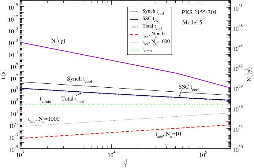
Figure 7: The cooling timescales for synchrotron (thin solid black curve) and SSC (thick solid black curve) as a function of electron energy for Model 5. The total cooling time from both of these processes is plotted as a dashed-dotted blue curve. The acceleration timescale is plotted as the dashed red and brown curves with $N_{a}=10$ and $N_{a}=1000$, respectively, and the variability timescale for this simulation (300 s) is shown as the dotted green curve. Also overplotted is the form of the electron spectrum, $N_{e}^{\prime}(\gamma^{\prime})$ (solid violet curve).

The acceleration and cooling timescales can be seen in Fig. 7 for Model 3 with $t_{v,min}=$ 300 s and $N_{a}=10$ and 1000; results for other models are similar. The SSC cooling timescale starts to deviate from the Thomson regime behavior at $\gamma^{\prime}\gtrsim 2\times 10^{5}$ due to Klein-Nishina effects, which is not seen on this plot. Overplotted on this graph is the electron spectrum used to fit the PKS 2155–304 (catalog ) data, which cuts off at $\gamma^{\prime}=2\times 10^{5}$. In PKS 2155–304 (catalog ), the cutoff in the synchrotron spectrum at $\nu\approx 10^{18}$ Hz means that electrons are not accelerated to extremely large Lorentz factors. If the cutoff in the synchrotron spectrum and therefore the electron spectrum is attributed to cooling that prevents acceleration to higher energies, then $N_{a}$ must be very large, $\gtrsim 10^{5}$. This could occur if there are more severe limitations to electron acceleration than implied by the simple expression given by eq. (52). See § 5 for further discussion.

4 APPLICATION TO MKN 421

The XBL Mkn 421 (catalog )—the first blazar seen at TeV energies—has been the target of many multiwavelength campaigns (e.g., Macomb et al., 1995; Fossati et al., 2004, 2008). The campaign of March 2001 was one of the longest and most complete (Fossati et al., 2008), in which it was observed by RXTE, Whipple, HEGRA, and the Mt. Hopkins 48″ telescope nearly continuously for seven days. During this campaign on 19 March 2001, an extremely bright flare was observed with all three instruments. In this section, we model this flare with our SSC methodology. Mkn 421 (catalog ) has shown variability on timescales down to $\sim 1000$ s (e.g., Aharonian et al., 2002). This XBL has a redshift of $z=0.03$ (Ulrich et al., 1975; Ulrich, 1978) giving it a luminosity distance of $d_{L}=130$ Mpc using the cosmological parameters mentioned in § 3.

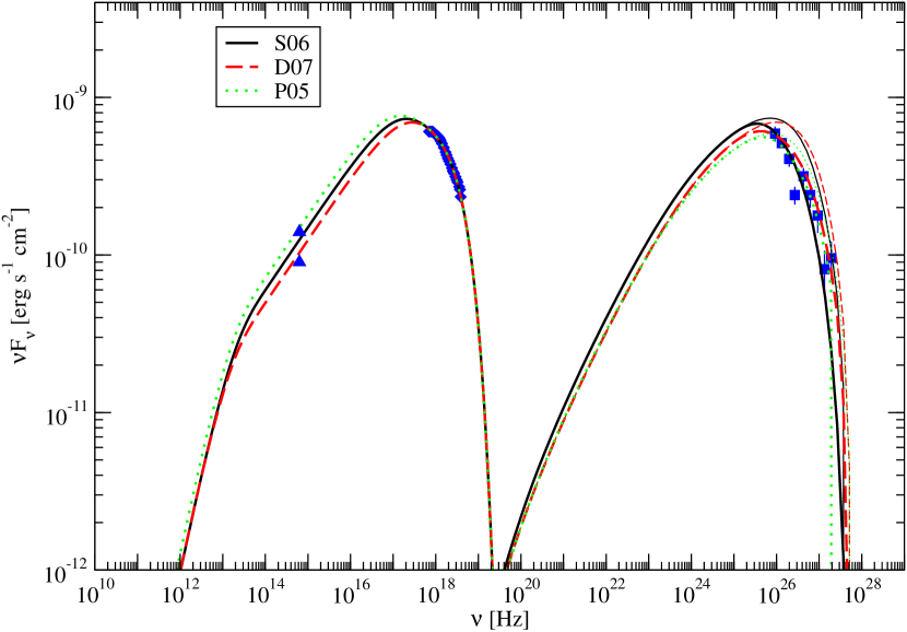
Figure 8: Synchrotron SSC model fits to the March 2001 flare observed by Fossati et al. (2008) in Mkn 421 for $t_{v,min}=10^{3}$ sec. The triangles are limits from the Hopkins 48″ optical observations, the diamonds are the RXTE data, and the squares are the HEGRA data (Aharonian et al., 2002). The thin curves are the unabsorbed spectra, while the thick curves take into account $\gamma\gamma$ absorption by jet internal radiation and the IBL.

Fits to the March 2001 flare for different $t_{v,min}$ and IBL formulations are shown in Table 3 and Fig. 8. We fit to the fully reduced data from Fossati et al. (2008). The RXTE data was reduced assumed a Galactic column density of $1.6\times 10^{20}$ cm^-2, although this makes little difference for RXTE’s bandpass. The same electron distribution as for PKS 2155–304 (catalog ) was used, namely eq. (49), except for Mkn 421 (catalog ), the best fit electron power-law index was $p=2.2$. Again, it is assumed $\delta_{\rm D}\approx\Gamma$.

As with PKS 2155–304 (catalog ), for a constant $t_{v,min}$, as $\delta_{\rm D}$ increases, $B$ decreases. The opacity constraint, eq. (39), gives

$$\delta_{\rm D}\gtrsim 29\left(\frac{10^{3}\ \sec}{t_{v,min}}\right)^{0.2}\ .$$ (57)

The S06 and D07 IBLs are nearly identical for $z=0.04$. All IBLs result in a low opacity of intergalactic space at such low $z$. Absorption by the IBL plays a small, but non-negligable part for low-$z$ VHE $\gamma$-ray sources. However, the difference between the IBL formulations is negligible, as the solutions with different IBLs are all within the margin of error.

The model fits of Fossati et al. (2008) give $\delta_{\rm D}=100$ and $B=1$ G for a blob size of $R_{b}^{\prime}=1\times 10^{14}$ cm which is similar to our fits, except with a larger $B$. It should be noted that their models do not fit the TeV data particularly well. VLBA observations of Mkn 421 (catalog ) show only weak superluminal motion, with $\beta_{obs}\sim 0.1$ on parsec scales (Piner & Edwards, 2005). As with PKS 2155-304 (catalog ), the jet must slow down considerably from the $\gamma$-ray emitting region to the parsec-scale jet. Also as before, $\zeta_{B}$ is very similar in all fits.

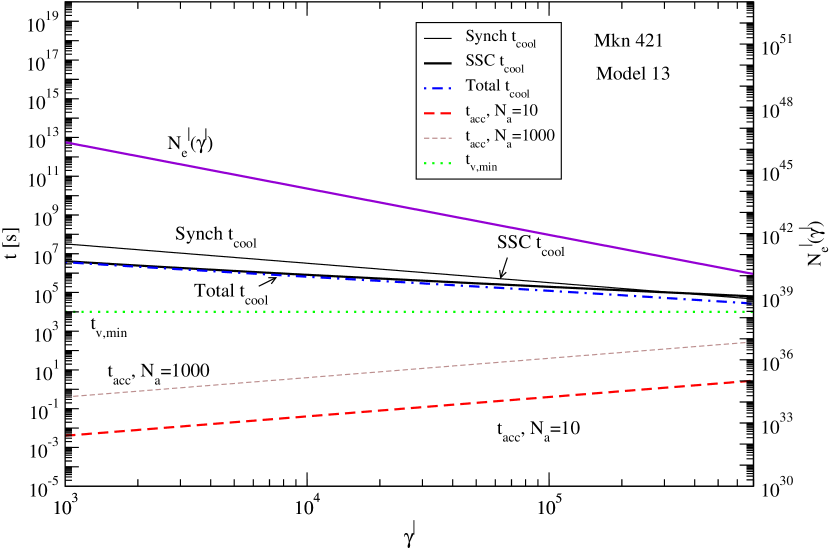
Figure 9: Similar to Fig. 7 only for Model 13 of Mkn 421.

The cooling timescales for Model 13 for Mkn 421 can be seen in Fig. 9. Here, the Klein-Nishina effects on the Compton cooling timescale are visible at $\gamma^{\prime}\sim 8\times 10^{4}$, indicating that accounting for Klein-Nishina effects is quite important for modeling this flare. As with PKS 2155–304 (catalog ), the cooling timescale is longer than the variability timescale, which poses problems for the SSC model.

5 DISCUSSION

We have presented a new approach to modeling XBL radiation in a synchrotron/SSC framework. We obtain the electron spectrum by fitting a model nonthermal electron distribution to the low energy radio/optical/X-ray data, assuming that it arises from nonthermal synchrotron processes. This electron spectrum is then used to calculate the SSC component and to fit the $\gamma$-ray data as a function of a small set of parameters. The number of free parameters, namely the Doppler factor, magnetic field, and size scale of the radiating region, is small enough that $\chi^{2}$ fits can be performed to high quality multiwavelength data. We discuss the results given by fitting the non-simultaneous PKS 2155–304 (catalog ) data (keeping in mind that unambiguous conclusions will require simultaneous data sets), as well as simultaneous M (catalog )kn 421 data.

5.1 The Rapid Flare in PKS 2155–304

For the giant flare in PKS 2155–304 (catalog ), the rapid ($\sim 5$ min) variability implies a small emitting region. This creates problems for the one-zone SSC model for three main reasons: it requires excessively large Doppler factors, jet powers, and cooling timescales.

For fits to the full optical/UV/X-ray spectra for PKS 2155–304 (catalog ), we find that very large Doppler factors ( $\delta_{\rm D}\gtrsim 60$ for PKS 2155–304 (catalog )) are necessary to explain high energy emission with the SSC mechanism (similar to the findings of Begelman et al., 2008). However, radio measurements of superluminal motion from PKS 2155–304 (catalog ) indicate that the jet Lorentz factor $\Gamma\sim 10$, at least on parsec scales (Piner & Edwards, 2004). The cause of this discrepancy could be that the flare radiation is produced very close to the black hole, and that the blobs seen in the radio have slowed down before reaching parsec scales. However, a deceleration episode between the inner regions near the black hole and the parsec-scale region would likely produce observable high energy radiation distinct from the SSC component (e.g., Georganopoulos & Kazanas, 2003; Levinson, 2007). If all blazars have such large Doppler factors, the number of blazars aligned with our line of sight becomes smaller than the number actually observed.

The excessive jet powers required by our fits to the full optical/UV/X-ray and $\gamma$-ray spectra are another problem for the one-zone SSC model. The jet powers for PKS 2155–304 (catalog ) range from $\sim 10^{46}$ – $4\times 10^{47}$ ergs s^-1 (see Table 2); these powers can be reduced by a factor of 10 for a hadron-free pair jet, recalling that we assumed $\xi=10$. The higher values exceed the Eddington luminosity for a $\sim 10^{9}\ M_{\odot}$ black hole by a factor of a few. Even if the black hole exceeded $10^{9}M_{\odot}$, it is unlikely that a black hole with a jet would be so radiatively efficient. Large Doppler factors in synchrotron/SSC modeling were also found in analyses of Mkn 501 (catalog ) by Krawczynski et al. (2002).

The jet powers of our fits are significantly larger than the jet power, $6\times 10^{43}$ ergs s^-1, found for the SSC fit to the same PKS 2155–304 (catalog ) data by Ghisellini & Tavecchio (2008). Their SSC fit is closest to our Model 5, which underfit the optical Swift data as well. The electron jet power in Model 5 is a factor of $\sim 40$ times larger than the SSC model of Ghisellini & Tavecchio (2008), when taking into account the fact that they calculated it for a one-sided jet. The main reason for this is that their synchrotron component underfits the optical data by a larger amount (also note that they did not use the full Compton cross-section, which can significantly affect derived parameter values and jet powers; see § 2.4). Even though the bolometric power at optical energies is only a factor of $\sim 3$ greater than the X-ray power, the total jet power in a synchrotron/SSC model that fits the optical as well as the X-rays is much greater than the power to fit the X-ray and TeV radiation because of the many low-energy radiatively inefficient electrons required to emit the lower energy optical radiation in the spectrum. It is also worth reminding the reader that, as discussed in § 3.2, the low energy part of the electron distribution—and hence the jet power— is essentially unconstrained by optical observations. However, it is difficult to imagine how $\gamma^{\prime}_{1}$ could be much larger than $10^{3}$, so that our jet powers could be considered lower limits. Our jet powers are also dependent on the assumption of cooling dominated by synchrotron or SSC losses.

Another important issue for the SSC model studied here is that one would expect the timescale of variability at X-ray synchrotron and TeV $\gamma$-ray energies generated by the same electrons would be approximately equal. Equating eqs. (4) and (26), assuming that the high-energy radiation is dominated by Thomson-scattered peak synchrotron photons with energy $\epsilon_{pk}$, implies that photons with energy $\epsilon_{s}\cong(1+z)\epsilon_{pk}\epsilon_{syn}/(\delta_{\rm D}\epsilon_{B})$ (eq. [28]) are produced by the same electrons that emit synchrotron radiation with energies $\sim\epsilon_{syn}$. The results of Model 3 for PKS 2155–304 (catalog ) in Table 2 imply that $\epsilon_{s}\cong 3.3\times 10^{9}\epsilon_{syn}$, taking $\epsilon_{pk}\cong 10^{-4}$. Electrons Compton scattering $\epsilon_{pk}$ photons to make 1 TeV photons would therefore be radiating synchrotron photons at $\approx 0.3$ keV with the same short variability timescale as measured at TeV energies. Because the SSC cooling timescale in the Thomson regime scales as $\propto\gamma^{\prime-1}$, the higher energy photons observed by Swift’s XRT should have an even shorter variability timescale than observed at 1 TeV by HESS; however, Swift’s limited observing schedule did not allow a detailed variability study. Chandra did observe the flare, and preliminary analysis seems to indicate the X-rays are highly correlated with the $\gamma$-rays observed by HESS (Costamante et al., 2007), and strong X-ray/$\gamma$-ray correlation in other blazar flares has been observed before (e.g., Fossati et al., 2008; Sambruna et al., 2000; Tavecchio et al., 2001), but its variability timescale is still not clear. In any case, whatever the source of the variability is, the timescale will be limited by the size scale of the emitting region.

The one-zone SSC model for the TeV flare in PKS 2155–304 (catalog ) implies, from Fig. 7, that the radiative cooling timescales are much longer than $t_{v,min}$. Thus, variability cannot be attributed to radiative cooling, but could originate from adiabatic expansion; however, as mentioned above, the lack of achromatic variability in PKS 2155-304 (catalog ) makes this seem unlikely. Thus, the variability is not consistent with the one zone synchrotron/SSC model. Begelman et al. (2008) use analytic estimates to show that, with the brightness and temporal variability observed in PKS 2155–304 (catalog ), $\Gamma\gtrsim 50$ for the radiation to avoid photoabsorption. They also suggest that magnetic energy density must dominate the jet power in order for the acceleration to be efficient, which limits $\Gamma\lesssim 40$; thus, the SSC model cannot explain these flares (however, in our simulations, the jet power is dominated by particle energy density [§ 3.2]). They suggest the flare is caused by Compton scattering of an external radiation field that must be limited to below sub-mm wavelengths. Using their inferred energy density for the external scattering radiation, then unless the size scale of this region is $\lesssim 3\times 10^{16}$ cm, this radiation should be observable, which makes it more likely to originate from an accretion disk.

Are there explanations that could resolve these issues with the rapid TeV flare from PKS 2155–304 (catalog )? We discuss three possibilites: external Compton scattering, relaxing the assumption of homogeneity, and lower IBL energy densities.

The SSC mechanism involving isotropic scattering is unable to decelerate a jet blob from the excessive Doppler factors found from our fits, to the Doppler factors required from radio observations (Piner & Edwards, 2005). Jet deceleration would require another mechanism such as external Compton scattering where jet electrons upscatter photons of an external radiation field. This would produce flares at GeV energies. These photons could originate from a slower-moving sheath surrounding a faster jet spine (Ghisellini et al., 2005; Tavecchio & Ghisellini, 2008), or from an advanced portion of the jet moving at a slower speed (Georganopoulos & Kazanas, 2003). The external photons would also serve as a power and cooling source, which could also resolve issues with excessive jet powers and cooling timescales. A complete analysis would require an extension of the synchrotron/SSC model to include external Compton scattering and effects of the $\gamma\gamma$ opacity (Reimer, 2007) from the scattered radiation field to account for the full broadband SED (C. D. Dermer, J. D. Finke, H. Krug, & M. Böttcher 2008, in preparation). In this case, the 100 GeV – TeV radiation would still predominantly arise from the SSC process because of strong Klein-Nishina effects on external Compton components from scattered optical/UV radiation, but the additional $\gamma\gamma$ opacity would have to be considered in the analysis.

Another possible explanation for the extreme parameters is that the homogeneous assumption for the blob is invalid. We have assumed that the synchrotron radiation, which provides target photons for Compton scattering, is emitted by the same nonthermal electrons, whereas they could originate from a more extended region. The correlated variability between X-rays and TeV $\gamma$-rays seen in PKS 2155-304 (Foschini et al., 2007; Costamante et al., 2007) indicate however that at least the higher energy synchrotron photons are probably co-spatially produced with the SSC radiation. Even in a one-zone model, the electrons could be strongly cooled before the synchrotron photons uniformly fill the emission region. Alternately, the entire blob might not be optically thin to $\gamma\gamma$ attenuation and the observed SSC emission may be from a smaller region than the synchrotron emission. Simulations with corrections to the one-zone approximation are necessary to investigate these possibilities.

Recent blazar observations may indicate an IBL energy density only slightly above the lower limits implied from galaxy counts (Aharonian et al., 2006, 2007b). The lowest IBL considered here, P05, gives significantly lower jet powers and Doppler factors for the PKS 2155–304 (catalog ) flare than the other models, which may be a further arguement for a lower IBL. The IBLs of D07 and P05 both give jet powers below the Eddington limit for a $10^{9}\ M_{\sun}$ black hole. However, the Doppler factors are still excessive.

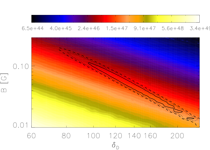
Figure 10: A plot of the jet power as a function of the parameters $\delta_{\rm D}$ and $B$ for Model 5. The color corresponding to a specific jet power is given in the bar above, in erg s^-1. Overplotted are the 68% (solid curve), 95% (dotted curve) and 99% (dashed curve) confidence contours for Model 5.

To determine how certain our fit from Model 5 is, we plotted the 68%, 95%, and 99% statistical uncertainty contours. Also plotted is the jet power as a function of the parameters $\delta_{\rm D}$ and $B$ for Model 5 in Fig. 10. The confidence contours trace a region that is roughly constant in terms of jet power; inside the 68% contour, the power varies between a relatively small amount (between roughly $2\times 10^{46}$ and $10^{47}$ erg s^-1). Also of note is that a relatively large range of Doppler factors ($\delta_{\rm D}\sim$ 80 – 170 with 68% confidence) will give a satisfactory fit. Even the lowest Doppler factors allowed are quite high. The Doppler factors are too high for the eq. (50) constraint to play a part. The lines of constant jet power follow a power law based on $B\propto\delta_{\rm D}^{-1.5}$, as one can see from eq. (44),

$$P_{j}\propto R_{b}^{\prime-1}\delta_{\rm D}^{2}W^{\prime}_{par}\ \propto\delta_{\rm D}W^{\prime}_{par}\ ,$$

if $\delta_{\rm D}\approx\Gamma$ and $W^{\prime}_{e}\gg W^{\prime}_{B}$. Most of the electron energy is located in the part of the electron spectrum below the break. Given a $\nu F_{\nu}$ spectral index of $a_{1}$ ($f_{e}\propto\epsilon^{a_{1}}$), and performing the integral in eq. (43), $W_{par}=B^{a_{1}-2}\delta_{\rm D}^{a_{1}-4}$. For constant $P_{j}$, this gives $B\propto\delta_{\rm D}^{\frac{a_{1}-3}{2-a_{1}}}$. For our fits to PKS 2155–304, $a_{1}=0.15$, and we recover $B\propto\delta_{\rm D}^{-1.5}$. Statistical uncertainty contours follow $B\propto\delta_{\rm D}^{-2.4}$, rather than the expected $B\propto\delta_{\rm D}^{-3}$ (§ 2.4). This is due to the fact that scattering occurs in the Klein-Nishina regime. For $\gamma^{\prime}\epsilon^{\prime}\gtrsim 1/4$, to zeroth order the scattering cross-section goes as approximately $\sigma_{KN}\propto\epsilon^{-1}$. At the peak energy, eq. (LABEL:festhom), using the Klein-Nishina cross section and eq. (28) becomes

$$f_{\epsilon^{pk}_{s}}^{SSC}\propto\frac{\left[f_{\epsilon}^{syn}(\epsilon^{pk}_{syn})\right]^{2}}{B^{2}\delta_{\rm D}^{6}\epsilon_{syn}^{pk}}\propto\frac{\left[f_{\epsilon}^{syn}(\epsilon^{pk}_{syn})\right]^{2}}{B^{5/2}\delta_{\rm D}^{13/2}}\ ,$$

which leads to $B\propto\delta_{\rm D}^{-2.6}$. This is very close to the $B\propto\delta_{\rm D}^{-2.4}$, considering the accuracy of the approximation. The internal $\gamma\gamma$ opacity, eq. (50), does not significantly constrain the Doppler factor in Fig. 10.

5.2 The March 2001 Flare in Mkn 421

For Mkn 421 (catalog ), we find $\delta_{\rm D}\gtrsim 30$ for our model fits. VLBA observations of Mkn 421 (catalog ) show only weak superluminal motion, with $\Gamma\sim 2$ on parsec scales (Piner & Edwards, 2005). Jet powers are one the order of $P_{j}\gtrsim 3\times 10^{45}$ erg s^-1, and for all of our models they do not exceed the Eddington luminosity for a $10^{9}$ M_☉ black hole. The parameters for this flare in Mkn 421 (catalog ) are thus much more reasonable than for PKS 2155–304 (catalog ). Fossati et al. (2008) found the X-rays and VHE $\gamma$-rays to be highly correlated, indicating that they are likely emitted from the same part of the jet, although a highly variable external X-ray source that is Compton scattered by a blob would also explain this. As seen in Fig. 9, the cooling timescale is significantly longer than the variability timescale, as with the PKS 2155–304 (catalog ) flare. Thus the variability discussion in the previous section applies to Mkn 421 (catalog ) as well, and it is possible that Mkn 421’s variability is dominated by some other mechanism. Analysis of hardness-intensity diagrams could indicate the effects of additional radiation mechanisms or variability sources (e.g., Kataoka et al., 2000; Li & Kusunose, 2000; Böttcher & Chiang, 2002). For example, if adiabatic expansion dominates the energy-loss rate of electrons with sufficiently low Lorentz factors, then the corresponding achromatic synchrotron spectral variability should allow one to distinguish this from frequency-dependent radiative cooling effects.

5.3 Predictions for GLAST

Fig. 11 shows the blazar $\nu F_{\nu}$ flux that would be significantly detected with GLAST in the scanning mode as a function of observing time (see Appendix A). The predicted fluxes of PKS 2155–304 (catalog ) shown in Figs. 5 – 6 have a $\nu F_{\nu}$ flux at 1 GeV of $\approx 8\times 10^{-10}$ ergs cm^-2 s^-1 and a $\nu F_{\nu}$ spectral index $a=0.5$. From Fig. 11, we see that GLAST will significantly detect PKS 2155–304 (catalog ) at this flux level in less than one or two ksec when integrating above $100$ MeV, and $\lesssim 10$ ksec when integrating above 1 GeV. Significant detection of Mkn 421 (catalog ) will be achieved with GLAST in $\lesssim 30$ ksec whether integrating above 100 MeV or 1 GeV, as can be seen from Fig. 8. For PKS 2155–304 (catalog ), the predicted $\nu F_{\nu}$ flux is quite sensitive to the assumed IBL (see Fig. 5), so if the synchrotron/SSC model is valid, then the different IBLs could in principle be distinguished.

5.4 Summary

We have modeled flares in PKS 2155–304 (catalog ) and Mkn 421 (catalog ) with a synchrotron/SSC model. Due to the high Doppler factors, jet powers, and radiative cooling timescales, we find that it is unlikely that SSC emission alone can explain the giant TeV flares in the blazar PKS 2155–304 (catalog ), at least for the one-zone approximation. Lowering the IBL energy density lowers these quantities considerably, but not enough to change our conclusions. Although one-zone SSC modeling of the March 2001 Mkn 421 (catalog ) flare gives reasonable jet powers and Doppler factors, the long cooling timescales cause problems for this flare as well. Compton scattering of photons from an external radiation source, for example, from radiation produced in different regions of the jet, or loosening the one-zone approximation, might remedy these problems. The addition of external scattered radiation to this analysis technique will be the subject of future work.

Appendix A GLAST Sensitivity to Blazar Flares

GLAST Large Area Telescope (LAT) sensitivity estimates to blazar flares are updated using the latest GLAST LAT performance parameters. Let $u=E$(GeV) represent photon energy in GeV. The effective area of the GLAST LAT, accurate to better than 15% for 70 MeV $\lesssim E\lesssim 200$ GeV, can be written as

$$A(u)=A_{0}\cases{\sqrt{u},&$0.07\lesssim u\lesssim 1$\cr 1,&if $1\lesssim u\lesssim 200$,\cr}$$ (A1)

with $A_{0}=8600$ cm². Following the approach of Dermer (2007b), the number of source counts detected with the GLAST LAT above photon energy $u$ GeV is

$$S(>u)={\eta_{\gamma}X\Delta tf_{GeV}A_{0}\over E_{GeV}}\;\left\{{2(u^{a-1/2}-1)H(1-u)\over 1-2a}+{[\max(1,u)]^{a-1}\over{1-a}}\right\}\;.$$ (A2)

Here $\Delta t$ is the total observing time and $X$ is the occultation factor in the scanning mode, $\eta_{\gamma}=0.67$ is an acceptance cone about the source, and $E_{GeV}=1.6\times 10^{-3}$ ergs is 1 GeV in units of ergs, provided that the blazar $\nu F_{\nu}$ spectrum $f_{\epsilon}$ is given in units of ergs cm^-2 s^-1. The blazar flare spectrum is assumed to be described by a single power law with $\nu F_{\nu}$ index $a$, so that $f_{\epsilon}=f_{\rm GeV}u^{a}H(u;u_{1},u_{2})$, where $f_{GeV}$ is the $\nu F_{\nu}$ flux at 1 GeV, and the endpoints $u_{1}<0.07$ and $u_{2}\gtrsim 200$.

The GLAST LAT point spread function is given in terms of the angle $\theta(^{\circ})=0.62u^{-3/4}$ for 68% containment, and is accurate to better than 20% for $0.03<u<40$. The energy-dependent solid angle corresponding to this point spread function is therefore $\Delta\Omega(u)=\pi\theta^{2}=3.7\times 10^{-4}u^{-3/2}\equiv\omega_{0}u^{-3/2}$ sr. The number of background counts with energy $>u$ GeV is

$$B(>u)=A_{0}X\Delta tk_{\gamma}\omega_{0}\left\{\left({u_{1}^{-\alpha_{\gamma}-1}\over\alpha_{\gamma}}\right)H(1-u)+{\;2[\max(1,u)]^{-(\alpha_{\gamma}+0.5)}\over 1+2\alpha_{\gamma}}\;\right\}\;,$$ (A3)

using the diffuse $\gamma$-ray background measured with EGRET (Sreekumar et al., 1998) with photon index $\alpha_{\gamma}=2.10$ and coefficient $k_{\gamma}=1.37\times 10^{-6}$ ph/(cm²-s-sr).

Fig. 11 shows how bright the $\nu F_{\nu}$ flux has to be for GLAST to detect at least 5 counts and at $n=5$ $\sigma$ detection, estimated through the relation $n=S(>u)/\sqrt{2B(>u)}$ for $u=0.1$ and $u=1$, corresponding to $E>100$ MeV and $E>1$ GeV, respectively. Results are shown for a flat, $a=0$, and rising, $a=1/2$, $\nu F_{\nu}$ spectrum with $X=0.2$. The right-hand axis shows the corresponding integral photon flux for the $u>0.1$, $a=0$ case in units of $10^{-8}$ ph$(>100$ MeV)/(cm²-s). The break in these curves represents a transition from a signal-dominated, bright flux regime where the detection sensitivity $\propto\Delta t$ to a background-dominated, dim flux regime where the detection sensitivity $\propto\sqrt{\Delta t}$.

Table 1: Coefficients for the approximation to $R(x)$.

Coefficient	$10^{-2}<x<10^{0}$	$10^{0}<x<10^{1}$
$A_{0}$	-0.35775237	-0.35842494
$A_{1}$	-0.83695385	-0.79652041
$A_{2}$	-1.1449608	-1.6113032
$A_{3}$	-0.68137283	0.26055213
$A_{4}$	-0.22754737	-1.6979017
$A_{5}$	-0.031967334	0.032955035

Table 2: Parameters giving best fit SSC spectra to PKS 2155–304 data for different values of $t_{var}$ and IBL. See text for details.

Model No.	IBL	$t_{v,min}$	$\delta_{D}$	$B$	$\zeta_{B}$	$P_{j}$	$\frac{P_{j}}{P_{j,min}}$	$L_{tot}$	$\frac{L_{t}}{P_{j}}$	$R_{b}^{{}^{\prime}}$	$\gamma^{\prime}_{break}$	$\gamma^{\prime}_{max}$	$K_{e}$	reduced $\chi^{2}$
		[sec]		[mG]		[$10^{46}$ erg s-1]		[$10^{42}$ erg s-1]		[$10^{15}$ cm]
1	S06	30	$282\pm 22$	$41\pm 7$	0.02	63	246	3.8	$1.0\times 10^{-4}$	0.23	$1.1\times 10^{5}$	$1.3\times 10^{5}$	$9\times 10^{38}$	2.8
2	S06	300	$278^{+20}_{-60}$	$5.9^{+4}_{-1}$	0.02	34	362	3.9	$1.1\times 10^{-5}$	2.2	$1.1\times 10^{5}$	$4.8\times 10^{5}$	$6\times 10^{40}$	1.8
3	S06	3000	$168^{+40}_{-30}$	$2.6^{+2}_{-1}$	0.03	14	167	1.1	$7.6\times 10^{-6}$	14	$2.1\times 10^{5}$	$9.4\times 10^{5}$	$3\times 10^{41}$	1.8
4	D07	30	$230^{+40}_{-20}$	$88\pm 18$	0.03	3.8	145	6.5	$1.7\times 10^{-4}$	0.19	$3.1\times 10^{4}$	$1.3\times 10^{5}$	$2\times 10^{40}$	1.9
5	D07	300	$124^{+10}_{-30}$	$58^{+19}_{-8}$	0.02	5.0	92	2.3	$4.6\times 10^{-4}$	0.99	$5.2\times 10^{4}$	$2.2\times 10^{5}$	$5\times 10^{40}$	2.0
6	D07	3000	$67\pm 10$	$35^{+15}_{-11}$	0.04	7.3	65	77	$1.1\times 10^{-3}$	5.4	$9.2\times 10^{4}$	$4.0\times 10^{5}$	$9\times 10^{41}$	2.0
7	P05	30	$199^{+20}_{-30}$	$150^{+45}_{-37}$	0.04	2.1	90	6.9	$3.3\times 10^{-4}$	0.16	$2.6\times 10^{4}$	$1.1\times 10^{5}$	$3\times 10^{40}$	1.8
8	P05	300	$107\pm 30$	$100\pm 50$	0.05	2.8	58	24	$8.6\times 10^{-4}$	0.86	$4.3\times 10^{4}$	$1.8\times 10^{5}$	$2\times 10^{41}$	1.9
9	P05	3000	$58\pm 5$	$35\pm 10$	0.06	4.0	40	81	$2.0\times 10^{-3}$	4.7	$7.6\times 10^{4}$	$3.2\times 10^{5}$	$9\times 10^{41}$	1.9

Table 3: Parameters which give the best fit SSC spectra, for a given $t_{v,min}$ and IBL, to Mkn 421; parameters are described in the text.

Model No.	IBL	$t_{v,min}$	$\delta_{D}$	$B$	$\zeta_{B}$	$P_{j}$	$\frac{P_{j}}{P_{j,min}}$	$L_{tot}$	$\frac{L_{t}}{P_{j}}$	$R_{b}^{{}^{\prime}}$	$\gamma^{\prime}_{break}$	$\gamma^{\prime}_{max}$	$K_{e}$	reduced $\chi^{2}$
		[sec]		[mG]		[$10^{45}$ erg s-1]		[$10^{43}$ erg s-1]		[$10^{15}$ cm]
10	S06	$10^{3}$	$80\pm 14$	$48\pm 9$	0.1	3.1	24	3.5	0.011	3.0	$9.3\times 10^{4}$	$5.1\times 10^{5}$	$4\times 10^{40}$	6.8
11	S06	$10^{4}$	$31\pm 1$	$22\pm 5$	0.1	4.4	32	14	0.032	10	$8.4\times 10^{5}$	$9.7\times 10^{5}$	$1\times 10^{40}$	4.0
12	D07	$10^{3}$	$85\pm 8$	$35\pm 22$	0.1	3.7	31	2.1	$5.7\times 10^{-3}$	2.5	$1.3\times 10^{5}$	$5.8\times 10^{5}$	$2\times 10^{40}$	4.2
13	D07	$10^{4}$	$34\pm 6$	$27\pm 25$	0.1	3.5	26	10	0.029	9.9	$7.6\times 10^{5}$	$8.9\times 10^{5}$	$1\times 10^{40}$	3.2
14	P05	$10^{3}$	$96\pm 20$	$35\pm 22$	0.1	3.7	24	1.4	$3.8\times 10^{-3}$	2.8	$8.2\times 10^{4}$	$5.4\times 10^{5}$	$6\times 10^{40}$	2.5
15	P05	$10^{4}$	$37\pm 5$	$38\pm 7$	0.1	3.0	16	11	$3.7\times 10^{-3}$	11	$1.9\times 10^{5}$	$8.5\times 10^{5}$	$2\times 10^{41}$	4.4

Figure 11: The required $\nu F_{\nu}$ flux at 1 GeV of a high galactic latitude point source to be significantly detected with GLAST as a function of total time in the scanning mode. The thick and thin curves give the required fluxes when integrating above $100$ MeV and 1 GeV, respectively, and the solid and dotted curves show the required fluxes for $\nu F_{\nu}$ spectral indices $a=0$ and $a=1/2$, respectively.

References

- Aharonian et al. (2002) Aharonian, F. et al. 2002, A&A, 393, 89
- Aharonian et al. (2006) —. 2006, Nature, 440, 1018
- Aharonian et al. (2007a) —. 2007a, ApJ, 664, L71
- Aharonian et al. (2007b) —. 2007b, A&A, 475, L9
- Albert et al. (2007) Albert, J. et al. 2007, ApJ, 669, 862
- Atoyan & Dermer (2003) Atoyan, A. M. & Dermer, C. D. 2003, ApJ, 586, 79
- Bednarek & Protheroe (1997) Bednarek, W. & Protheroe, R. J. 1997, MNRAS, 292, 646
- Bednarek & Protheroe (1999) —. 1999, MNRAS, 310, 577
- Begelman et al. (2008) Begelman, M. C., Fabian, A. C., & Rees, M. J. 2008, MNRAS, 384, L19
- Benbow et al. (2006) Benbow, W., Costamante, L., & Giebels, B. 2006, The Astronomer’s Telegram, 867, 1
- Błażejowski et al. (2000) Błażejowski, M., Sikora, M., Moderski, R., & Madejski, G. M. 2000, ApJ, 545, 107
- Bloom & Marscher (1996) Bloom, S. D. & Marscher, A. P. 1996, ApJ, 461, 657
- Blumenthal & Gould (1970) Blumenthal, G. R. & Gould, R. J. 1970, Reviews of Modern Physics, 42, 237
- Böttcher (2007) Böttcher, M. 2007, Ap&SS, 309, 95
- Böttcher & Chiang (2002) Böttcher, M. & Chiang, J. 2002, ApJ, 581, 127
- Böttcher et al. (1997) Böttcher, M., Mause, H., & Schlickeiser, R. 1997, A&A, 324, 395
- Böttcher et al. (2002) Böttcher, M., Mukherjee, R., & Reimer, A. 2002, ApJ, 581, 143
- Böttcher et al. (2003) Böttcher, M. et al. 2003, ApJ, 596, 847
- Brown et al. (1973) Brown, R. W., Mikaelian, K. O., & Gould, R. J. 1973, Astrophys. Lett., 14, 203