Neural network predictions for $Z^{\prime}$ boson
within LEP2 data set of Bhabha process

Abstract

The neural network approach is applied to search for the $Z^{\prime}$-boson within the LEP2 data set for $e^{+}e^{-}\to e^{+}e^{-}$ scattering process. In the course of the analysis, the data set is reduced by 20 percent. The axial-vector $a_{e}^{2}$ and vector $v_{e}^{2}$ couplings of the $Z^{\prime}$ are estimated at 95% CL within a two-parameter fit. The mass is determined to be $0.53\leq m_{Z^{\prime}}\leq 1.05$ TeV. Comparisons with other results are given.

1 Introduction

A lot of extended models includes a so-called $Z^{\prime}$ gauge boson - massive neutral vector particle associated with an extra $U(1)$ subgroup of underlying group [3]. In particular, this particle is predicted by numerous grand unification models. In all the models, the Abelian $Z^{\prime}$-boson is described by a low-energy $\tilde{U}(1)$ gauge subgroup originated in some symmetry breaking pattern. Searching for $Z^{\prime}$ is one of the goals of future experiments at LHC [4], and current ones at Tevatron. It can manifest itself either as a real or a virtual state dependently on the value of its mass.

With this goals keeping in mind, it is reasonable to take into consideration all accessible nowadays information about $Z^{\prime}$-boson, following from different experiments established at low energies. In particular, in LEP searching for $Z^{\prime}$ it was established a model dependent approach and low bounds on its mass $m_{Z^{\prime}}>400$ GeV and/or $m_{Z^{\prime}}>800$ GeV have been obtained [9], which are dependent on a specific model. No actual signals of the $Z^{\prime}$ have been detected. In recent experiments at Tevatron the derived low bounds are a little bit larger and correspond to the masses $m_{Z^{\prime}}>850$ GeV [4].

On the other hand, in series of papers [1][2] a model independent method of searching for the $Z^{\prime}$ was developed. This approach accounts for a renormalizability of an underlying unknown in other respect theory. The requirement of renormalizability results in a series of relations between low energy parameters describing interactions of the $Z^{\prime}$ with fermions of the standard model. This reduces the number of low-energy parameters which must be fitted in experiments. In this way the couplings of $Z^{\prime}$ to the fermions of the standard model and the mass $m_{Z^{\prime}}$ were estimated at $1-2~{}\sigma$ CL in the one-parameter [1] and many-parameter [2] fits. If these relations are not taken into consideration, no signals (hints, in fact) follow.

It was also concluded that the statistics of the LEP experiments is not too large to detect the $Z^{\prime}$ as the virtual state with enough high precision. So, some further analysis is reasonable. One needs in the estimates which could be used in future experiments. To determine them in a maximally full way we address to the analysis based on the predictions of the neural networks (for applications in high energy physics see, for example, [7]). The main idea of this approach is to constrain a given data set in such a way that an amount of the data is considered as an inessential background and omitted. The remaining data are expected to give a more precise fit of the parameters of interest. This is the goal of the present investigation. We treat the full data set on the Bhabha scattering process obtained in LEP2 experiments by using the neural network method in order to determine the couplings to the fermions and the mass of the $Z^{\prime}$ boson.

2 Neural network(NN) predictions

The lack of statistics in LEP experiments does not allow the determination of the $Z^{\prime}$-boson mass with CL more than $2\sigma$ in one-parameter fit [1] and more than $1\sigma$ in two-parameter fit [2]. We propose two points to overcome this restriction for the case of the Bhabha scattering process when a many parameter fit is applied.

First, an increase in parametric space could be compensated by an increase in the data set, if all possible information is included in consideration. In this paper we take into consideration the differential cross-sections measured by the L3 Collaboration at 183-189 GeV, OPAL Collaboration at 130-207 GeV, ALEPH Collaboration at 130-183 GeV and the cross-sections obtained by the DELPHI Collaboration at energies 189-207 GeV. They form the set of differential cross-sections and their uncertainties for the center of mass energies.

Second, we use NNs to predict the data set of the investigated process with increased statistics.

In experiments, the $4\pi$ scattering angle is divided into bins where the detectors are placed. For each bin we have a differential cross-section and an uncertainty [8]. The $Z^{\prime}$ extends the SM and therefore contributes to the differential cross-section

$$\frac{d\sigma}{dz}=\frac{d\sigma^{SM}}{dz}+\frac{d\sigma^{Z^{\prime}}}{dz},$$ (1)

where $z=\cos\theta$, $\theta$ is a scattering angle, $\frac{d\sigma^{SM}}{dz}$ is the contribution coming due to the SM particles and $\frac{d\sigma^{Z^{\prime}}}{dz}$ is the contribution due to the $Z^{\prime}$ presence. In actual calculations, the first term was taken from the results reported by the LEP Collaborations and the second one has been calculated in the improved Born approximation with the relations due to renormalizability been taken into account. In this case it is possible to construct the observables which uniquely pick out the $Z^{\prime}$ virtual state [1],[2].

Hence, the signal of the $Z^{\prime}$ could be searched in the deviation of experimental differential cross-section from the SM differential cross-section.

Taking into account all the noted above we prepare the needed experimental data set. It consists of a differential cross-section for the Bhabha process and an uncertainty. In order to use it in our analysis we subtract from it the SM differential cross-section for the Bhabha process. Going this way we obtain the data set:

1. scattering sector(bin).

2. $\Delta\frac{d\sigma}{dz}$ - the difference between a measured differential cross-section and the corresponding SM differential cross-section.

3. $\varepsilon$ - uncertainty.

Figure 1: Experimental data are segments resulting from the experimental uncertainties. Bins are enumerated. 1-5 bins correspond to scattering in the backward direction ($Cos\theta<0$), the others - forward direction ($Cos\theta>0$).

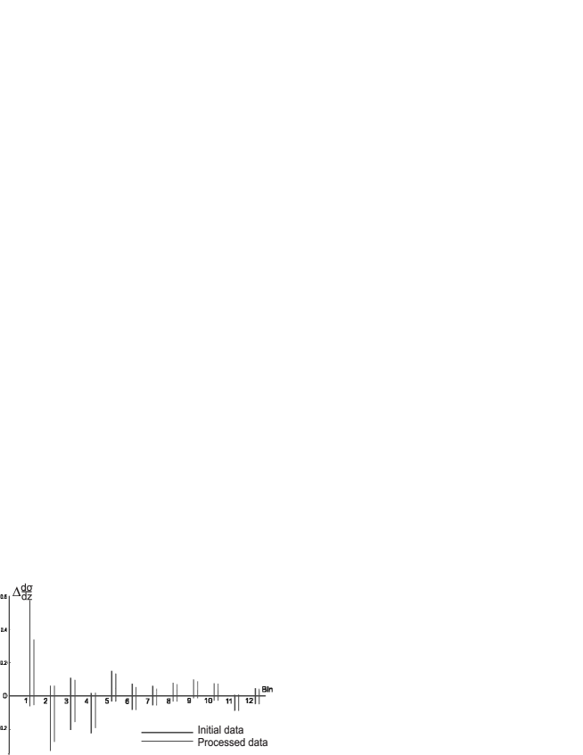
An overall distribution of the data is shown in Fig.1. As it is seen, this forms the set of segments determining the value of the cross-section with its uncertainty. To obtain a more strict constraint on the axial-vector $\bar{a}^{2}$ and vector $\bar{v}^{2}$ couplings squared, we have to decrease the lengths of segments. For this purpose the NN analysis is applied.

At first stage, the NNs were trained to recognize the signal and the background.

The contribution of the $Z^{\prime}$ to a differential cross-section for the Bhabha process obtained within the SM extended by $Z^{\prime}$ was taken as the signal. Analytic expression for this contribution reads [1]:

$$\frac{d\sigma^{Z^{\prime}}}{dz}=F_{v}(\sqrt{s},z)\bar{v}^{2}+F_{a}(\sqrt{s},z)\bar{a}^{2}+F_{av}(\sqrt{s},z)\bar{a}\bar{v}$$ (2)

where $F_{a}$ , $F_{v},F_{av}$ are the functions depend on the SM couplings. In actual analysis they have been calculated with accounting for the relations due to renormalizability. This contribution was computed for the values of $0.0\leq\bar{v}^{2}\leq 4\times 10^{-4}$ and $0.0\leq\bar{a}^{2}\leq 4\times 10^{-4}$. Such the choice is based on the results, obtained in [1].

As the background we set the deviation from the signal equaled to the redoubled uncertainty of LEP2 experimental data. Thus, the network was trained to discard data, which correspond to large deviations from the signal, but include the ones corresponding to the probable signal of the $Z^{\prime}$.

The NN processing makes the cutoff of the data. The cutoff eliminates the data which are assumed to be the background signal. Side by side with the background signals the NN could discard the signal data too. But total amount of these events is negligibly small as compared to the amount of discarded background points.

To create and train NNs the MLPFit program [6] was used. Three-layer NNs were used, with 2 neurons in input, 10 neurons in hidden and 1 neuron in output layer.

An input vector for the networks consists of the scattering sector and the differential cross-section for this sector. The training algorithm with back propagation of errors was used. The type of training - with tutor - was applied. We also worked out a necessary computer program to solve the problem.

During processing, the NNs discarded all the data that have produced a less than 0.9 at NN output. After NN processing, the length of segments was decreased. The total decrease of them is 3-27 percent (these values vary for different data sets). The comparative general plot of data set before and after the application of the NN is shown in Fig.2.

Figure 2: Plot of $e^{+}e^{-}\to e^{+}e^{-}$ process data before and after NN processing.

After NNs processing, the data were analyzed by means of the $\chi^{2}$ method. Denoting an observable by $\sigma_{i}$, one can construct the $\chi^{2}$-function

$$\chi^{2}(\bar{a},\bar{v}_{e})=\sum\limits_{i}[\frac{\Delta\sigma_{i}^{exp}-\Delta\sigma_{i}^{th}(\bar{a},\bar{v}_{e})}{\delta\sigma_{i}}]^{2},$$ (3)

where $\Delta\sigma^{exp}$ and $\delta\sigma$ is the deviation of the measured cross-section from the SM one and the uncertainty for the Bhabha process, and $\Delta\sigma^{th}$ is the calculated $Z^{\prime}$ contribution. The sum in Eq.(3) refers to either the data in one specific process or the combined data for several processes. By minimizing the $\chi^{2}$-function, the maximal-likelihood estimate for the $Z^{\prime}$ couplings was derived. The confidence area in the parameter space $(\bar{v},\bar{a})$ corresponding to the probability $\beta$ is defined as

$$\chi^{2}\leq\chi^{2}_{min}+\chi^{2}_{CL,\beta}$$ (4)

where $\chi^{2}_{CL,\beta}$ is the $\beta$-level of the $\chi^{2}$-distribution with 2 degrees of freedom.

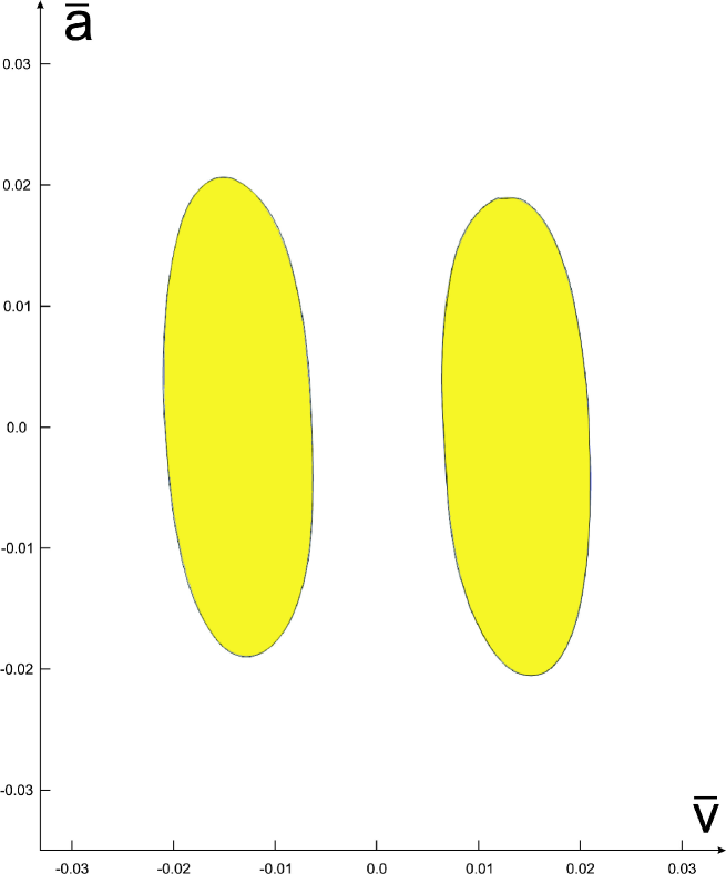
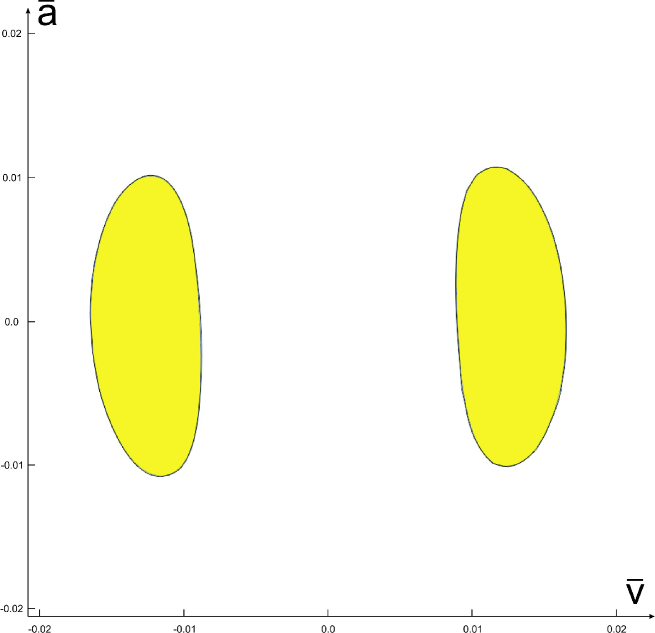
The analysis of the $\chi^{2}$-function for the $\bar{v}^{2}$ observable gives $\chi^{2}_{min}=158.49$ at $\bar{v}^{2}=2.37\times 10^{-4}$. The 95% CL area ($\chi^{2}_{CL}=5.99$) is shown in Fig.3. From this area the value $\bar{v}^{2}=(2.4\pm 1.99)\times 10^{-4}$ is obtained. The 95% CL area for data before the NN processing is shown in Fig.4.

Figure 3: The 95% CL in $\bar{v}-\bar{a}$ plane for $\bar{v}^{2}$ observable. The data set after the NN processing.

Figure 4: The 95% CL in $\bar{v}-\bar{a}$ plane for $\bar{v}^{2}$ observable. The data set before the NN processing.

The analysis of the $\chi^{2}$-function for the $\bar{a}^{2}$ observable results in $\chi^{2}_{min}=629.66$ at $\bar{a}^{2}=1.6\times 10^{-7}$. The 95% CL area ($\chi^{2}_{CL}=5.99$) is shown in Fig.5. To compare the results, the 95% CL area for data before NN processing is shown in Fig.6. As one can see, the zero point of $\bar{a}$ is inside the confidence area. So, we are able to obtain only an upper limit on its value $\bar{a}^{2}\leq 1.1\times 10^{-4}$ at the $2\sigma$ CL.

Figure 5: The 95% CL in $\bar{v}-\bar{a}$ plane for $\bar{a}^{2}$ observable. The data set after the NN processing. As it is seen, the zero point of $\bar{a}$ is inside the confidence area.

Figure 6: The 95% CL in $\bar{v}-\bar{a}$ plane for $\bar{a}^{2}$ observable. The data set before the NN processing.

To constrain the value of $Z^{\prime}$ mass by the derived bounds on the four-fermion couplings $\bar{v}^{2}$ let us assume that the coupling $\bar{g}$ is of the order of the SM gauge couplings, $\bar{g}^{2}/(4\pi)\simeq 0.01-0.03$. Then the obtained value $\bar{v}^{2}$ corresponds to $m_{Z^{\prime}}=0.53-1.05$ TeV.

In Ref. [1] the value $\bar{v}^{2}=2.18\pm 1.82\times 10^{-4}$ was obtained for the Bhabha process at the $2\sigma$ CL within one-parameter fit.

Table 1: Constraints on the $Z^{\prime}$ four-fermion couplings $\bar{v}^{2}$ obtained in different investigations

one-parameter fit		two-parameter fit	NN two-parameter fit
$1\sigma$	$2\sigma$	$2\sigma$	$2\sigma$
$\times 10^{-4}$
$2.24\pm 0.92$	$2.18\pm 1.82$	$\leq 1.44$	$2.4\pm 1.99$

3 Discussion

It is shown in Fig.2 how the NN selects data corresponding to the background. We note once again that the NN discards not only a background but also the signal. Nevertheless, the discarded signal data are negligibly small as compared to the discarded background ones.

The obtained values of $\bar{v}^{2}=(2.4\pm 1.99)\times 10^{-4}$ and $\bar{a}^{2}\leq 1.1\times 10^{-4}$ are comparable to the results obtained in [1]. In this paper the results were obtained within the one-parameter fit. In paper [2] it was shown that there is only a $1\sigma$ CL hint in the two-parameter fit. The analysis carried out in the present investigation shows the $2\sigma$ CL hint of the $Z^{\prime}$. The estimate of the mass value gives $m_{Z^{\prime}}=0.53-1.05$ TeV. This is signaling a comparably not heavy $Z^{\prime}$, that is of interest for the experiments at the Tevatron and LHC. The estimated couplings are also important to analyze the current and future experimental data.

To conclude, we note that the derived predictions of the NNs analysis of the two parameter fits are in good agreement with other one-parameter model-independent fits accounting for the $Z^{\prime}$ gauge boson existence [5], [2].

References

- [1] A.V. Gulov and V.V. Skalozub, Phys. Rev. D 70, 115010 (2004).
- [2] A.V. Gulov and V.V. Skalozub, Phys. Rev. D 76, 075008 (2007).
- [3] A. Leike, Phys. Rep. 317, 143 (1999).
- [4] T. G. Rizzo, Presented at 34th International Conference on High Energy Physics (ICHEP 2008), Philadelphia, Pennsylvania, 30 Jul - 5 Aug 2008.
- [5] A. Ferroglia, A. Lorca, J.J. van der Bij, Annalen Phys.16:563-578,2007
- [6] MLPFit, http://home.cern.ch/ schwind/MLPfit.html
- [7] V.M.Abazov et al. [D0 Collaboration], Phys. Lett. B 517, 282 (2001).
- [8] ALEPH Collaboration (R. Barate et al.), Eur. Phys. J. C 12, 183-207(2000); DELPHI Collaboration (J. Abdallah et al.), Eur. Phys. J. C 45, 589-632(2006); L3 Collaboration (M. Acciarri et al.), Phys. Lett. B 479, 101-117(2000); OPAL Collaboration (K. Ackerstaff et al.), Eur. Phys. J. C 2, 441-472(1998); OPAL Collaboration (G. Abbiendi et al.), Eur. Phys. J. C 6, 1-18(1999); OPAL Collaboration (G. Abbiendi et al.), Eur. Phys. J. C 33, 173-212(2004).
- [9] ALEPH Collaboration, DELPHI Collaboration, L3 Collaboration, OPAL Collaboration, the LEP Electroweak Working Group, the SLD Heavy Flavour, Electroweak Working Group, hep-ex/0511027.