A plastic flow theory for amorphous materials

Abstract

Starting from known kinematic picture for plasticity, we derive a set of dynamical equations describing plastic flow in a Lagrangian formulation. Our derivation is a natural and a straightforward extension of simple fluids, elastic and viscous solids theories. These equations contain the Maxwell model as a special limit. We discuss some results of plasticity which can be described by this set of equations. We exploit the model equations for the simple examples: straining of a slab and a rod. We find that necking manifests always itself (not as a result of instability), except if the very special constant-velocity stretching process is imposed.

Plastic materials exhibit several features which are not present in the usual liquids or solids. Their dynamics consist in a nontrivial mixture of liquid-like and solid-like behaviors. Understanding plasticity in metal industry and, in general, in technology, is of a paramount importance. Nonetheless, to date no universal dynamical equations describing plastic materials like Navier-Stokes equations for fluids, and Lamé equations for elastic solids, are available. Under strain, plastic material may exhibit elastic-like behaviors, yield stress, flowing behaviors, nonlinear engineering strain-stress relation, and so on Malverne . A major goal in material science is the description of these phenomena in terms of dynamical evolution equations for relevant variables, namely the velocity, stress, and the analogues of strain.

There has been important contributions to the theory of plasticity, especially for crystalline materials in terms of dislocations LL7 ; Kubin ; Groma . However, there is no need to evoke dislocations (if ever this notion has a meaning) for amorphous materials, and thus the question arises of how a corresponding theory can be build at the continuum level. This question has known recently an upsurge of interest ELP . An essential issue when addressing the question of plasticity is the distinction between crystalline solids and amorphous materials. Elastically deformed monocrystals are in a metastable state. Their plastic flow takes place only upon creation of dislocations, and is thus a nonlinear process. Conversely, plastic flow of amorphous materials should occur, in principle, linearly with respect to the applied stress. In crystals, an additional field, namely dislocation density, is introduced which couples to the elastic as well as to plastic distorsions Kubin ; Groma . It is proposed here that one can derive a plastic continuum theory for amorphous materials, without evoking neither dislocation density, nor an internal variable that is distinct from the variables describing usual kinematics of plasticity. The evolution equations can be written in a closed form in terms of the elastic and plastic distorsions only. The concept of distortion LL7 used here was introduced by Kröener and Rieder in 1956 Kroner , and will constitute our basic definition of the plastic flow variable.

If $u_{k}$ denotes the $k^{th}$ component of the displacement field, then the total distorsion tensor reads $\partial_{i}u_{k}$. For a purely elastic solid, and in the small deformation regime, the symmetrized part ${u_{ik}=(\partial_{i}u_{k}+\partial_{k}u_{i})/2}$ is the strain tensor. If plastic flow is involved, the total distorsion tensor $\partial_{i}u_{k}$ is a sum of the plastic flow contribution $w^{pl}_{ik},$ and the elastic part $w_{ik}$ (see LL7 )

$$\partial_{i}u_{k}=w^{pl}_{ik}+w_{ik}.$$ (1)

The symmetrical part of the elastic distortion defines the strain tensor

$$u_{ik}=\frac{1}{2}(w_{ik}+w_{ki}).$$ (2)

The constrain ${w^{pl}_{ii}=0}$ is usually supposed. Then from Eqs.(1,2) it follows ${u_{ii}=\partial_{i}u_{i}.}$

Usual elasticity can be presented in a Lagrangian manner by introducing an energy and a dissipative function. The elastic energy of a solid is given by

$$\frac{\lambda}{2}u^{2}_{ll}+\mu u^{2}_{ik},$$ (3)

here $\lambda,\mu$ are Lamé coefficients, and the kinetic energy is $\rho{\bf v}^{2}/2,$ where $\rho$ is the density of the material. The dissipation function reads for a viscous solid

$$\eta^{s}\left(\dot{u}_{ik}-\frac{1}{3}\delta_{ik}\dot{u}_{ll}\right)^{2}+\frac{\zeta}{2}\dot{u}_{ll}^{2}$$ (4)

In the presence of a plastic flow one must introduce a new additional dissipative part related to plasticity. The system is described by three independent tensors, namely $u_{ik}$, and $w^{pl\pm}_{ik}$ which are the symmetric $(+),$ and antisymmetric $(-)$ parts of the plastic distortion tensor, respectively. From the basic kinematic relation (1) and the strain tensor definition (2) it follows

$$w^{pl+}_{ik}=\frac{1}{2}(\partial_{i}u_{k}+\partial_{k}u_{i})-u_{ik}.$$ (5)

We expect the dissipation to consist of a quadratic form of these quantities, that we write as

$$2\alpha\dot{u}_{ik}\dot{w}^{pl+}_{ik}+\eta\left(\dot{w}^{pl+}_{ik}\right)^{2}+\gamma\left(\dot{w}^{pl-}_{ik}\right)^{2}$$ (6)

This is the dissipation corresponding to plastic flow. Stability criteria for the dissipation function enforce ${\eta^{s}>0,}$ ${\zeta>0,}$ ${\eta\eta^{s}>\alpha^{2},}$ ${\gamma>0.}$ Note that there is only one dilatational viscosity constant $\zeta.$ All other constants are related with shear motions. As we will see below in the liquid limit the constant $\eta$ is a usual hydrodynamic viscosity.

The strategy now consists in performing variations of the total Lagrangian with respect to the independent variables. Variation with respect to $\delta{\bf u},$ with ${\delta w^{pl}_{ik}=0},$ yields, upon using, ${2\delta u_{ik}=\partial_{i}\delta u_{k}+\partial_{k}\delta u_{i},}$ the momentum conservation law

$$\rho\ddot{u}_{i}=\partial_{k}\sigma_{ik}$$ (7)

with the stress tensor $\sigma_{ik}$ consisting of a sum of the usual elastic part as well as the dissipative part with the usual solid viscosity terms, and an additional plastic term

$$\sigma_{ik}=\lambda u_{ll}\delta_{ik}+2\mu u_{ik}+$$

$$+2\eta^{s}\dot{u}_{ik}+\left(\zeta-\frac{2}{3}\eta^{s}\right)\delta_{ik}\dot{u}_{ll}+2\alpha\dot{w}^{pl+}_{ik}.$$ (8)

Variation with respect to ${\delta w^{pl+}_{ik}},$ with ${\delta{\bf u}=0},$ and ${\delta w^{pl-}_{ik}=0}$ (in that case ${\delta u_{ik}=-\delta w^{pl+}_{ik}}$) provides us with

$$\tilde{\sigma}_{ik}=\alpha\left(2\dot{u}_{ik}-\frac{2}{3}\delta_{ik}\dot{u}_{ll}\right)+2\eta\dot{w}^{pl+}_{ik},$$ (9)

here $\tilde{\sigma}_{ik}$ is the traceless part of $\sigma_{ik}$.

Finally, variation with respect to ${\delta w^{pl-}_{ik}},$ with ${\delta{\bf u}=0},$ and ${\delta w^{pl+}_{ik}=0}$ (in that case ${\delta u_{ik}=0}$) leads to ${\dot{w}^{pl-}_{ik}=0}$ (a direct consequence of the absence of dissipation for rigid rotation; note also that energy does not depend on that mode).

An important remark is in order. Differentiating (1) with respect to time one obtains

$$\partial_{k}v_{i}+\partial_{k}v_{i}=-2j_{ik}^{pl}+2\dot{u}_{ik}$$ (10)

where ${j_{ik}^{pl}\equiv-{\dot{w}^{pl+}_{ik}},}$ is the plastic current. This equation (see also LL7 ), apart from the (conventional) minus sign in front of $j_{ik}^{pl},$ bears resemblance with Eq.(3) of Ref. ELP . There is, however, a fundamental difference. Indeed, Eq.(3) of Ref. ELP uses the kinematic condition (10), plus Hooke’s law, where $u_{ik}$ is assumed to be related to the stress tensor by

$$u_{ik}={\tilde{\sigma}_{ik}\over 2\mu}-{p\over 2K},$$

where ${p=-\sigma_{kk}/2},$ is the pressure, and $K$ and $\mu$ are the compressibility and the shear modulus (note that a 2D geometry is assumed in Ref. ELP ). In the present study we do not postulate a priori a Hooke’s relation, since both elastic and plastic contributions are embedded together within the total distortion tensor $\partial_{i}u_{k}.$ The relation between $u_{ik}$ and $\sigma_{ik}$ follows here as a consequence of the Lagrangian formulation, and the relationship between these two quantities is provided by (8) (showing that a measure of the stress is a combination of elastic and plastic deformations).

It is possible to express the plastic distortion tensor in terms of other quantities. From Eqs.(8-9) we may express $\sigma_{ik}$ in terms $u_{ik}$ and its time derivative. It is convenient to split the stress tensor $\sigma_{ik}$ into a traceless and a pressure-like term (actually the trace of $\sigma_{ik}$):

$$\sigma_{ik}=\frac{1}{3}\delta_{ik}\sigma_{ll}+\tilde{\sigma}_{ik}$$ (11)

The trace has a usual elastic (including the dissipative part) form

$$\sigma_{ll}=(3\lambda+2\mu)u_{ll}+3\zeta\dot{u}_{ll}.$$ (12)

The traceless parts of the stress tensor are connected with each other and with spatial gradients of the velocity by the following two relations

$$(\eta-\alpha)\tilde{\sigma}_{ik}=2\eta\mu\tilde{u}_{ik}+2(\eta\eta^{s}-\alpha^{2})\dot{\tilde{u}}_{ik},$$ (13)

$$\tilde{\sigma}_{ik}+2(\eta-\alpha)\dot{\tilde{u}}_{ik}=\eta\left(\partial_{i}v_{k}+\partial_{k}v_{i}-\frac{2\delta_{ik}}{3}\partial_{l}v_{l}\right).$$ (14)

The first relation is obtained by expressing $\dot{\omega}^{pl}_{ik}$ from Eq. (9) and inserting the resulting relation into (8). The second one follows from Eq. (9) by using relation (5). The set of Eqs. (7,11-14) defines space-time evolution of displacement vector ${\bf u},$ strain $u_{ik}$ and the stress tensor $\sigma_{ik}$. This constitutes a complete set of equations for the three (vectorial and tensorial ) quantities ${\bf u},$ $u_{ik}$ and $\sigma_{ik}$ (we could, of course, alternatively use other quantities like $w_{ik}^{pl+}$). Note that Eq. (14) has some similarity with the Maxwell model, used to describe plasticity with a yield stress in some models saramito . There is an important difference, however. Instead of the $\dot{\sigma}_{ik}$ on the l.h.s. we have $\dot{u}_{ik}.$ Again this consistently follows from the Lagrangian formulation.

The Maxwell model of liquids with high viscosity can be obtained from our equations only if one consider the incompressible limit and set $\alpha=\eta^{s}=\zeta=0.$ This leads, from Eq. (13), to ${\sigma_{ik}=2\mu u_{ik}}.$ Eq. (14) reduces to the well known Maxwell form

$$\dot{\sigma}_{ik}+\mu\eta^{-1}\sigma_{ik}=\mu(\partial_{i}\dot{u}_{k}+\partial_{k}\dot{u}_{i}).$$ (15)

Let us present few examples where we could obtain an exact solution of the plastic dynamics. Consider an induced oscillatory motion in the material. We assume a semi-infinite medium bounded by a planar surface which undergoes oscillations in its own $xz-$plane: ${u_{x}(t,0)=u\cos\omega t.}$ In this case the nonzero components of the fields are $u_{x},$ $u_{xy},$ $w_{xy},$ $w_{yx},$ $w^{pl+}_{xy},$ and $\sigma_{xy}.$ Then the set of Eqs. (7,13,14) reads:

$$\rho\ddot{u}_{x}=\partial_{y}\sigma_{xy}=\partial_{y}\frac{2\eta\mu u_{xy}+2(\eta\eta^{s}-\alpha^{2})\dot{u}_{xy}}{\eta-\alpha};$$ (16)

$$\mu u_{xy}+(\eta-2\alpha+\eta^{s})\dot{u}_{xy}=\frac{\eta-\alpha}{2}\partial_{y}v_{x}.$$ (17)

It is then found that each field is a linear combination of the complex modes ${\propto\exp(-i\omega t+i\kappa y)},$ where $\kappa$ is defined by

$$\kappa^{2}=(\kappa^{\prime}+i\kappa^{\prime\prime})^{2}=i\frac{\omega\rho}{\eta}\left(1-\frac{i\omega(\eta-\alpha)^{2}}{\eta\mu-i\omega(\eta\eta^{s}-\alpha^{2})}\right).$$ (18)

For example, the displacement field is ${u_{x}=u\cos(\omega t-\kappa^{\prime}y)\exp(-\kappa^{\prime\prime}y).}$ The low frequency limit recovers a known Stokes result for a shear viscous mode in liquids (see §24 in LL6 ). Elastic solid behavior (an emission of shear sound) corresponds to the limit of high plastic viscosity ${\eta\rightarrow\infty}.$

We would like to point out some results that can be captured analytically in some special limit. The long time behavior of a slab under tension, is expected to be dominated by plastic flow. Ultimately, the plastic flow should look-like a hydrodynamical flow. Let us concentrate on this limit. Consider a plate (or a rod) of a plastic material with free surfaces (Fig. 1). This is a similar geometry to that treated in Ref. ELP . The plate is stretched along the $x$ direction. For a flat geometry we have obtained an exact solution with the plate thickness $h(t)$ that depends only on the $t$ variable. This type of solution exists only in the case where the stretching occurs at a given constant velocity. Let us first motivate the solution on the basis of symmetries. Because of the axial symmetry with respect to the $y$ axis at ${x=0},$ $v_{x}$ must be zero on that line. For constant $h$ there is a simple solution that fulfills that symmetry, ${v_{x}=cx},$ where $c(t)$ is for the moment an arbitrary function of time. From incompressibility condition we have ${v_{y}=-cy+g(x,t),}$ where $g$ is a priori an arbitrary function of $x$ and $t.$ Symmetry with respect the middle line ${y=0},$ enforces ${g=0}.$

We straightforwardly obtain from the Navier-Stokes equation the pressure field

$$p=-\rho(\dot{c}+c^{2})\frac{x^{2}}{2}+\rho(\dot{c}-c^{2})\frac{y^{2}}{2}+f(t),$$

where $f(t)$ is a function of time to be determined below. At the free surface the normal component of the stress (the tangential vanishes automatically) must vanish. This is easily computed from the above result by using the definition ${\sigma_{yy}=-p+2\eta\partial_{y}v_{y}=-p-2\eta c.}$ Imposing ${\sigma_{yy}=0}$ on the free surfaces at ${y=\pm h,}$ at any $x,$ we obtain ${\dot{c}+c^{2}=0.}$ This provides us with ${c=(t-t_{0})^{-1}},$ where $t_{0}$ is a constant of integration. It is convenient to measure the time from the moment $t_{0},$ so we will set ${t_{0}=0}.$

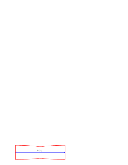
Figure 1: A sketch of the geometry under consideration.

For the length of the strip $L,$ one has ${\dot{L}=cL,}$ so that ${L=st,}$ with constant velocity $s.$ Due to mass conservation one obtains that ${h=\gamma/t,}$ where the total volume is defined as $\gamma s.$ The solution corresponds to stretching plastic flow for ${t>0}$, and ${s,\gamma>0,}$ while for ${t<0},$ and ${s,\gamma<0,}$ it represents a contracting flow.

Reporting this solution into the above-mentioned boundary conditions fixes the function ${f(t)=\rho\gamma^{2}t^{-4}-2\eta t^{-1}}.$ The $xx$-component of the stress tensor is ${\sigma_{xx}=-p+2\eta\partial_{x}v_{x}=-p+2\eta c.}$ The total force of stretching is defined as

$$F_{2d}\equiv\int_{-h}^{h}dy\sigma_{xx}=-{4\over 3}\rho{\gamma^{2}h\over t^{4}}+{8\eta h\over t}.$$ (19)

The first part is inertial, while the second one is viscous. The viscous part dominates at long time such that ${t\gg\gamma^{2/3}\nu^{-1/3},}$ where ${\nu=\eta/\rho}$ is the kinematic viscosity.

It is a simple matter to extend the calculation to a cylindrical geometry (stretching of a rod) following precisely the same line. We only give the results: The velocity is given by ${v_{z}=cz},$ ${v_{r}=-cr/2},$ with ${c(t)=t^{-1}}$. The pressure reads

$$p=\frac{3\rho}{8t^{2}}\left(\frac{\gamma^{2}}{t}-r^{2}\right)-\frac{\eta}{t}.$$

We obtain for the length and the radius ${L=st},$ ${a=\gamma/\sqrt{t}.}$ The volume is given by ${\pi a^{2}L=\pi s\gamma^{2}}.$ The total axial force in the rod stretching problem is

$$F_{3d}\equiv 2\pi\int_{0}^{a}rdr\sigma_{zz}=-\frac{3}{16}\frac{\rho\gamma^{2}}{t^{3}}S+3\frac{\eta}{t}S,$$ (20)

where ${S=\pi a^{2}}$ is a rod cross section area.

The above solutions exists only for a constant velocity stretching. The question thus naturally arises of what happens if an other process is imposed. This is what we would like to investigate now. Following Ref.ELP , if the lateral boundary of the plate moves at a pre-determined strain rate $\dot{L}/L=\Omega=const.,$ then our result shows that a homogeneous thinning of the strip is not possible. Thus a modulated strip prevails. This is a precursor of the necking problem. Thus necking appears here as natural phenomenon due to material flowing Hutchinson whenever the stretching is not performed at a constant speed. The necking is not related with an instability ELP , but rather the fact that a homogeneous thinning does not exist (except if ${L(t)\propto t}$) in plastic dynamics.

Let us investigate the stability of the homogeneous solutions. We consider deviations with large wavelengths as compared with the layer thickness. By analogy with the theory of shallow water (see LL6 §108) we derive effective hydrodynamic equations in terms of the thickness $h,$ and velocity $v$ along $x$. Mass conservation yields

$$\dot{h}+\partial_{x}(hv)=0.$$ (21)

Note, that when the viscous term dominates, one can rewrite the total force (19) as follows ${F_{2d}=-8\eta\partial_{t}h}.$ In a general case of inhomogeneous shape one should have ${F_{2d}=-8\eta(\dot{h}+v\partial_{x}h)}.$ Consequently the momentum conservation law in this purely viscous limit has the form

$$h(\dot{v}+v\partial_{x}v)=-8\nu\partial_{x}(\dot{h}+v\partial_{x}h).$$ (22)

From Eqs.(21,22) one obtains upon linearization about the 2D homogeneous solution: ${t\delta\dot{h}+x\partial_{x}\delta h+\gamma\partial_{x}\delta v+\delta h=0}$, and ${\gamma(t\delta\dot{v}+x\partial_{x}\delta v+\delta v)=-8\nu t\partial_{x}(t\delta\dot{h}+x\partial_{x}\delta{h}).}$ Introducing the new coordinate ${\tilde{x}=x/t}$ one arrives at: $t^{2}\delta\dot{h}+\gamma\delta v^{\prime}+t\delta h=0,$ and $\gamma(t\delta\dot{v}+\delta v)=-8\nu t\delta\dot{h}^{\prime}.$ Taking the Fourier transform ${\propto\exp(iq\tilde{x})},$ we find for a given mode with wavenumber $q$ of one of the fields, say $\delta h:$ ${t^{2}\delta\ddot{h}+4(t+\tau)\delta\dot{h}+2\delta h=0},$ here ${\tau=2\nu q^{2}.}$ This equation has a first integral ${t^{2}\delta\dot{h}+2t\delta h+4\tau\delta h=C,}$ where $C$ is a constant. One obtains finally

$$\delta h=\frac{C}{t^{2}}\exp\left(\frac{4\tau}{t}\right)\int^{t}_{t^{*}}\exp\left(-\frac{4\tau}{t}\right)dt,$$

where $t^{*}$ is a second constant of integration. At large time, ${t\gg\tau},$ the deviation amplitude is ${\delta h=Ct^{-1}\{1-4\tau t^{-1}\ln(t/et^{*})\}.}$ It decays mostly as $t^{-1}$ like the strip thickness $h.$ Consequently, one may say that the solution is marginally stable for large wavelength fluctuations.

The 3D problem of the rod stretching with small inhomogeneity can be formulated in the same manner (Eqs.(21,22)). The results are identical to the 2D ones, if one makes the substitutions ${h\rightarrow S},$ and ${8\nu\rightarrow 3\nu}.$

We have solved Eqs.(21)-(22) numerically in the fully nonlinear regime. We give here the major results: (i) If one imposes a constant stretching we find that the ultimate stage is a homogeneous thickness that decreases in time as $1/t,$ in agreement with our analytical results. (ii) Starting from a small perturbation (of sine type), we observe marginal stability. (iii) Most importantly, we have found that if the stretching velocity is not constant the ultimate stage is a modulated thickness, of necking type. In fact, Fig.1 represents the result of our numerical solution, that exhibits necking in the case of initially flat plate and ${\dot{L}/L=const.}$ (same stretching law as in Ref. ELP ). This behavior is found for various initial conditions, and (non constant) stretching laws. Thus necking seems to be a robust feature, which takes place whenever the stretching is non constant.

It should be mentioned that here our plastic equations have been written by disregarding the so-called objective derivative (we have used ordinary derivatives) for tensors. One alterative in order to confer an objective form to these equations, is to replace the time derivative of tensors by the so-called co-rotational derivativeBird1 , as is done in ELP . We shall report on full numerics of our completed set of equations (7,11-14) in the future.

We acknowledge CNRS, Univ. J. Fourier, and CNES for financial support.

References

- (1) L.E. Malverne, Introduction to the Mechanics of a Continuous Medium (Prentice Hall, INc. New Jersey, 1969); J. Lubliner, Plasticty Theory (Macmillan Publishing Compagny, New York, 1990); Unified Constitutive Laws of Plastic Deformation, edited by A.S. Krausz and K. Krausz (Academic Press, San Diego, 1996).
- (2) L.D. Landau and E.M. Lifshitz, Theory of Elasticity, Pergamon Press, Oxford (1987).
- (3) V. Bulatov, F. Abraham, L. Kubin, Devincre, and S. Yip, Nature 391, 669 (1998), and references therein.
- (4) I. Groma and B. Bakò, Phys. Rev. Lett. 84, 1487 (2000).
- (5) L.O. Eastgate, J.S. Langer, and L. Pechelnik, Phys. Rev. Lett. 90, 045506 (2003), and references therein.
- (6) E. Kröener and R. Rieder, Z. Phys. 145, 424 (1956).
- (7) P. Saramito, J. Non-Newtonian Fluid Mech. 145, 1 (2007), and refernces therein.
- (8) L.D. Landau and E.M. Lifshitz, Fluid Mechanics, Butterworth-Heinemann, Oxford (2000).
- (9) J.W. Hutchinson and K.W. Neale, Acta Metall. 25, 839 (1977).
- (10) R. B. Bird, R. C. Armstrong, and O. Hassager, Dynamics of Polymeric Liquids, Vol. 1, Fluid Dynamics,” Wiley, New York (1977, 2nd edition 1987).