The visibility of low-frequency solar acoustic modes

Abstract

We make predictions of the detectability of low-frequency p modes. Estimates of the powers and damping times of these low-frequency modes are found by extrapolating the observed powers and widths of higher-frequency modes with large observed signal-to-noise ratios. The extrapolations predict that the low-frequency modes will have small signal-to-noise ratios and narrow widths in a frequency-power spectrum. Monte Carlo simulations were then performed where timeseries containing mode signals and normally distributed Gaussian noise were produced. The mode signals were simulated to have the powers and damping times predicted by the extrapolations. Various statistical tests were then performed on the frequency-amplitude spectra formed from these timeseries to investigate the fraction of spectra in which the modes could be detected. The results of these simulations were then compared to the number of p-modes candidates observed in real Sun-as-a-star data at low frequencies. The fraction of simulated spectra in which modes were detected decreases rapidly as the frequency of modes decreases and so the fraction of simulations in which the low-frequency modes were detected was very small. However, increasing the signal-to-noise (S/N) ratio of the low-frequency modes by a factor of 2 above the extrapolated values led to significantly more detections. Therefore efforts should continue to further improve the quality of solar data that is currently available.

1 Introduction

To date a multitude of solar acoustic (p) modes have been observed over a wide range of frequencies. However, no independently confirmed detections of low-degree (low-$l$) p modes, with frequencies below $\sim 970\,\rm\mu$Hz, have been made (e.g. [García et al. 2001]; [Chaplin et al. 2002]; [Broomhall et al. 2007]). As low-frequency p modes are expected to have very long lifetimes their detection would allow their frequencies to be measured to very high accuracies and precisions. This is crucially important as the properties of low-$l$ p modes are affected by conditions deep in the solar interior and so their frequencies act as a probe of these regions. However, the signal from low-frequency p modes is very weak. Therefore, different analysis procedures have been developed in attempts to detect these modes.

Broomhall et al. (2007) used statistical techniques to look for coincident prominent features in BiSON and GOLF frequency-amplitude spectra. They found that many low-frequency p modes remain undetected despite reducing amplitude detection thresholds to less than $3$ mm s^-1 bin^-1/2. However, Broomhall et al. found the $l=0$, $n=6$ mode at $\sim 973\,\rm\mu Hz$ to be extremely prominent. This mode has also been detected in other studies such as Garcia et al. (2001) and Chaplin et al. (2002). The prominence of this mode is conspicuous because of the lack of evidence for higher-frequency modes such as the $l=0$, $n=7$ mode at $\sim 1118\,\rm\mu Hz$. As yet this mode has only been observed in Sun-as-a-star data by Garcia et al. (2001). These higher-frequency modes should be easier to observe as theoretically they should exhibit larger amplitudes in the photosphere, where the observations are made. It is, therefore, of interest to investigate how prominent the $l=0$, $n=6$ mode, and the modes surrounding it in frequency, should be. This will provide an indication as to whether we should be observing modes that we are not; or whether some effect makes the $l=0$, $n=6$ mode more prominent than the rest.

How easy low-frequency modes are to detect depends upon their power and width in a frequency-power spectrum. As many low-frequency modes have not yet been detected their powers cannot be determined from solar data directly. Here, predictions of the power in very low-frequency modes have been made by extrapolating the power observed in well-defined, higher-frequency modes. The height of a mode in a frequency spectrum also depends upon the width in frequency over which the power is spread. As the power in the signal from a mode is damped over time the signal from the mode may be spread over several bins of a frequency spectrum. The lifetime of a mode varies with frequency and so it is also possible to infer from extrapolation the width a mode at a particular frequency is expected to exhibit from results for well-observed modes. The details of how the extrapolations were made will be explained in Section 2. To make the extrapolations we have assumed that the simple functional relationships that turn out to describe the powers and heights of the well-observed modes are still valid at low frequencies. The validity of this assumption was tested using predictions of the powers and widths of low-frequency modes made by the Cambridge stochastic excitation and damping codes (e.g. Houdek et al. 1999). Monte Carlo simulations based on the results of the extrapolations were then performed to investigate how often simulated modes could be detected (Section 3). The simulations involved creating timeseries to mimic Sun-as-a-star data. The simulated data contained mode signals that have the properties predicted by the extrapolations. Various statistical tests, which are described in Section 4, were performed on the frequency-amplitude spectra that were created from the simulated timeseries. The statistical tests followed those described in Broomhall et al. (2007) and determined how often the simulated modes could be detected. The results of these tests are detailed in Section 5. A discussion of the results is presented in Section 6. In this discussion we pay particular attention to the unusual $l=0$, $n=6$ radial mode.

2 Predicting the Widths and Powers of modes

Various properties of modes can be found by fitting frequency-power spectra. These properties include the width of a mode, and therefore its damping time, and the height of a mode, i.e. its maximum power spectral density. The product of the height and width is proportional to the total power in the mode. A BiSON spectrum, consisting of 3071 d of Sun-as-a-star Doppler velocity observations, was fitted using the methods described in [Fletcher (2007)]. The fitting procedure involved taking the Fourier transform of the timeseries to produce a frequency-power spectrum and then fitting a Lorentzian-like model to the various mode peaks in the resulting frequency-power spectrum. The observations were made between 1996 April 20 and 2004 September 15, an epoch which spans most of solar activity cycle 23. The data were processed in the manner described by [Appourchaux et al. (2000)] and Chaplin et al. (2002). The data were the same as the BiSON data used in Broomhall et al. (2007) except that, instead of being rebinned to have a cadence of $120\,\rm s$, the data were left with the nominal $40\,\rm s$ cadence on which the BiSON data are stored.

The visibility of a mode in a frequency-power spectrum will depend on the power and lifetime of the mode. We will now briefly discuss how these properties affect the visibility.

2.1 How the power and width of a mode affects its visibility

The width of a mode, $\Delta$, is related to its lifetime, $\tau$, by

$$\Delta=\frac{1}{\pi\tau}.$$ (1)

If the length of a timeseries is significantly longer than the lifetime of a mode the timeseries will extend over several realizations of the mode and so the modal peak will be resolved across several bins in the frequency domain. However, if a mode’s lifetime is significantly longer than the length of a timeseries all of the mode’s power will be contained in a single bin.

If the width of a mode can be resolved the power of that mode, $V^{2}$, is given by

$$V^{2}=\frac{\pi}{2}T\Delta H,$$ (2)

where $T$ is the length of the timeseries and $H$ is the maximum power spectral density per bin. When the power spectrum is fitted it is actually the maximum power spectral density, which corresponds to the height, $H$, of the Lorentzian, that is determined. The width, $\Delta$, and height, $H$, of the mode can then be used to find the power of the mode. In this paper the observed signal-to-noise ratio of a mode refers to the ratio of the height of the most prominent spike across the width of the mode and the mean level of the background around it. We define a spike as the power (or amplitude) contained in one bin in a frequency-power (or amplitude) spectrum. The height of the most prominent spike of a resonant peak in a frequency-power spectrum will be greater than the height of the fitted Lorentzian. This is because of the random nature of the excitation of the modes, which means that the power will have a $\chi^{2}$ 2 degrees of freedom distribution about the underlying Lorentzian. Therefore, the power in some of the bins across the width of the mode will be greater than the height of the Lorentzian. These are the spikes that are most likely to be detected.

Notice that it is the power, $V^{2}$, that we are going to extrapolate and not the peak height of the mode. This is because the height, $H$, of the mode is not a smooth function of frequency, as it depends on whether the power of the mode is spread over more than one bin or whether the mode’s power is confined to one bin only. On the other hand the power of a mode is a smooth function of frequency and so can be extrapolated more easily.

A well-defined mode is one with a power and a width that are sufficiently large for the mode to be detected easily, allowing the shape of the mode in a frequency-power spectrum to be fitted accurately. In the case of the Sun, when fitting a set of data that spans $\sim 8.5\,\rm yr$, well-defined modes have frequencies greater than $\sim 1500\,\rm\mu Hz$. Here we are concerned with modes at low frequencies that cannot be observed clearly. Therefore it was necessary to extrapolate the widths and powers of well-defined modes to obtain estimates of the widths and powers of low-frequency modes. We have, therefore, assumed that simple functional relationships, which describe the variation of the parameters with frequency at higher frequencies, persist to lower frequencies. In section 2.5 we have used predictions from a stochastic excitation model to test the validity of this assumption. The extrapolation can be performed in two different ways, each of which will now be described in turn.

2.2 Method 1: The ln-linear relationship

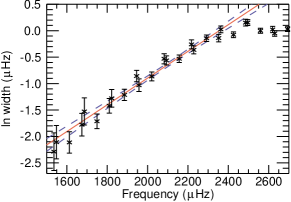
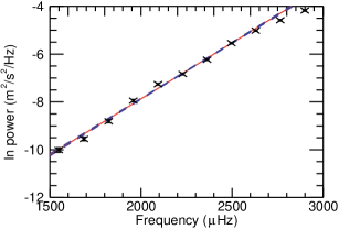
Figure 1: Results for method 1. Top panel: The black crosses show how the natural logarithm of the observed width of a mode varies with frequency. The widths have been plotted for modes with $l=0$, 1 and 2. The errors of the widths are those associated with the fits. The red solid line shows the linear line of best fit for the widths at frequencies between $\sim 1530\,\rm\mu Hz$ and $\sim 2400\,\rm\mu Hz$. The blue dashed lines indicate the errors on this linear fit. Bottom panel: The black crosses show how the natural logarithm of a mode’s power varies with frequency. The powers have been plotted for $l=0$ modes only. The red solid line shows the linear line of best fit for the powers at frequencies between $\sim 1540\,\rm\mu Hz$ and $\sim 2500\,\rm\mu Hz$. The blue dashed lines indicate the errors on this fit.

For well-defined modes with frequencies below $\sim 2400\,\rm\mu Hz$ an approximately linear relationship is observed between the natural logarithm of a mode’s width and its frequency (see the top panel of Figure 1). The well-defined plateau in the mode widths above $\sim 2400\,\rm\mu Hz$ (see for example [Chaplin et al. 2005]) means that the linearity does not extend to higher frequencies. The observed widths have been fitted using data from modes with different degrees. In Sun-as-a-star observations only low-$l$ modes can be clearly observed. Here widths from $l=0$, 1 and 2 modes have been used. The width of a mode is not independent of degree as high-$l$ modes have a lower inertia than low-$l$ modes and so high-$l$ modes have faster damping rates. However, the difference in damping rates is minimal over the confined range of $l$ used here.

The relationship between the natural logarithm of a mode’s power and its frequency is also approximately linear for well-defined modes with frequencies below $\sim 2500\,\rm\mu Hz$ (see the bottom panel of Figure 1). The Doppler velocity variations that a mode exhibits over the solar disc are characterized by the spherical harmonics that describe the mode, and so are reliant on degree. The observed power is then dependent on the sensitivity of the observing instrument to the distribution of the line-of-sight velocities over the portion of the solar disc that is being observed. The bottom panel of Figure 1 shows the results for $l=0$ modes only. The power is calculated from equation 2 using the width and the height of the best fit Lorentzian for the mode. The width and height of a mode have a negative correlation of $\sim 0.95$ and so the resulting error bars on the calculated powers are small.

For both the power and the width a linear, least-squares fit was performed to determine the gradients and the zero-frequency intercepts. The gradients and zero-frequency intercepts of these fits and the errors associated with them can be seen in Table 1. This method of fitting the data will be referred to as method 1.

2.3 Method 2: The ln-ln relationship

An approximately linear relationship is also observed between the natural logarithm of the width of a mode and the natural logarithm of its frequency (see the top panel of Figure 2). Once again the linearity is only found at frequencies below $\sim 2400\,\rm\mu Hz$. Likewise an approximately linear relationship is found when the natural logarithm of the power of a mode is plotted against the natural logarithm of the frequency of that mode (see the bottom panel of Figure 2). As with method 1 a linear least squares fit was performed to find the gradients and the zero-frequency intercepts for both the width and the power. The gradients and zero-frequency intercepts resulting from fitting the powers and widths in this manner can be seen in Table 1. This approach to fitting the data will be referred to as method 2.

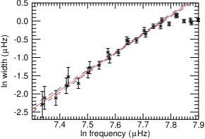
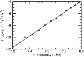
Figure 2: Results for method 2. Top panel: The black crosses show how the natural logarithm of the observed width of a mode varies with the natural logarithm of its frequency. The errors bars shown for the widths are those associated with the fits. The widths have been plotted for modes with $l=0$, 1 and 2. Bottom panel: The black crosses show how the natural logarithm of the mode power varies with the natural logarithm of mode frequency. The powers have been plotted for $l=0$ modes only. As in Figure 1 the red solid lines in both panels represent the linear best fits and the blue dashed lines represent the errors on the fits.

Table 1: Gradients and zero-frequency intercepts found by least squares fits for method 1 and method 2. The reduced $\chi_{\nu}^{2}$ value for each fit is also given.

	Gradient	Zero-frequency Intercept	$\chi_{\nu}^{2}$
Width
Method 1	$(2.5\pm 0.1)\times 10^{-3}$	$-6.0\pm 0.2$	0.91
Method 2	$(5.2\pm 0.2)\times 10^{0}$	$-40\pm 2$	0.70
Power
Method 1	$(4.68\pm 0.06)\times 10^{-3}$	$-17.2\pm 0.1$	6.5
Method 2	$(9.8\pm 0.1)\times 10^{0}$	$-82.3\pm 0.9$	6.9

2.4 Extrapolating method 1 and method 2 to low frequencies

To determine the value of the width and power of a mode at very low frequencies the gradients and zero-frequency intercepts were used to extrapolate the linear relationships from method 1 and method 2 to lower frequencies. The widths found using both method 1 and method 2 for $l=0$ modes, in the frequency range $800$ to $1450\,\rm\mu Hz$, can be seen in Table 2; and the powers for the same modes, also found using both method 1 and method 2, can be seen in Table 3. Some of these modes have not yet been observed and so we have used the mode frequencies predicted by the Saclay Seismic Model [(Turck-Chièze et al. 2001)].

Table 2: Predicted widths of various $l=0$ modes found by extrapolating both the relationship found in method 1 and the relationship found in method 2.

Frequency	Width Found Using	Width Found Using
($\rm\mu Hz$)	Method 1 ($\rm\mu Hz$)	Method 2 ($\rm\mu Hz$)
1407.627	$0.091\pm 0.008$	$0.07\pm 0.01$
1263.524	$0.064\pm 0.006$	$0.039\pm 0.008$
1118.15	$0.044\pm 0.005$	$0.021\pm 0.005$
972.745	$0.031\pm 0.004$	$0.010\pm 0.003$
825.365	$0.021\pm 0.003$	$0.0044\pm 0.002$

Table 3: Predicted powers of various $l=0$ modes found by extrapolating the relationship found in method 1 and the relationship found in method 2.

Frequency	Power Found Using	Power Found Using
($\rm\mu Hz$)	Method 1 ($\rm ms^{-2}$)	Method 2 ($\rm ms^{-2}$)
1407.627	$(2.38\pm 0.09)\times 10^{-5}$	$(1.32\pm 0.08)\times 10^{-5}$
1263.524	$(1.21\pm 0.05)\times 10^{-5}$	$(0.46\pm 0.03)\times 10^{-5}$
1118.15	$(0.61\pm 0.03)\times 10^{-5}$	$(0.14\pm 0.01)\times 10^{-5}$
972.745	$(0.31\pm 0.02)\times 10^{-5}$	$(0.035\pm 0.002)\times 10^{-5}$
825.365	$(0.16\pm 0.01)\times 10^{-5}$	$(0.0078\pm 0.0008)\times 10^{-5}$

As can be seen the widths extrapolated using method 2 are consistently smaller than the widths extrapolated using method 1. The difference between the estimated width of a particular mode increases as the frequency of the mode decreases. In fact the widths inferred by the two methods do not agree to within their associated error bars at any frequency. Below $1000\,\rm\mu Hz$ the widths predicted by method 1 are $\sim 3$ times larger than the widths predicted by method 2. Additionally method 2 consistently predicts lower powers than method 1. Again the difference between the two extrapolations increases as the frequency of the mode decreases and at no time do the powers predicted by the two methods agree to within their respective error bars. At the higher frequencies the powers predicted by method 2 are just under half the powers predicted by the method 1. However, below $1000\,\rm\mu Hz$ the powers predicted by method 1 are approximately a factor of 10 larger than the powers predicted by method 2. Clearly there is a significant discrepancy between the powers and widths predicted by the two methods.

Table 1 gives the reduced $\chi_{\nu}^{2}$ values of the linear fits. The lower the reduced $\chi_{\nu}^{2}$ value the better the fit is at representing the data. However, if the reduced $\chi_{\nu}^{2}$ value is significantly less than unity either the model used to fit the data is too complicated or the errors on the data have been overestimated. The $\chi_{\nu}^{2}$ values are very similar for each method with method 2 providing a slightly better fit for the widths but method 1 giving a better representation of the powers. Both methods appear to give very good fits to the width. The values of the reduced $\chi_{\nu}^{2}$ determined for the linear power fits are large because of the small error bars associated with the observed powers.

Monte Carlo simulations were performed using the results of both extrapolations. These simulations will be described in Section 3. However, before we describe the simulations it is interesting to compare the extrapolated parameters with theoretical predictions that can be found using a stochastic excitation model.

2.5 Comparing the results of the extrapolation with solar excitation model predictions

Theoretical model mode damping and excitation rates can be calculated using various analytical models, which describe the interaction of the convection and the oscillations. The power of a mode, $V^{2}$, is given by

$$V^{2}=\frac{P}{2\pi\Delta I}$$ (3)

where $P$ is the energy supply rate, $I$ is the mode inertia and $\Delta$ is, as defined previously, the width of the mode in a frequency-power spectrum. In what follows we will compare the powers and linewidths that have been predicted by one such stochastic excitation model with the linewidths and powers that are observed in and can be extrapolated from BiSON data. Chaplin et al. (2005) calculated model energy supply rates and linewidths using the Cambridge stochastic excitation and damping codes. Figure 3 shows that the model widths drop off more rapidly than both the observed and extrapolated widths at low frequencies. This is a known, and as yet unresolved problem, with the modelling of the linewidths (see for example [Chaplin et al. 2005]).

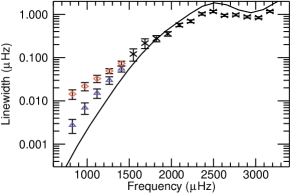
Figure 3: A comparison between observed, modelled and extrapolated linewidths. The solid line represents the modelled linewidths, the black crosses represent the linewidths found by fitting BiSON data, the red diamonds show the widths found using extrapolation method 1 and the blue triangles show the widths found using extrapolation method 2.

The top panel of Figure 4 shows a comparison between the model, observed and extrapolated powers. As we are interested in the frequency dependence of the power the model powers have been scaled to ensure that the maximum model power and the maximum observed power are equal. The model powers decrease less rapidly than the powers observed in the BiSON data. Therefore the powers estimated by both method 1 and method 2 are smaller than the model powers at low frequencies. However, this is understandable as the model widths decrease more rapidly than the observed widths. Chaplin et al. (2005) note that the model widths are too narrow at low frequencies, which implies that the extrapolations performed tend in the right direction.

It is also of interest to find the model powers using the observed widths. The bottom panel Figure 4 shows that using the observed widths produces a far better agreement with the powers observed in the BiSON data. This indicates that the majority of the discrepancy between the observed and model powers seen in the top panel of Figure 4 is due to the smaller model widths. The extrapolated powers also appear to agree better with the model values calculated using the observed widths (bottom panel of Figure 4). However, it is difficult to tell which extrapolation method produces the best agreement with the model powers. Also plotted in the bottom panel of Figure 4 are the model powers that are found when the widths estimated by both extrapolation methods are used. The agreement between the extrapolated powers and the model powers is poor when method 1 is used. However, the agreement between the extrapolated and model powers is better when method 2 is used.

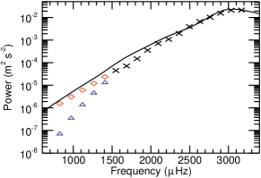
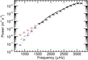
Figure 4: Top panel: A comparison between the observed, modelled and extrapolated powers. The solid line represents the modelled powers, the black crosses represent the powers found by fitting BiSON data, the red diamonds show the powers found using extrapolation method 1 and the blue triangles show the powers found using extrapolation method 2. Bottom panel: A comparison between the observed, modelled and extrapolated powers, however the model powers have been found using the observed widths. The symbols and lines have the same definitions as in the top panel. Also plotted are the model powers found using the widths estimated by extrapolation method 1 and the model powers calculated using the widths extrapolated using method 2.

3 Simulating the modes

In this section we describe how we made artificial p-mode timeseries. These timeseries were analyzed, and results on detections of their artificial modes compared with the results of Broomhall et al. (2007), on real p-mode data. In Broomhall et al. BiSON and GOLF frequency-amplitude spectra were searched for coincident prominent structures that occurred at the same frequency in each spectrum. Here we needed to simulate pairs of timeseries, which both contained the signal from a mode and normally distributed noise. The statistical tests described in Broomhall et al. (2007) were then applied to the simulated data to determine how often the simulated modes could be detected.

Modes of a given frequency and lifetime (width) were simulated by randomly exciting an oscillator that was damped over the correct timescale. The damping time was predicted using equation 1 and the extrapolations described in Section 2 for linewidth. The simulations produced timeseries that contained the signal from a simulated mode. The total power of the simulated mode was scaled to the power predicted by the simulations.

Two timeseries containing normally distributed random noise were created. The signal from two sets of contemporaneous real Sun-as-a-star data taken by different instruments, such as BiSON and GOLF, contains some coherent noise. This noise is solar in origin and comes from the solar granulation. The level of coherent noise is frequency dependent and at around $1000\,\rm\mu Hz$ the coherency between BiSON and GOLF data is $\sim 0.1$. Therefore 10% of the noise in the two simulated timeseries was set so it was common to both sets of simulated data. The timeseries containing the signal from the simulated mode was then added to each noise timeseries.

Solar modes are excited stochastically by turbulence in the convection zone, which is caused by the solar granulation. As the coherent noise in two sets of Sun-as-a-star data is from the granulation it is possible that the coherent noise found between the BiSON and GOLF data is also correlated to the amplitude of excitation of the mode. In the simulations the amplitude of the excitation was determined by a normally distributed array. For some of the simulations the correlated noise that was added to the simulated data was taken to be the array that determined the amplitude of the excitation of the mode. Simulations were also performed when the noise that was coherent between the two simulated sets of data was independent of the amplitude of excitation of the mode.

The simulations have been performed for the $l=0$ modes between $\sim 800$ and $\sim 1450\,\rm\mu Hz$, the extrapolated properties of which are given in Tables 2 and 3. The timeseries were simulated to contain 2,211,120 points with a cadence of 120s to be consistent with the sets of BiSON and GOLF data used in Broomhall et al. (2007). The simulated and BiSON timeseries cover the same length in time ($\sim 8.5\,\rm yrs$), despite having different cadences and containing a different number of points. This means that the power of a mode in the simulated and observed timeseries is the same. Furthermore, the number of frequency bins that cover the width of a mode in the simulated frequency-power spectra is the same as in the fitted BiSON spectrum. Therefore, the height of the mode in a simulated frequency-power spectrum will be the same as the height predicted by the extrapolations. The level of noise in the simulated spectra was scaled to mimic the mean level of noise observed in the BiSON frequency-power spectrum in the $100\,\rm\mu Hz$ surrounding the frequency of the mode that was simulated.

It should be noted that we are considering low-frequency modes, which are relatively insensitive to the effects of the solar activity cycle. We would therefore not expect solar cycle effects to have a significant impact on results, and so solar cycle effects were neglected in the simulations.

Each extrapolated power and width has an error associated with it. To obtain an upper limit on the fraction of times a simulated mode could be detected Monte Carlo simulations were performed using the $\pm 1\sigma$ error values of the extrapolated widths and powers.

Once timeseries containing a mode and noise had been created several tests were performed on the resulting frequency-amplitude spectra to determine whether the mode could be detected or not. For each mode 1000 pairs of timeseries were simulated. Each pair of simulated timeseries corresponds to a different realization. The number of pairs of spectra in which a mode was detected was then counted. Various statistical tests were used to detect the modes. We will now outline each of these tests in turn.

4 Statistical Tests

The tests performed are based on the statistics described in detail in Chaplin et al. (2002) and Broomhall et al. (2007). Here we summarize the statistical tests that were used to search the simulated spectra. The simplest test involves searching for a single prominent spike that is above a given threshold level in the same bin in each of the two simulated frequency-amplitude spectra. The threshold level for detection was set at a 1 per cent chance of getting at least one false detection anywhere in $100\,\rm\mu$Hz. This level and frequency range were chosen to maintain consistency with the detection methods employed in Broomhall et al. (2007). The probability of observing such a ‘pair of spikes’ takes proper account of the level of common noise present in the two frequency-amplitude spectra as this affects the probability that any detection is due to noise. A detection was considered to have been made if it was positioned within one linewidth of the input frequency. The linewidths were determined by the extrapolated values and so varied between modes. As the modes are damped it is possible to take advantage of the width the mode may exhibit in frequency. Furthermore, if the frequency of a mode is not commensurate with the frequency bins of the spectrum the power of the mode may be spread over more than one bin. The second test involves searching for two prominent spikes in the same consecutive frequency bins of each frequency-amplitude spectrum. Both spikes must lie within one peak width of the mode’s input frequency for a detection to be counted. The third test performed also searched for two prominent spikes but this time the spikes did not need to be in consecutive bins. These two spikes are known as a two-spike cluster. The bins occupied by the two spikes could lie up to twice the predicted peak width apart. However each spike had to lie less than one linewidth from the mode’s input frequency for a detection to be counted. The two prominent spikes in the cluster needed to be in the same bins in each frequency-amplitude spectrum. This test was then extended to search for clusters containing three, four and five prominent spikes. The highest and lowest frequency spikes in the cluster had to be separated by less than twice the width of the mode. Furthermore, each prominent spike in the cluster had to be in the same frequency bin in each frequency-amplitude spectrum. All spikes in the clusters needed to lie within one linewidth of the mode’s input frequency for a detection to be counted.

The simulated spectra were searched to determine how often these statistical tests were passed for each mode. The results of these tests will now be described.

5 Results of the Simulations

Figure 5 shows the fraction of the 1000 simulations that were performed in which the mode being simulated was detected when looking for a single spike in the same bin in each spectrum. The results show that using the parameters predicted by method 1 leads to more detections than the parameters estimated by method 2. This is expected as the powers predicted by method 1 are significantly larger than the powers predicted by method 2. More detections are made when the noise that is coherent between the two sets of data is also correlated to the amplitude of the excitation of the mode. This is also understandable. If, for example, at a point in time the level of solar noise is larger than average the amplitude of the excitation of the mode will also be larger than average enabling it to potentially remain distinguishable from the noise. However, all of the simulations that use the extrapolated values predict that the number of detections at low frequencies will be small. Also plotted on Figure 5 are the results of simulations performed using the model widths and powers predicted by the stochastic excitation model described in Chaplin et al. (2005). The model powers have been found using the model widths rather than the observed widths. Clearly more detections are made when the model parameters are used.

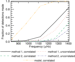
Figure 5: Comparison between the fraction of modes detected when different input parameters were used.

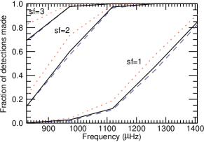
(a) Method 1

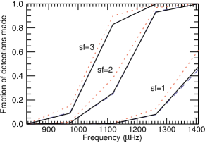
(b) Method 2

Figure 6: Results of searching for a single spike when the noise is correlated with the excitation amplitude. The black solid lines show the results for the actual extrapolated values. The red dashed lines show the results when the maximum power and minimum widths are used in the simulations. The blue dashed line shows the results of the simulations that used the maximum powers and the maximum widths. The three clusters of lines are present as for each set of parameters the power was scaled by a different amount. The clusters labelled sf=1 represent the true predicted values. The clusters labelled sf=2 show the results when the power was increased by a factor of 2 and the clusters labelled sf=3 are the results when the power was increased by a factor of 3.

Figure 6 plots results from the spike tests where the coherent noise was correlated to the mode excitation. Each panel of Figure 6 shows three clusters of lines. The solid, black lines in the clusters labelled sf=1 represent the results from simulations where the power and width of the input mode were predicted by the respective extrapolation methods. The results show that the number of detections decreases rapidly as we move to lower frequencies. As each of the statistical tests are looking for prominent spikes it is the height the mode exhibits in the frequency-amplitude/power spectra that determines whether or not it can be detected. The height of a mode in a frequency-power spectrum is proportional to $V^{2}/\Delta$ (see equation 2). The upper limit on the number of detections is given by the case when the maximum power and minimum width is used. Using the maximum power and minimum width means that the height of the mode, $H$, is, potentially, larger and so the signal-to-noise ratio of the mode should be increased. It is therefore understandable that using the maximum power and minimum width leads to more detections. When the simulations were performed using the maximum width the power is spread over a larger number of bins and so this negates the effect on the signal-to-noise ratio of the mode of increasing its power.

Simulations were also performed to investigate the effect of increasing the observed signal-to-noise ratio. The power given to each simulated mode was increased by factors of 2 (labelled sf=2 in each panel of Figure 6) and 3 (labelled sf=3 in each panel of Figure 6). This significantly increases the number of detections made at low frequencies. The fraction of spectra in which the $l=0$, $n=6$ mode was detected when the scale factor was 1 was at most 0.05. However, the fraction of detections made when the scale factor was 2 was 0.60 and when the scale factor was 3 the fraction of simulated spectra in which the $l=0$, $n=6$ mode was detected was 0.98.

6 Discussion

Clearly the visibility of the modes drops off at low frequencies. The most optimistic results are achieved when the extrapolation is performed using method 1 and the common noise is correlated to the amplitude of the excitation of the mode. Clearly more detections are made when the stochastic excitation model parameters are used. However, these results can only be treated as an upper limit as we have already seen that the model underestimates the widths of the modes. This not only leads to the power of the modes being overestimated but also means that the height of a mode is increased, and so a mode is more likely to be detected.

For both extrapolation methods, irrespective of whether the noise is correlated or uncorrelated with the excitation amplitude, the fraction of detections at $\sim 1000\,\rm\mu Hz$ is less than 0.1. On the assumption that method 1 produces a more accurate prediction of the mode’s powers and widths than method 2 the simulations imply that if the power signal-to-noise ratio can be increased by a factor of 2 a significantly higher proportion of modes could be detected. It would therefore be beneficial to continue efforts to try and improve the quality of the data further.

The total background continuum is a combination of instrumental noise, solar noise and, for Earth-based instruments such as the BiSON network, a small amount of atmospheric noise. If the atmospheric and instrumental noise can be reduced this would increase the signal-to-noise ratio of a mode, making it easier to detect. The limiting factor to the improvement that can be made to the data quality is the amount of solar noise present. However, the mean power of the BiSON data is always more than twice the power of solar noise predicted by the Harvey model and the characteristic parameters for the granulation found by [Elsworth et al. (1994)]. Therefore it is theoretically possible to significantly reduce the level of noise in this frequency range.

It is possible to compare the results of these simulations to the observed candidates found in Broomhall et al. (2007). According to the simulations the $l=0$, $n=9$ mode at $\sim 1407\,\rm\mu Hz$ should be detected in the vast majority of spectra and this mode is observed to be very prominent in the BiSON and GOLF data used in Broomhall at al.. The $l=0$, $n=8$ mode at $\sim 1263\,\rm\mu Hz$ is also detected by Broomhall et al.. The simulations indicate that the fraction of time that this mode should be detected is at least 0.6. The $l=0$, $n=7$ mode at $\sim 1118\,\rm\mu Hz$ and the $l=0$, $n=5$ mode at $\sim 825\,\rm\mu Hz$ are not detected in the BiSON and GOLF data used in Broomhall et al.. The fraction of simulated spectra in which the $l=0$, $n=7$ mode was detected was, at most, 0.35, while the fraction of simulations in which the $l=0$, $n=5$ mode was detected was less than 0.06. Therefore it is reasonable to expect that the modes might not be detected in the BiSON and GOLF data.

It should of course be noted here that all of these results are based on the assumption that the simple relationships for the mode powers and widths observed in well-defined modes are still valid at low frequencies. The solar excitation model suggests that this may not be an unreasonable assumption, although it is difficult to determine which extrapolation method predicts the lifetimes and powers more accurately.

The $l=0$, $n=6$ mode is significantly more prominent in the observations than the simulations. Therefore this mode will now be considered in more detail.

6.1 The $l=0$, $n=6$ mode

The $l=0$, $n=6$ mode is observed to be prominent in Sun-as-a-star data. However, some modes with higher frequencies remain undetected. The most optimistic simulations imply that the fraction of spectra in which the $l=0$, $n=6$ mode should be detected is less than 0.05. In the simulations performed here, for method 1, with noise correlated to the amplitude of the excitation, the average simulated signal-to-noise ratio in amplitude was $\sim 2.1$. However, the observed amplitude signal-to-noise ratio in the GOLF and BiSON data examined in Broomhall et al. (2007) was greater than $3.4$. In fact, the fraction of simulations in which the signal-to-noise ratio of the mode was greater than 3.4 was 0.014. Therefore the simulations poorly represent the observed properties of this mode. It should be noted that the amplitude signal-to-noise ratio of other modes that were detected in Broomhall et al. are well represented by the simulations in this paper. For example, the $l=0$, $n=9$ mode was observed to have a signal-to-noise ratio of 3.1 while the average signal-to-noise ratio produced by the simulations ranged from 2.9 to 3.7 depending on which extrapolation method was used and whether the noise was correlated to the excitation amplitude.

When the mean amplitude signal-to-noise ratio of the simulated $l=0$, $n=6$ mode was set as 3.4 the fraction of spectra in which the mode was detected increased to $\sim 0.6$. A signal-to-noise ratio of 3.4 is $\sim 3\sigma$ from the mean amplitude signal-to-noise found in the original simulations where extrapolation method 1 (ln-linear) is used and the noise is correlated to the excitation amplitude. Therefore, the simulations and the observations are not so different that new physics is required to explain the observations. It is more likely that at some point in time the mode has been randomly excited to a larger amplitude because of the stochastic nature of mode excitation.

References

- [Appourchaux et al. (2000)] Appourchaux, T., Fröhlich, C., Andersen, B., Berthomieu, G., Chaplin, W. J., Elsworth, Y., Finsterle, W., Gough, D. O., et al.: 2001, ApJ 538, 401
- [Broomhall et al. 2007] Broomhall, A. M., Chaplin, W. J., Elsworth, Y., Appourchaux, T.: 2007, MNRAS 379, 2
- [Chaplin et al. 2002] Chaplin, W.J., Elsworth, Y., Isaak, G.R., Marchenkov, K.I., Miller, B.A., New, R., Pinter, B.: 2002, MNRAS 336, 979
- [Chaplin et al. 2005] Chaplin, W. J., Houdek, G., Elsworth, Y., Gough, D. O., Isaak, G. R., New, R.: 2005, MNRAS 360, 859
- [Elsworth et al. (1994)] Elsworth, Y., Howe, R., Isaak, G.R., McLeod, C.P., Miller, B.A., New, R., Speake, C.C., Wheeler, S.J.: 1994, MNRAS 269, 529
- [Fletcher (2007)] Fletcher, S. T.: 2007, PhD thesis, University of Birmingham
- [García et al. 2001] García, R. A., Régulo, C., Turck-Chièze, S., Bertello, L., Kosovichev, A. G., Brun, A. S., Couvidat, S., Henney, C. J., et al.: 2001, Sol. Phys. 200, 361
- [Houdek et al. (1999)] Houdek, G., Balmforth, N. J., Christensen-Dalsgaard, J., Gough, D. O.: 1999, A&A 351, 582
- [(Turck-Chièze et al. 2001)] Turck-Chièze, S., Couvidat, S., Kosovichev, A. G., Gabriel, A. H., Berthomieu, G., Brun, A. S., Christensen-Dalsgaard, J., García, R. A., et al.: 2001, ApJ 555, L69