Superconductivity from four Fermion complexes

Abstract

Superconductivity is studied for a fermionic system with attractive four-body interaction. Applying a Green function approach, the gap equation is derived. From the solution, the transition temperature is calculated. Under the condition that the respective coupling constants are comparable, the transition temperature of four-fermion complexes is considerably larger than the corresponding BCS value.

I Introduction

About fifty years ago, the development of the BCS theory bcs and its overwhelming success in physics and application was a breakthrough in modern theoretical physics. This theory provides basic insight into superconductivity from a quantum-mechanical point of view. According to the BCS mechanism, the superconducting phase is due to the condensation of bosonic quasi-particles, called Cooper pairs, which are created from Fermions that experience an effective weak attractive interaction. An essential ingredient of the BCS theory was the observation Bardeen that there could be a phonon-mediated attraction between electrons in some metals at low temperatures. This effective force acts at longer distances than the short-range screened Coulomb interaction. In the simplified version of the model bcs , the attractive interaction is constant in a narrow energy region (of the order of the Debye energy $\hbar\omega_{D}$) around the Fermi energy and zero outside. As the extent of a Cooper pair exponentially increases with decreasing coupling, a large number of Cooper pair wave functions usually overlap with each other. In the extreme limit of vanishing attractive coupling $g_{2}$, the non-perturbative BCS theory becomes exact.

The attractive interaction between fermions may originate from quite different sources. Since the effective attraction could be due not only to phonons but also to other bosonic excitations, the BCS approach has been successfully applied to many quite different research fields. Unfortunately, the basic physics of high-temperature superconductivity Bednorz does not fit into any weak-coupling schema and therefore also not into the BCS theory. The measured transition temperature $T_{c}$ in cuprates, which can reach 160 K, cannot be derived from realistic BCS calculations.

Regardless of this disadvantage, it is not exaggerated to state that the BCS theory has deepened our understanding of many-body effects in the quantum world. The non-perturbative character of the approach, as revealed by the highly nonlinear dependence of the transition temperature or the gap energy on the coupling constant $g_{2}$, expresses the fact that the superconducting phase is to be understood as a complex many-body phenomenon, to which an infinite number of particular particle correlations contribute. In addition, the resulting Cooper pairs, which carry the superconducting current, do not exist as spatially separated entities but are collected into large drops, in which novel collective quantum effects could exist in principle. However, the BCS approach focuses on pair correlations meaning that the behavior of more than two highly correlated quantum objects is described by two-body interactions between all possible pairs. The question arises whether this first approximation is exhaustive for the description of many-body quantum effects. In fact, many-body interactions have been studied in different research areas like nuclear, atomic, and condensed matter physics. The main reason usually is the treatment of cluster effects created by an ensemble of strongly correlated particles (especially self-consistent cluster approximations Elliott ). In the field of nuclear physics there is growing evidence that three-body forces exist among the nucleons inside atomic nuclei. In condensed-matter physics, many-body effects of trions were studied Comb and three-body forces were shown to dominate the Cauchy discrepancies in the second and third order elastic constants of Copper. Cousins Three-body contributions to the interatomic potential also modify many properties of the liquid and solid phases of ⁴He atoms. Ujevic Even a spectacular result have been reported in the field of many-body interaction Date namely that a $D$-dimensional Hamiltonian with two- and three-body interactions has a unique string-like ground state, when the strength of the three-body coupling exceeds a critical value. In a recent study of the Bose-Einstein condensate-BCS crossover in fermionic systems Mora , the Schrödinger equation for four attractively interacting fermions was solved by applying Bethe ansatz techniques. The solution reveals a robust four-fermion cluster that is not broken by collision and does not couple to additional fermionic states.

The mentioned papers initiated a study of the rich and interesting quantum physics that refers to many-body interaction. The objective of the present paper is to contribute to this fascinating field by treating a BCS-like instability in an electron gas with four fermion coupling.

II Basic approach

The BCS theory is based on the pair approximation with an effective particle-particle coupling that is attractive and phonon mediated. Similarly, it is conceivable that also a cluster of three fermions is glued together by an attracting three-body coupling. However, due to its fermionic character, these aggregates are not expected to form a condensate. One needs two or four fermion complexes for their transmutation into boson-like objects, which could give rise to a phase transition to a superconductor. Here, we focus on an instability, which is due to the conglomerate of four fermions described by an effective potential $v$. In order to concentrate on possible instabilities in the system, both pair- and higher-order particle interactions are not taken into account. Therefore, we start from the model Hamiltonian

$$H=\sum\limits_{s}\int d{\bm{r}}\psi_{s}^{{\dagger}}({\bm{r}},t)\left[-\frac{\hbar^{2}}{2m}\triangle_{\bm{r}}+V({\bm{r}})\right]\psi_{s}({\bm{r}},t)$$ (1)

$$+\sum\limits_{\{s_{i}\}}\int\{d{\bm{r}_{i}}\}\psi_{s_{1}}^{{\dagger}}({\bm{r}_{1}},t)\psi_{s_{2}}^{{\dagger}}({\bm{r}_{2}},t)\psi_{s_{3}}^{{\dagger}}({\bm{r}_{3}},t)\psi_{s_{4}}^{{\dagger}}({\bm{r}_{4}},t)$$

$$\times v({\bm{r}_{1}},{\bm{r}_{2}},{\bm{r}_{3}},{\bm{r}_{4}})\psi_{s_{4}}({\bm{r}_{4}},t)\psi_{s_{3}}({\bm{r}_{3}},t)\psi_{s_{2}}({\bm{r}_{2}},t)\psi_{s_{1}}({\bm{r}_{1}},t),$$

where $V({\bm{r}})$ and $m$ denote the crystal potential and the effective mass, respectively. Fermions with spin $s$ are created [annihilated] by the operators $\psi_{s}^{{\dagger}}({\bm{r}},t)$ [$\psi_{s}({\bm{r}},t)$]. Furthermore, the abbreviation $\{d{\bm{r}_{i}}\}=d{\bm{r}_{1}}d{\bm{r}_{2}}d{\bm{r}_{3}}d{\bm{r}_{3}}$ is used. The one-particle Green function satisfies the equation of motion Baym

$$\biggl{\{}i\hbar\frac{\partial}{\partial t_{1}}+\frac{\hbar^{2}}{2m}\triangle_{\bm{r}_{1}}-V({\bm{r}_{1}})-U(1)\biggl{\}}G(1,1^{\prime};U)=\delta(1-1^{\prime})$$ (2)

$$-i\hbar^{3}\int d\overline{2}d\overline{3}d\overline{4}V(1,\overline{2},\overline{3},\overline{4})G(1,\overline{2},\overline{3},\overline{4};1^{\prime},\overline{2}^{+},\overline{3}^{+},\overline{4}^{+};U),$$

with $U(1)\equiv U_{s}({\bm{r}},t)$ being an arbitrary auxiliary function. In this equation, the usual notation is used, e.g. $\overline{2}^{+}=\{{\bm{r}_{\overline{2}}},t_{\overline{2}}+i\varepsilon,s_{\overline{2}}\}$ with $\varepsilon\rightarrow 0$. As Eq. (2) is not closed, it must be supplemented by an equation for the four-particle Green function and so on. This hierarchy is alternatively deduced from the generating functional $G[\lambda,\eta]$

$$G(1,\dots,n;1^{\prime},\dots,n^{\prime};U)=\left.\frac{\delta}{\delta\eta(n^{\prime})}\dots\frac{\delta}{\delta\eta(1^{\prime})}\frac{\delta}{\delta\lambda(1)}\dots\frac{\delta}{\delta\lambda(n)}G[\lambda,\eta]\right|_{\lambda=\eta=0},$$ (3)

by taking functional derivatives with respect to the Grassmannian source fields $\lambda$ and $\eta$ before they are set equal to zero. Expressing Eq.(2) by a functional differential equation

$$\biggl{\{}i\hbar\frac{\partial}{\partial t_{1}}+\frac{\hbar^{2}}{2m}\triangle_{\bm{r}_{1}}-V({\bm{r}_{1}})-U(1)\biggl{\}}\frac{\delta}{\delta\lambda(1)}G[\lambda,\eta]=\eta(1)G[\lambda,\eta]$$ (4)

$$-i\hbar^{3}\int d\overline{2}d\overline{3}d\overline{4}V(1,\overline{2},\overline{3},\overline{4})\frac{\delta}{\delta\eta(\overline{4}^{+})}\frac{\delta}{\delta\eta(\overline{3}^{+})}\frac{\delta}{\delta\eta(\overline{2}^{+})}\frac{\delta}{\delta\lambda(\overline{2})}\frac{\delta}{\delta\lambda(\overline{3})}\frac{\delta}{\delta\lambda(\overline{4})}\frac{\delta}{\delta\lambda(1)}G[\lambda,\eta],$$

the coupled set of equations for the Green functions is easily obtained by calculating additional functional derivatives of desired order. At this stage, it is recommended to introduce the generating functional $G_{c}[\lambda,\eta]$ for the connected parts of many-particle Green functions via the equation

$$G[\lambda,\eta]=\exp\left\{G_{c}[\lambda,\eta]\right\}.$$ (5)

For instance, for the one- and two-particle functions, the relationship

$$G(1,1^{\prime};U)=G_{c}(1,1^{\prime};U)$$ (6)

$$G(1,2;1^{\prime},2^{\prime};U)=G_{c}(1,2;1^{\prime},2^{\prime};U)+G(1,1^{\prime};U)G(2,2^{\prime};U)-G(1,2^{\prime};U)G(2,1^{\prime};U),$$ (7)

is derived, from which it is concluded that the correlated two-particle Green function does not enclose the Hartree-Fock contributions. It is a general property that the correlated Green functions vanish, when the interaction is absent so that the hierarchy is suitably truncated by disregarding higher-level many-particle contributions described by correlated Green functions.

Inserting the correlated four-particle Green function into Eq. (2), we obtain an equation, in which numerous terms appear that represent various kinds of four-fermion scattering. It is in line with our approach, which looks for a BCS-like instability for four fermion complexes, to neglect all two- and three-particle connected Green functions. The remaining conglomerate of one-particle Green functions is collected into an effective function $G_{0}(1,1^{\prime};U)$ [in the pair approximation, which is the basis of the BCS theory, $G_{0}$ is given by the Hartree-Fock Green function] so that we obtain

$$G(1,1^{\prime};U)= G_{0}(1,1^{\prime};U)-i\hbar^{3}\int d\overline{1}d\overline{2}d\overline{3}d\overline{4}G_{0}(1,\overline{1};U)V(\overline{1},\overline{2},\overline{3},\overline{4})$$ (8)

$$\times G_{c}(\overline{1},\overline{2},\overline{3},\overline{4};1^{\prime},\overline{2}^{+},\overline{3}^{+},\overline{4}^{+};U).$$

This result is complemented by the equation of motion for the eight-point Green function, which is derived from Eqs. (4) and (5). The handling of this rather complicated integral equation is guided by the well established pair approximation Puff ; Kleinert that leads to the BCS theory. In accordance with the BCS reasoning, we focus on the homogeneous Cooper channel, in which the connected four-particle function is self-consistently determined from

$$G_{c}(1,2,3,4;1^{\prime},2^{\prime},3^{\prime},4^{\prime};U)=i\hbar^{3}\int d\overline{1}d\overline{2}d\overline{3}d\overline{4}G_{0}(1,\overline{1};U)V(\overline{1},\overline{2},\overline{3},\overline{4})$$ (9)

$$\times G(2,\overline{2}^{+};U)G(3,\overline{3}^{+};U)G(4,\overline{4}^{+};U)G_{c}(\overline{1},\overline{2},\overline{3},\overline{4};1^{\prime},2^{\prime},3^{\prime},4^{\prime};U).$$

Figure 1: Diagrammatic representation of the Cooper channel. The wavy lines represent the four-body interaction.

A diagrammatic representation of the scattering contribution is shown in Fig. 1. The basic set of Eqs. (8) and (9) extends the BCS theory Puff ; Kleinert to fermions coupled via a four-body potential. The solution of these equations is facilitated by a Fourier transformation in the time domain. Introducing the Matsubara frequencies ($z_{\nu}=i\pi\nu/(\hbar\beta)+\mu/\hbar$, $\nu=\pm 1,\pm 3,\dots$ and $\omega_{n}=i\pi n/(\hbar\beta)+4\mu/\hbar$, $n=0,\pm 2,\dots$ with $\mu$ being the chemical potential and $\beta=1/k_{B}T$), the Fourier transformation is defined by

$$G_{c}(1,2,3,4;1^{\prime},2^{\prime},3^{\prime},4^{\prime};U)=\left(\frac{i}{\hbar\beta}\right)^{7}\sum\limits_{\{\nu_{i}\}}\sum\limits_{\{\nu_{i}^{\prime}\}}\sum\limits_{n}G_{c}(\{x_{i}\};\{x_{i}^{\prime}\}|\{z_{\nu_{i}}\};\{z_{\nu_{i}^{\prime}}\}|\omega_{n})$$

$$\times\exp\left[-iz_{\nu_{1}}t_{1}-iz_{\nu_{2}}t_{2}-iz_{\nu_{3}}t_{3}-i(\omega_{n}-z_{\nu_{1}}-z_{\nu_{2}}-z_{\nu_{3}})t_{4}\right]$$

$$\times\exp\left[iz_{\nu_{1}^{\prime}}t_{1}^{\prime}+iz_{\nu_{2}^{\prime}}t_{2}^{\prime}+iz_{\nu_{3}^{\prime}}t_{3}^{\prime}+i(\omega_{n}-z_{\nu_{1}^{\prime}}-z_{\nu_{2}^{\prime}}-z_{\nu_{3}^{\prime}})t_{4}^{\prime}\right],$$ (10)

where the spin and spatial coordinates are expressed by $\{x_{i}\}=x_{1},x_{2},x_{3},x_{4}$ with $x_{j}={\bm{r}_{j}},s_{j}$ and $\{z_{\nu_{i}}\}=z_{\nu_{1}},z_{\nu_{2}},z_{\nu_{3}}$. When treating the Fourier transformed basic Eqs. (8) and (9), the following functions occur

$$G_{c}(\{x_{i}\};\{x_{i}^{\prime}\}|\{z_{\nu_{i}^{\prime}}\}|\omega_{n})=\left(\frac{i}{\hbar\beta}\right)^{3}\sum\limits_{\{\nu_{i}\}}G_{c}(\{x_{i}\};\{x_{i}^{\prime}\}|\{z_{\nu_{i}}\};\{z_{\nu_{i}^{\prime}}\}|\omega_{n}),$$ (11)

$$G_{c}(\{x_{i}\};\{x_{i}^{\prime}\}|\omega_{n})=\left(\frac{i}{\hbar\beta}\right)^{6}\sum\limits_{\{\nu_{i}\},\{\nu_{i}^{\prime}\}}G_{c}(\{x_{i}\};\{x_{i}^{\prime}\}|\{z_{\nu_{i}}\};\{z_{\nu_{i}^{\prime}}\}|\omega_{n}),$$ (12)

$$\Delta(\{x_{i}\};\{x_{i}^{\prime}\}|\omega_{n})=v(\{{\bm{r}_{i}}\})v(\{{\bm{r}_{i}^{\prime}}\})G_{c}(\{x_{i}\};\{x_{i}^{\prime}\}|\omega_{n}).$$ (13)

The integral equation for the gap function $\Delta$ in the representation with Matsubara frequencies is straightforwardly obtained from Eq. (9)

$$\Delta(\{x_{i}\};\{x_{i}^{\prime}\}|\omega_{n})=-i\hbar^{3}v({\bm{r}_{1}},\dots,{\bm{r}_{4}})\int\{dx_{\overline{i}}\}\left(\frac{i}{\hbar\beta}\right)^{3}\sum\limits_{\{\nu_{i}\}}G_{0}(x_{1},x_{\overline{1}},z_{\nu_{1}})G(x_{2},x_{\overline{2}},z_{\nu_{2}})$$

$$\times G(x_{3},x_{\overline{3}},z_{\nu_{3}})G(x_{4},x_{\overline{4}},\omega_{n}-z_{\nu_{1}}-z_{\nu_{2}}-z_{\nu_{3}})\Delta(\{x_{\overline{i}}\};\{x_{i}^{\prime}\}|\omega_{n}).$$ (14)

To derive the corresponding Fourier transformed version of Eq. (8), we account for the symmetry property

$$G_{c}(\{x_{i}\};\{x_{i}^{\prime}\}|\{z_{\nu_{i}}\};\{z_{\nu_{i}^{\prime}}\}|\omega_{n})=-G_{c}^{*}(\{x_{i}^{\prime}\};\{x_{i}\}|\{z_{\nu_{i}^{\prime}}^{*}\};\{z_{\nu_{i}}^{*}\}|\omega_{n}^{*}),$$ (15)

which leads to an alternative formulation of Eq. (14). Inserting this gap function into Eq. (8) and performing a spatial Fourier transformation by using a definition similar to Eq. (10), we obtain

$$G({\bm{k}},z_{\nu})=G_{0}({\bm{k}},z_{\nu})+\hbar^{6}G_{0}^{2}({\bm{k}},z_{\nu})\left(\frac{i}{\hbar\beta}\right)\sum\limits_{{\bm{q}},n}\Delta({\bm{q}},\omega_{n})$$ (16)

$$\times\left(\frac{i}{\hbar\beta}\right)^{2}\sum\limits_{{\bm{k}_{1}},\nu_{1}}\sum\limits_{{\bm{k}_{2}},\nu_{2}}G({\bm{k}_{1}},z_{\nu_{1}})G({\bm{k}_{2}},z_{\nu_{2}})G({\bm{q}}-{\bm{k}}-{\bm{k}_{1}}-{\bm{k}_{2}};\omega_{n}-z_{\nu}-z_{\nu_{1}}-z_{\nu_{2}}),$$

where the new gap function is given by

$$\Delta({\bm{q}},\omega_{n})=\sum\limits_{\{s_{i}\}}\sum\limits_{\{{\bm{k}}_{i}\}}\sum\limits_{\{{\bm{k}}_{i}^{\prime}\}}\Delta_{\{s_{i}\},\{s_{i}\}}(\{{\bm{k}_{i}}\},\{{\bm{k}_{i}^{\prime}}\}|{\bm{q}},\omega_{n}).$$ (17)

In the derivation, it was considered $G_{ss^{\prime}}=\delta_{ss^{\prime}}G$, which dictates the spin dependence of the gap function. The basic Eq. (16) for the one-particle Green function provides an obvious extension of the BCS singlet state description. Puff ; Kleinert Similarly, we obtain for the gap equation the following Fourier-transformed version

$$\Delta(\{{\bm{k}_{i}}\};\{{\bm{k}_{i}}^{\prime}\}|{\bm{q}},\omega_{n})=-i\hbar^{3}\sum\limits_{\{{\bm{k}_{\overline{i}}}\}}v({\bm{k}_{1}}-{\bm{k}_{\overline{1}}},{\bm{k}_{1}}-{\bm{k}_{\overline{1}}}+{\bm{k}_{2}}-{\bm{k}_{\overline{2}}}$$

$$,{\bm{k}_{1}}-{\bm{k}_{\overline{1}}}+{\bm{k}_{2}}-{\bm{k}_{\overline{2}}}+{\bm{k}_{3}}-{\bm{k}_{\overline{3}}})\left(\frac{i}{\hbar\beta}\right)^{3}\sum\limits_{\{\nu_{i}\}}G_{0}({\bm{k}_{\overline{1}}},z_{\nu_{1}})G({\bm{k}_{\overline{2}}},z_{\nu_{2}})G({\bm{k}_{\overline{3}}},z_{\nu_{3}})$$

$$\times G({\bm{q}}-{\bm{k}_{\overline{1}}}-{\bm{k}_{\overline{2}}}-{\bm{k}_{\overline{3}}},\omega_{n}-z_{\nu_{1}}-z_{\nu_{2}}-z_{\nu_{3}})\Delta(\{{\bm{k}_{\overline{i}}}\};\{{\bm{k}_{i}}^{\prime}\}|{\bm{q}},\omega_{n}).$$ (18)

In the spirit of the BCS theory Puff ; Kleinert , Eqs. (16) and (18) are solved in the limit ${\bm{q}}={\bm{0}}$ and $n=0$, which is an approximation concerning the effective bosonic excitation composed of four particles. In addition, it is assumed that the effective attraction is given by a contact interaction, which is confined to a narrow shell of width $2\hbar\omega_{D}$ around the Fermi energy. Introducing the new abbreviations ${\bm{k}_{2}}+{\bm{k}_{3}}={\bm{q}}$ and $z_{\nu_{2}}+z_{\nu_{3}}=\omega_{m}$, we obtain the final set of coupled equations

$$G({\bm{k}},z_{\nu})=G_{0}({\bm{k}},z_{\nu})+\Delta\hbar^{6}G_{0}^{2}({\bm{k}},z_{\nu})\left(\frac{i}{\hbar\beta}\right)\sum\limits_{{\bm{q}},m}u({\bm{q}},\omega_{m})G^{*}({\bm{k}}+{\bm{q}},z_{\nu}+\omega_{m}),$$ (19)

$$-i\hbar^{3}g_{4}\left(\frac{i}{\hbar\beta}\right)\sum\limits_{{\bm{q}},m}u({\bm{q}},\omega_{m})\left(\frac{i}{\hbar\beta}\right)\sum\limits_{{\bm{k}},\nu}G_{0}({\bm{k}},z_{\nu})G^{*}({\bm{k}}+{\bm{q}},z_{\nu}+\omega_{m})=1,$$ (20)

$$u({\bm{q}},\omega_{m})=\left(\frac{i}{\hbar\beta}\right)\sum\limits_{{\bm{k}_{1}},\nu_{1}}G({\bm{k}_{1}},z_{\nu_{1}})G({\bm{q}}-{\bm{k}_{1}},\omega_{m}-z_{\nu_{1}}),$$ (21)

which generalizes the BCS theory to a fermionic system with four-body interaction. These equations allow a detailed description of the superconducting phase of the considered cluster model. Formally, Eqs. (19) and (20) reduce to the basic BCS equations, when the function $u({\bm{q}},\omega_{m})$ is replaced by $-i\hbar\beta\delta_{m,0}\delta_{{\bm{q}},{\bm{0}}}$.

III Transition temperature

The internal structure of the four-particle cluster is mainly accounted for by the function $u({\bm{q}},\omega_{n})$, which has a bosonic character. To study its influence in more detail, let us treat the transition temperature $T_{c}$, at which the gap energy $\Delta$ vanishes. For the calculation of $T_{c}$, the self-consistent one-particle Green function $G$ is given by $G_{0}$, for which, in analogy to the BCS approach, the simple expression

$$G_{0}({\bm{k}},z_{\nu})=\frac{1}{\hbar z_{\nu}-\varepsilon_{{\bm{k}}}},$$ (22)

is adopted. $\varepsilon_{\bm{k}}$ denotes the kinetic energy $\hbar^{2}{\bm{k}^{2}}/2m$. For the function $u({\bm{q}},\omega_{n})$, we immediately obtain

$$u({\bm{q}},\omega_{l})=\frac{i}{\hbar}\sum\limits_{\bm{k}}\frac{n_{F}(\xi_{{\bm{k}}})+n_{F}(\xi_{{\bm{q}}-{\bm{k}}})-1}{i\omega_{l}-\xi_{{\bm{k}}}-\xi_{{\bm{q}}-{\bm{k}}}},$$ (23)

with the Fermi distribution function $n_{F}$, $i\omega_{l}=2\pi il/\beta_{c}$, $\beta_{c}=1/k_{B}T_{c}$, and $\xi_{{\bm{k}}}=\varepsilon_{\bm{k}}-\mu$. Inserting this result into Eq. (20), we obtain the gap equation

$$g_{4}\sum\limits_{\bm{k}_{1},\bm{k}_{2}}\sum\limits_{\bm{q}}\left[n_{F}(\xi_{\bm{k}_{1}+\bm{q}})+n_{F}(\xi_{\bm{k}_{1}})-1\right]\left[n_{F}(\xi_{\bm{k}_{2}-\bm{q}})+n_{F}(\xi_{\bm{k}_{2}})-1\right]$$

$$\times\frac{n_{B}(\xi_{\bm{k}_{1}+\bm{q}}+\xi_{\bm{k}_{1}})+n_{B}(\xi_{\bm{k}_{2}-\bm{q}}+\xi_{\bm{k}_{2}})+1}{\xi_{\bm{k}_{1}+\bm{q}}+\xi_{\bm{k}_{1}}+\xi_{\bm{k}_{2}-\bm{q}}+\xi_{\bm{k}_{2}}}=1,$$ (24)

in which the Bose distribution function $n_{B}$ and the four-body coupling $g_{4}$ appear. Let us compare this result of the BCS-like approach for four fermions, which are held together by a four-body phonon-mediated attraction, with the gap equation of the BCS theory

$$g_{2}\sum\limits_{\bm{k}}\frac{2n_{F}(\xi_{\bm{k}})-1}{2\xi_{\bm{k}}}=1,$$ (25)

the solution of which is given by the well-known formula

$$T_{c}=1.13\frac{\hbar\omega_{D}}{k_{B}}\exp\left(-\frac{1}{g_{2}N_{0}}\right),$$ (26)

which applies under the conditions that there is an attractive pair interaction and that the inequalities $\mu\gg\hbar\omega_{D}$, $\beta_{c}\hbar\omega_{D}/2\gg 1$ are satisfied. $N_{0}$ denotes the density of states at the Fermi energy.

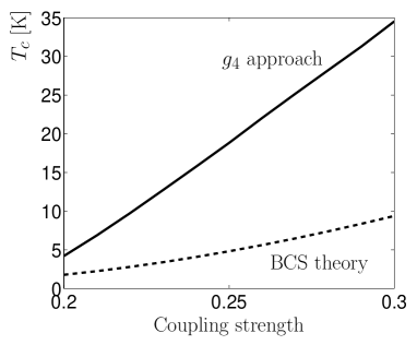
Figure 2: Transition temperature for the $g_{4}$ approach (upper curve) compared with the BCS result (lower curve) for $\hbar\omega_{D}=0.02$ eV. The effective dimensionless coupling strengths $g_{2}N_{0}$ and $g_{4}N_{0}^{2}\hbar\omega_{D}/4$ are assumed to be equal.

To solve the gap Eq. (24) of the four-fermion cluster, it is considered that the energies $\varepsilon_{{\bm{k}}_{1}}$ and $\varepsilon_{{\bm{k}}_{2}}$ are confined to a narrow interval around the Fermi surface so that the main contribution comes from ${\bm{q}}={\bm{0}}$. Adopting this approximation, we arrive at

$$\frac{g_{4}}{4}N_{0}^{2}\int\limits_{-\hbar\omega_{D}}^{\hbar\omega_{D}}dE_{1}dE_{2}\tanh\left(\frac{\beta_{c}E_{1}}{2}\right)\tanh\left(\frac{\beta_{c}E_{2}}{2}\right)\frac{\coth(\beta_{c}E_{1})+\coth(\beta_{c}E_{2})}{E_{1}+E_{2}}=1.$$ (27)

The numerical solution of this equation for characteristic coupling strengths of Cooperons is shown in Fig. 2 by the upper curve and compared with the BCS result (lower curve). For the comparison, the effective pair and four-body coupling constants were set to be equal. In this case, the transition temperature of four-fermion clusters is considerably higher than the BCS value. Whether the predicted high-transition temperature is realistic depends on possible values of the four-fermion coupling strength. The study of this problem requires further work that goes beyond the scope of our paper.

IV Summary

Guided by a Green function approach to BCS superconductivity, a superconducting phase transition has been identified in a fermionic system with a weakly attracting four-body interaction. The basic building blocks of the superconducting phase are quasi-particles that consist of four fermions hold together by an effective attraction. Special results have been obtained for the transition temperature $T_{c}$ by solving the gap equation. For comparable coupling strengths, the transition temperature of the four-fermion cluster model is much higher than the BCS values. This kind of superconductivity should be observable (preferentially by Andreev reflection) for strong coupling strengths within the four-fermion conglomerate. Whether the agglomerated attraction of four fermions can reach characteristic BCS values is a question that will decide future studies.

References

• (1) J. Bardeen, L. N. Cooper, and J. R. Schrieffer, Phys. Rev. 108, 1175 (1957).
• (2) J. Bardeen and D. Pines, Phys. Rev. 99, 1140 (1955).
• (3) J. G. Bednorz and K. A. Müller, Z. Phys. B64, 189 (1986).
• (4) R. J. Elliott, J. A. Krumhansl, and P. L. Leath, Rev. Mod. Phys. 46, 465 (1974).
• (5) M. Combescot and O. B. Matibet, Solid State Commun. 126, 687 (2003).
• (6) C. S. G. Cousins, J. Phys. F Metal Phys 3, 1915 (1973).
• (7) S. Ujevic and S. A. Vitiello, J. Phys.: Condens. Matter 19, 116212 (2007).
• (8) G. Date, P. K. Ghosh, and M. V. N. Murthy, Phys. Rev. Lett. 81, 3051 (1998).
• (9) C. Mora, A. Komnik, R. Egger, and A. O. Gogolin, Phys. Rev. Lett. 95, 080403 (2005).
• (10) L. P. Kadanoff and G. Baym, Quantum Statistical Mechanics (W. A. Benjamin, Inc., New York, 1962).
• (11) H. Puff, ZIE Preprint, 79-1, Berlin (in German) (1976).
• (12) P. Kleinert, phys. stat. sol. (b) 148, 325 (1988).