Stretching An Anisotropic DNA

Abstract

We present a perturbation theory to find the response of an anisotropic DNA to the external tension. It is shown that the anisotropy has a nonzero but small contribution to the force-extension curve of the DNA. Thus an anisotropic DNA behaves like an isotropic one with an effective bending constant equal to the harmonic average of its soft and hard bending constants.

1 Introduction

One of the most successful theories to describe the physical behavior of a long DNA molecule is the elastic rod model [1]. In this theory, the DNA is modeled as a continuous rod with intrinsic twist (to account for the helical structure of DNA) which changes its conformation in response to external forces or torques. The response of the DNA to an external stress is then mainly determined by three parameters: two principal bending constants and a twist constant. It is usually assumed that bending energy is isotropic.

Recent stretching experiments [2, 3, 4, 5] allow us to study mechanical response of a single DNA molecule. Marko and Siggia [6] reproduced the measured force-extension curve of DNA using the isotropic elastic rod model with an isotropic bending constant of about $50\,\mathrm{nm}$.

Because of DNA special structure, its bending energy is expected to be anisotropic. The existence of anisotropy in the bending of DNA has been previously reported by simulation studies as well [7, 8]. However, the exact values of the bending constants in the easy and hard directions (denoted here by $A_{1}$ and $A_{2}$, respectively) are still unknown. Recently, Olson et al. have stated that the ratio of the hard bending constant to the easy bending constant is in the range of $1$ to $5$ [9].

Since the isotropic elastic rod model can explain the observed force-extension curve in DNA stretching experiments, one may expect that the response of an anisotropic DNA to the external tension is similar to an isotropic DNA with an effective bending constant. For a free DNA the effective bending constant is given by [10]

$$\frac{1}{A_{\,eff}}=\frac{1}{2}(\frac{1}{A_{1}}+\frac{1}{A_{2}})\,.$$ (1)

We emphasize that the effective bending constant, in fact, depends on the external constrains applied to DNA. In case of a stretched DNA, the effective bending constant has been calculated by Nelson and Moroz [11] only at the large force limit. In this paper, we present a perturbation theory which allows us to calculate the force-extension curve of an anisotropic DNA, and find the effective bending constant.

2 The Model

2.1 The Elastic Rod Model

In the elastic rod model the DNA is represented by a continuous inextensible rod. The curve which passes through the rod center determines the configuration of the rod in three dimensional space. This curve is denoted by $\vec{r}$, and is parameterized by the arc length parameter $s$ (see Figure 1). In addition, a local coordinate system with axes $\{\hat{d_{1}},\hat{d_{2}},\hat{d_{3}}\}$ is attached to each point of the rod. $\hat{d_{3}}(s)$ is tangent to the curve $\vec{r}$ at each point

$$\hat{d_{3}}(s)=\frac{\mathrm{d}\vec{r}}{\mathrm{d}s}\,.$$ (2)

$\hat{d_{1}}(s)$ and $\hat{d_{2}}(s)$ lie in the plane of cross section of the DNA, and are chosen to be in the easy and hard directions of bending, respectively.

The orientation of the local coordinate system with respect to the laboratory coordinate system can be determined by an Euler rotation defined by

$$R(\alpha,\,\beta,\,\gamma)=R_{z}(\gamma)\,R_{y}(\beta)\,R_{z}(\alpha)\,.$$

$\alpha$, $\beta$, and $\gamma$ are Euler angles. The axes $\{\hat{d_{1}},\hat{d_{2}},\hat{d_{3}}\}$ can then be related to laboratory coordinate system, $\{\hat{x},\,\hat{y},\,\hat{z}\}$, via equations

$$\hat{d_{1}}=R^{\,-1}(\alpha,\,\beta,\,\gamma)\,\hat{x}\,,$$

$$\hat{d_{2}}=R^{\,-1}(\alpha,\,\beta,\,\gamma)\,\hat{y}\,,$$ (3)

$$\hat{d_{3}}=R^{\,-1}(\alpha,\,\beta,\,\gamma)\,\hat{z}\,.\,$$

Thus, if the Euler angles are known as a function of the arc length parameter $s$, the configuration of the rod will be uniquely determined.

From classical mechanics we know that

$$\dot{\hat{d_{i}}}=\vec{\Omega}\times\hat{d}_{i}\quad\quad\quad i=1,2,3\,.$$ (4)

where the dot denotes the derivative with respect to $s$, and $\Omega$ is called the spatial angular velocity. The components of $\vec{\Omega}$ in the local coordinate system are denoted by $\kappa_{1}$, $\kappa_{2}$, and $\omega$

$$\vec{\Omega}=\kappa_{1}\;\hat{d_{1}}+\kappa_{2}\;\hat{d_{2}}+\omega\;\hat{d_{3}}\,.$$ (5)

These components can be expressed in terms of Euler angles and their derivatives with respect to $s$ [12]

$$\kappa_{1}=\dot{\beta}\sin\gamma-\dot{\alpha}\sin\beta\cos\gamma\,\,,$$

$$\kappa_{2}=\dot{\beta}\cos\gamma+\dot{\alpha}\sin\beta\sin\gamma\,\,,$$ (6)

$$\omega=\dot{\gamma}+\dot{\alpha}\cos\beta\,.\qquad\qquad\quad$$

The elastic rod model introduces the elastic energy as a quadratic function of $\vec{\Omega}$ components [13]

$$E_{el}=\frac{1}{2}k_{B}T\int ds\,\Big{[}A_{1}\,\kappa_{1}^{2}+A_{2}\,\kappa_{2}^{2}+C\,(\omega-\omega_{0})^{2}\Big{]}\,$$ (7)

where $C$ is the twist constant, and $\omega_{0}$ is the intrinsic twist of DNA. the integral is over the entire length of the DNA. The first two terms in equation (7) correspond to the bending of DNA in the easy and hard directions, respectively. $A_{1}$ and $A_{2}$ are the corresponding bending constants $(A_{1}\leq A_{2})$. Note that the bending energy is isotropic for $A_{1}=A_{2}$. The third term indicates the energy needed for twisting the DNA about its central axis.

2.2 Partition Function of a Stretched DNA

In this section we present a standard method [6, 11, 12, 14] to calculate the statistical distribution function of the Euler angles, and to relate this distribution function to the partition function of a stretched DNA. We consider here the case of pure stretching, that is, stretching with zero applied torque. This situation is realized in many experiments [2, 3, 4, 5]. Also we assume all elastic modulus sequence independent and consider them to be constant.

Suppose that a DNA molecule is stretched by force $\vec{f}$ along $\mathbf{\mathrm{\hat{z}}}$ axis. Following [6, 11] we neglect self-avoidance effects. Thus the DNA in our model behaves like a phantom chain. we also neglect the electrostatic interactions, which are small if the salt concentration is high enough [2, 4, 5] . Then, total energy of DNA can be written as the sum of elastic energy and the potential energy associated with the tensile force

$$E_{tot}=E_{el}-fz\,,$$ (8)

where $z$ is the end-to-end extension of DNA in the direction of the external force and is given by

$$z=\int\hat{d_{3}}\cdot\mathbf{\mathrm{\hat{z}}}\,ds=\int\cos\beta\,ds\,.$$ (9)

Using equations (7) and (9), one can write

$$E_{tot}=\int e(s)\,ds\,,$$ (10)

where $e(s)$ is the energy per unit length of DNA and is given by

$$e(s)=k_{B}T\Big{[}\frac{1}{2}\,A_{1}\,\kappa_{1}^{2}+\frac{1}{2}\,A_{2}\,\kappa_{2}^{2}+\frac{1}{2}\,C\,(\omega-\omega_{0})^{2}-\tilde{f}\,\cos\beta\Big{]}\,,$$ (11)

where $\tilde{f}=\frac{f}{k_{B}T}$.

It is evident from equations (2.1) and (11) that the DNA total energy depends only on the Euler angles and their derivatives. This allows us to define a distribution function for Euler angles. For simplicity, we indicate the three Euler angles by the vector $\Theta=(\alpha,\,\beta,\,\gamma)$. In order to obtain the distribution function of $\Theta$, we first define the unnormalized Green function $\mathbf{G}(\Theta,\,s\,|\,\Theta_{0},\,0)$ as follows [12]

$$\mathbf{G}(\Theta_{f},\,s\,|\,\Theta_{0},\,0)=\int_{\Theta(0)=\Theta_{0}}^{\Theta(s)=\Theta_{f}}\!\mathcal{D}[\Theta]\exp\!\bigg{[}\!\!-\frac{1}{k_{B}T}\int_{0}^{s}e(s^{\prime})\,ds^{\prime}\bigg{]}.$$ (12)

The path integral in (12) is over all paths between $\Theta_{0}$ and $\Theta_{f}$. We define $\epsilon=\frac{s}{N+1}\,\,$, $\,s_{n}=n\,\epsilon$, and $\Theta_{n}=\Theta(s_{n})$. Then the path integral can be written as

$$\int_{\Theta(0)=\Theta_{0}}^{\Theta(s)=\Theta_{f}}\!\mathcal{D}[\Theta]=\!\!\!\!\!\!\!\!\lim_{\begin{subarray}{l}\\ \ \ \ \ \epsilon\longrightarrow 0\\ \\ \ \ \ \ N\longrightarrow\infty\\ \\ \ \ \ (N+1)\,\epsilon=s\end{subarray}}\!\!\!\!\!\Bigg{[}\mathcal{N}(\epsilon)\!\!\int d\Theta_{1}\int d\Theta_{2}\,\cdots\int d\Theta_{N}\Bigg{]}\,,$$ (13)

where $d\Theta_{n}=\sin\beta_{n}\,d\alpha_{n}\,\,d\beta_{n}\,\,d\gamma_{n}$  and

$$\mathcal{N}(\epsilon)=[\frac{A_{1}\,A_{2}\,C}{(2\pi\epsilon)^{\,3}}]^{\frac{N}{2}}\,.$$

We call $\mathbf{G}(\Theta,\,s\,|\,\Theta_{0},\,0)$ an unnormalized Green function since the condition $\int\mathbf{G}(\Theta,\,s\,|\,\Theta_{0},\,0)\,d\Theta=1$ is not satisfied for $f\neq 0$. The unnormalized Green function is in fact proportional to the distribution function of $\Theta$ at point $s$ for $\Theta(0)=\Theta_{0}$.
The above Green function satisfies a Schrodinger-like equation [12]

$$\left[\frac{\partial}{\partial s}+H\right]\!\mathbf{G}(\Theta,\,s\,|\,\Theta_{0},\,0)=\delta(s)\,\delta(\Theta-\Theta_{0})\,,$$ (14)

where the Hamiltonian $H$ is given by

$$H=\frac{J_{1}^{\,2}}{2A_{1}}+\frac{J_{2}^{\,2}}{2A_{2}}+\frac{J_{3}^{\,2}}{2C}+i\,\omega_{0}\,J_{3}-\tilde{f}\cos\beta\,,$$ (15)

with

$$J_{1}=-i\Big{[}-\frac{\cos\gamma}{\sin\beta}\,\frac{\partial}{\partial\alpha}+\sin\gamma\,\frac{\partial}{\partial\beta}+\cot\beta\,\cos\gamma\,\frac{\partial}{\partial\gamma}\Big{]}\,,$$

$$J_{2}=-i\Big{[}\quad\frac{\sin\gamma}{\sin\beta}\,\frac{\partial}{\partial\alpha}+\cos\gamma\,\frac{\partial}{\partial\beta}-\cot\beta\,\sin\gamma\,\frac{\partial}{\partial\gamma}\Big{]}\,,\,$$ (16)

$$J_{3}=-i\left[\frac{\partial}{\partial\gamma}\right].\qquad\qquad\qquad\qquad\qquad\qquad\qquad\ \quad\,\,$$

$J_{1}$, $J_{2}$, and $J_{3}$ are analogous to the angular momentum components of a quantum mechanical top with respect to a coordinate system attached to it. These angular momentum components satisfy the commutation relation [15]

$$[J_{i},J_{j}]=-i\,\epsilon_{ijk}\,J_{k}\,.$$ (17)

Note that the term $i\,\omega_{0}\,J_{3}$ makes the Hamiltonian non-Hermitian. In fact the Hamiltonian commutes with the time reversal operator and belongs to a class of Hamiltonians which are called pseudo-Hermitian [16].

The operators $J_{1}$ and $J_{2}$ can also be written in terms of ladder operators $J_{\pm}$

$$J_{1}=\frac{1}{2}(J_{+}+J_{-})\quad$$

$$J_{2}=\frac{1}{2i}(J_{+}-J_{-})\,.\,$$ (18)

Substituting $J_{1}$ and $J_{2}$ in equation (15) and using commutation relation (17), we obtain

$$H=\frac{1}{2A}J^{\,2}+(\frac{1}{2C}-\frac{1}{2A})J_{3}^{\,2}+\frac{1}{4}\frac{\lambda}{A}(J_{+}^{\,2}+J_{-}^{\,2})+i\,\omega_{0}\,J_{3}-\tilde{f}\cos\beta\,,$$ (19)

here $A$ is the harmonic average of $A_{1}$ and $A_{2}$

$$\frac{1}{A}=\frac{1}{2}(\frac{1}{A_{1}}+\frac{1}{A_{2}})\,,$$ (20)

and

$$\lambda=\frac{A_{2}-A_{1}}{A_{1}+A_{2}}\,.$$ (21)

$\lambda$ is a dimensionless parameter characterizing the anisotropy and varies between zero and one.

We denote the distribution function of $\Theta$ at the point $s$ by $\Psi(\Theta,s)$. From the definition of Green function it is obvious that $\Psi(\Theta,\,s)$ can be related to $\Psi(\Theta,\,0)$ via equation

$$\Psi(\Theta,\,s)=\int G(\Theta,\,s|\Theta_{0},\,0)\,\Psi(\Theta_{0},\,0)\,d\Theta_{0}\,.$$ (22)

Notice that since the Green function is not normalized, $\Psi(\Theta,s)$ is not normalized either, so we refer to it as the unnormalized distribution function. Considering (22), $\Psi(\Theta,s)$ also satisfies equation (14)

$$H\,\Psi(\Theta,s)=-\frac{\partial}{\partial s}\Psi(\Theta,s)\qquad s>0\,.$$ (23)

Therefore, we can find $\Psi(\Theta,s)$ by solving the above Schrodinger-like equation.
We now use Dirac notation to present our results in a more familiar form. Replacing $\Psi(\Theta,s)$ with $\langle\Theta\,|\Psi(s)\rangle$ we can rewrite equation (23) as

$$H\,|\Psi(s)\rangle=-\frac{\partial}{\partial s}|\Psi(s)\rangle\,.$$ (24)

Using equations (12), (13), and (22), the partition function of a stretched DNA can be written as [14]

$$Z=\int\langle\Theta|\Psi(L)\rangle\,d\Theta\,,$$ (25)

where $L$ is the total length of DNA. Hence, in order to find the partition function one must solve the Schrodinger-like differential equation (23) and integrate the solution over all $\Theta$ values.

To solve equation (23), we rewrite the Hamiltonian in the form

$$H=H_{0}+\lambda\,V\,,$$ (26)

where

$$H_{0}=\frac{1}{2A}J^{\,2}+(\frac{1}{2C}-\frac{1}{2A})J_{3}^{\,2}+i\,\omega_{0}\,J_{3}-\tilde{f}\cos\beta\,,$$ (27)

and

$$V=\frac{1}{4\,A}(J_{+}^{2}+J_{-}^{2})\,.$$ (28)

Furthermore, we decompose $H_{0}$ to its real and imaginary parts

$$H_{0}=H_{0}^{R}+iH_{0}^{I}\,,$$ (29)

where

$$H_{0}^{R}=\frac{J^{2}}{2\,A}+(\frac{1}{2\,C}-\frac{1}{2\,A})\,J_{3}^{2}-\tilde{f}\,\cos\beta$$ (30)

and

$$H_{0}^{I}=\omega_{0}\,J_{3}\,.$$ (31)

$H_{0}^{\,R}$ is the Hamiltonian of a quantum top. It commutes with both $J_{3}$ and $J_{z}$, where $J_{z}$ is the third component of the angular momentum operator in the laboratory coordinate system [15]. Since $J_{3}$ and $J_{z}$ also commute with each other, one can find the simultaneous eigenvectors of these three operators. We denote these simultaneous eigenvectors by $|n,\,k,\,m\rangle$ where $k$ and $m$ are integer numbers referring to the eigenvalues of $J_{3}$ and $J_{z}$, respectively. The quantum number $n$ distinguishes between the eigenvectors with identical $k$ and $m$ numbers:

$$H_{0}^{R}\,\,|n,k,m\rangle=\mathcal{E}_{n,\,k,\,m}^{\,R}\,\,|n,k,m\rangle\,,$$ (32)

$$J_{3}\,|n,k,m\rangle=k\,|n,k,m\rangle\,,\qquad\quad$$ (33)

$$J_{z}\,|n,k,m\rangle=m\,|n,k,m\rangle\,.\qquad\quad$$ (34)

From equations (27), (32), and (33), it can further be seen that the eigenvectors of $H_{0}^{\,R}$ are also eigenvectors of $H_{0}$:

$$H_{0}\,\,|n,k,m\rangle=\mathcal{E}_{n,\,k,\,m}^{\,0}\,\,|n,k,m\rangle\,,$$ (35)

where

$$\mathcal{E}_{n,\,k,\,m}^{\,0}=\mathcal{E}_{n,\,k,\,m}^{\,R}+i\,k\,\omega_{0}\,.$$ (36)

Since $H_{0}^{\,R}$ is Hermitian, its eigenvectors form a complete orthogonal basis [17]. We now expand $|\Psi(s)\rangle$ in terms of $|n,\,k,\,m\rangle$ eigenvalues

$$|\Psi(s)\rangle=\sum_{n,k,m}C_{n,\,k,\,m}(s)\,\,\mathrm{e}^{-\mathcal{E}_{n,\,k,\,m}^{\,0}\,s}\,|n,k,m\rangle$$ (37)

and substitute $|\Psi(s)\rangle$ into equation (24). Taking the orthogonality of the eigenvectors into account we obtain

$$\frac{\partial}{\partial s}\,C_{n,\,k,\,m}=-\lambda\!\!\sum_{n^{\prime},k^{\prime},m^{\prime}}\langle n,k,m|V|n^{\prime},k^{\prime},m^{\prime}\rangle\mathrm{e}^{-(\,\mathcal{E}_{n^{\prime},\,k^{\prime},\,m^{\prime}}^{\,0}-\mathcal{E}_{n,\,k,\,m}^{\,0})\,s\,}\,C_{n^{\prime},\,k^{\prime},\,m^{\prime}}\,.\quad$$ (38)

The ladder operators in $V$ imply that [15]

$$\langle n,k,m|V|n^{\prime},k^{\prime},m^{\prime}\rangle=\langle n,k,m|V|n^{\prime},k+2,m\rangle\,\delta_{m^{\prime},m}\,\delta_{k^{\prime},k+2}+$$

$$\langle n,k,m|V|n^{\prime},k-2,m\rangle\,\delta_{m^{\prime},m}\,\delta_{k^{\prime},k-2}\,.\$$ (39)

so we have

$$\frac{\partial}{\partial s}\,C_{n,\,k,\,m}=-\lambda\,\sum_{n^{\prime}}\langle n,k,m|V|n^{\prime},k+2,m\rangle\mathrm{e}^{-(\,\mathcal{E}_{n^{\prime},\,k+2,\,m}^{\,0}-\mathcal{E}_{n,\,k,\,m}^{\,0})\,s\,}\,C_{n^{\prime},\,k+2,\,m}$$

$$-\lambda\,\sum_{n^{\prime}}\langle n,k,m|V|n^{\prime},k-2,m\rangle\mathrm{e}^{-(\mathcal{E}_{n^{\prime},\,k-2,\,m}^{\,0}-\mathcal{E}_{n,\,k,\,m}^{\,0})\,s}\,C_{n^{\prime},\,k-2,\,m}\,.$$ (40)

Substituting $|\psi(L)\rangle$ from equation (37) into equation (25) we can derive an expression for the partition function. Since $\int\langle\Theta|n,\,k,\,m\rangle\,d\Theta$ is non-zero only for $k=m=0$, we obtain [15]

$$Z=\sum_{n}I_{n}\,C_{n,0,0}(L)\,e^{-\mathcal{E}_{n,\,0,\,0}^{\,0}\,L}$$ (41)

where

$$I_{n}\equiv\int\langle\Theta|n,\,0,\,0\rangle\,d\Theta\,.$$ (42)

Thus, to determine the partition function of a stretched DNA, one needs to find the coefficients $C_{n,0,0}(L)$ by solving the differential equation (2.2).

2.3 Perturbation Theory

In this section, we use perturbation theory to find the expansion coefficients and the partition function in powers of $\lambda$. Let’s expand $C_{n,k,m}(s)$ in terms of $\lambda$:

$$C_{n,k,m}(s)=\sum_{p=0}^{\infty}{\lambda}^{p}\,C^{\,(p)}_{n,k,m}(s)\,.$$ (43)

As a result, the partition function can be written as

$$Z=\sum_{p=0}^{\infty}\lambda^{p}\,Z^{\,(p)}\,,$$ (44)

where

$$Z^{\,(p)}=\sum_{n}I_{n}\,C^{\,(p)}_{n,0,0}(L)\,e^{-\mathcal{E}_{n,\,0,\,0}^{\,0}\,L}\,.$$ (45)

By inserting $C_{n,k,m}(s)$ from equation (43) into equation (2.2), one can see that $C^{\,(p)}_{n,0,0}(s)$ satisfies the following differential equations

$$\frac{\partial}{\partial s}\,C^{\,(0)}_{n,\,k,\,m}=0$$ (46)

for $p=0$, and

$$\frac{\partial}{\partial s}\,C^{\,(p)}_{n,\,k,\,m}=-\sum_{n^{\prime}}\langle n,k,m|V|n^{\prime},k+2,m\rangle\mathrm{e}^{-(\,\mathcal{E}_{n^{\prime},\,k+2,\,m}^{\,0}-\mathcal{E}_{n,\,k,\,m}^{\,0})\,s\,}\,C^{\,(p-1)}_{n^{\prime},\,k+2,\,m}$$

$$-\sum_{n^{\prime}}\langle n,k,m|V|n^{\prime},k-2,m\rangle\mathrm{e}^{-(\mathcal{E}_{n^{\prime},\,k-2,\,m}^{\,0}-\mathcal{E}_{n,\,k,\,m}^{\,0})\,s}\,C^{\,(p-1)}_{n^{\prime},\,k-2,\,m}\quad\quad$$ (47)

for $p>0$.
The value of $|\Psi(0)\rangle$ is determined by anchoring the DNA hence independent of $\lambda$. Thus the corresponding initial conditions are

$$C^{\,(0)}_{n,k,m}(0)=C_{n,k,m}(0)\ \quad\,\textrm{for}\ p=0\,\,$$

$$C^{\,(p)}_{n,k,m}(0)=0\quad\textrm{for}\ p>0\,.\qquad\qquad$$ (48)

It can be seen from equation (46) that $C^{\,(0)}_{n,\,k,\,m}$ is constant

$$C^{\,(0)}_{n,k,m}=C_{n,k,m}(0)\,.$$ (49)

Therefore, the partition function to the zeroth order of $\lambda$ is given by

$$Z^{\,(0)}=\sum_{n,k}b^{\,(0)}_{n,k}\,\,e^{-\mathcal{E}_{n,\,k,\,0}^{\,0}\,L}\,,$$ (50)

where

$$b^{\,(0)}_{n,k}=I_{n}\,C^{\,(0)}_{n,0,0}\,\,\delta_{k,0}\,.$$ (51)

$Z^{(\,0)}$ is the partition function of an isotropic DNA with bending constant $A$.
The differential equation (2.3) can be solved by iteration, and the corrections to $Z^{(\,0)}$ can be found in powers of $\lambda$. The first order correction is given by

$$Z^{\,(1)}=\sum_{n,k}b^{\,(1)}_{n,k}\,\,e^{-\mathcal{E}_{n,\,k,\,0}^{\,0}\,L}\,,$$ (52)

and the second order correction is given by

$$Z^{\,(2)}=\sum_{n,k}(b^{\,(2)}_{n,k}-U^{\,(2)}_{n}\,C^{\,(0)}_{n,0,0}\,\delta_{k,0}\,L)\,\,e^{-\mathcal{E}_{n,\,k,\,0}^{\,0}\,L}\,.$$ (53)

The coefficients $b^{\,(1)}_{n,k}$ and $b^{\,(2)}_{n,k}$ in equations (52) and (53) are given in appendix A. They depend on the initial conditions but do not depend on the length of DNA. The coefficient $U^{\,(2)}_{n}$ is given by

$$U^{\,(2)}_{n}=\sum_{n_{1}\notin G_{n},\,n_{2}}I_{n_{1}}\bigg{[}\frac{\langle n_{1},\,0|V|n_{2},\,2\rangle\,\langle n_{2},\,2|V|n,\,0\rangle}{(\mathcal{E}_{n,\,0}^{\,0}-\mathcal{E}_{n_{2},\,2}^{\,0})}+$$

$$\frac{\langle n_{1},\,0|V|n_{2},\,-2\rangle\,\langle n_{2},\,-2|V|n,\,0\rangle}{(\mathcal{E}_{n,\,0}^{\,0}-\mathcal{E}_{n_{2},\,-2}^{\,0})}\bigg{]},$$ (54)

where for simplicity, we omit the quantum number $m$ keeping in mind that $m=0$. $G_{n}$ in equation (2.3) refers to all eigenvectors with eigenvalues equal to $\mathcal{E}_{n,\,0,\,0}^{\,0}$

$$n_{1}\in G_{n}\Leftrightarrow\mathcal{E}_{n_{1},\,0,\,0}^{\,0}=\mathcal{E}_{n,\,0,\,0}^{\,0}\,.$$ (55)

Clearly, if the eigenvector $|n,\,0,\,0\rangle$ is not degenerate, we have $G_{n}=\{n\}$.

The coefficients $b^{\,(1)}_{n,k}$ are zero except for $k=0,\pm 2$ (see appendix A). Since the imaginary part $\mathcal{E}_{n,\,k,\,0}^{\,0}$ is $k\,\omega_{0}$, an oscillatory term with frequency $2\,\omega_{0}$ appears in $Z^{(\,1)}$. In fact, from equation (2.3) we expect that oscillatory terms with frequencies $\{2\,\omega_{0},\,4\,\omega_{0},\,\cdots\,,2p\,\omega_{0}\}$ appear in the expression of $Z^{(\,p)}$. The appearance of oscillatory terms is, in fact, an artifact of coupling between bending and twisting in an anisotropic DNA [18]. This is the main difference between the partition functions of an isotropic and an anisotropic DNA. Although, as we will show in the next section, this difference is not detectable in experiments, at least if the DNA is long enough.

2.4 The Average End to End Extension

Using equations (8), (12), (22), and (25) the average end-to-end extension of the DNA can be calculated as [6, 11]

$$\frac{\langle z\rangle}{L}=\frac{1}{L}\,\frac{\partial\ln Z}{\partial\tilde{f}}\,.$$ (56)

Following Marko and Siggia [6], we limit our study to the long DNA. In this case, because of the presence of $\exp(-\mathcal{E}_{n,\,k,\,0}^{\,R}\,L)$ factor, the term which corresponds to the ground state eigenvalue of $H_{0}^{\,R}$ is much greater than other terms in the expansion of the partition function. Therefore, the partition function can be approximated only by the ground state term where all other terms can be neglected. If we denote the difference between the ground state and the first excited state eigenvalues by $\Delta\mathcal{E}^{R}$ then the long DNA limit corresponds to the condition $\Delta\mathcal{E}^{R}L\gg 1$. We will discuss in the next section that this condition is indeed satisfied in the stretching experiments.

The operator $H_{0}^{\,R}$ is the Hamiltonian of a top in a uniform external field, and its ground state is unique. Thus the ground state of $H_{0}^{\,R}$ must be a simultaneous eigenvector of $J_{3}$ and $J_{z}$, with eigenvalues $m=k=0$ [6]. We denote the ground state and its eigenvalue by $|0,0,0\rangle$ and $\mathcal{E}_{0,\,0,\,0}^{\,R}$ respectively. Therefore, at long DNA limit we obtain

$$Z^{\,(0)}\simeq b^{\,(0)}_{0,0}\,\,e^{-\mathcal{E}_{0,\,0,\,0}^{\,0}\,L}\,,$$ (57)

$$Z^{\,(1)}\simeq b^{\,(1)}_{0,0}\,\,e^{-\mathcal{E}_{0,\,0,\,0}^{\,0}\,L}\,,$$ (58)

and

$$Z^{\,(2)}\simeq(b^{\,(2)}_{0,0}-U^{\,(2)}_{0}\,C^{\,(0)}_{0,0,0}\,L)\,\,e^{-\mathcal{E}_{0,\,0,\,0}^{\,0}\,L}\,.$$ (59)

Since the ground state is not degenerate, $G_{0}=\{0\}$ and one can write

$$U_{0}^{\,(2)}=\mathcal{E}_{0,\,0,\,0}^{\,2}\,I_{0}\,,$$ (60)

where

$$\mathcal{E}^{\,2}_{0,0,0}=\sum_{n_{2}}\bigg{[}\,\frac{\big{|}\langle 0,\,0,\,0|\,V|n_{2},\,2,\,0\rangle\big{|}^{\,2}}{(\mathcal{E}_{0,\,0,\,0}^{\,0}-\mathcal{E}_{n_{2},\,2,\,0}^{\,0})}+\frac{\big{|}\langle 0,\,0,\,0|\,V|n_{2},\,-2,\,0\rangle\big{|}^{\,2}}{(\mathcal{E}_{0,\,0,\,0}^{\,0}-\mathcal{E}_{n_{2},\,-2,\,0}^{\,0})}\,\bigg{]}.$$ (61)

Therefore, $Z^{\,(2)}$ can be written as

$$Z^{\,(2)}\simeq(b^{\,(2)}_{0,0}-b^{\,(0)}_{0,0}\,\mathcal{E}^{\,2}_{0,0,0}\,L)\,\,e^{-\mathcal{E}_{0,\,0,\,0}^{\,0}\,L}\,.$$ (62)

We expand $\langle z\rangle$ in powers of $\lambda$,

$$\frac{\langle z\rangle}{L}=\frac{\langle z^{\,(0)}\rangle}{L}+\lambda\frac{\langle z^{\,(1)}\rangle}{L}+\lambda^{2}\frac{\langle z^{\,(2)}\rangle}{L}+O(\lambda^{3})\,.$$ (63)

From equation (56), we have

$$\frac{\langle z^{\,(0)}\rangle}{L}=\frac{1}{L}\,\frac{\partial\ln Z^{\,(0)}}{\partial\tilde{f}}\,,$$ (64)

$$\frac{\langle z^{\,(1)}\rangle}{L}=\frac{1}{L}\,\frac{\partial}{\partial\tilde{f}}\,\frac{\partial\ln Z}{\partial\lambda}\bigg{|}_{\lambda=0}=\frac{1}{L}\,\frac{\partial}{\partial\tilde{f}}\,\frac{Z^{\,(1)}}{Z^{\,(0)}}\,,\!\!\!\!\quad\quad\qquad\,\,$$ (65)

and

$$\frac{\langle z^{\,(2)}\rangle}{L}=\frac{1}{2\,L}\,\frac{\partial}{\partial\tilde{f}}\,\frac{\partial^{2}\ln Z}{\partial\lambda^{2}}\bigg{|}_{\lambda=0}=\frac{1}{L}\,\frac{\partial}{\partial\tilde{f}}\,\bigg{[}\frac{Z^{\,(2)}}{Z^{\,(0)}}-\frac{1}{2}\Big{(}\frac{Z^{\,(1)}}{Z^{\,(0)}}\Big{)}^{2}\bigg{]}\,.$$ (66)

Neglecting terms of order $\frac{1}{L}$ [6, 11], we obtain

$$\frac{\langle z^{\,(0)}\rangle}{L}\simeq-\frac{\partial\mathcal{E}^{\,0}_{0,0,0}}{\partial\tilde{f}}\,,$$ (67)

$$\frac{\langle z^{\,(1)}\rangle}{L}\approx 0\,,\ \qquad\,\,$$ (68)

$$\frac{\langle z^{\,(2)}\rangle}{L}\simeq-\frac{\partial\mathcal{E}^{\,2}_{0,0,0}}{\partial\tilde{f}}\,.$$ (69)

So far we have assumed that DNA is inextensible. To account for the extensibility of DNA the term $\frac{\tilde{f}}{B}$ must be added to $\frac{\langle z\rangle}{L}$ , where $B\,k_{B}T$ is the stretch modulus of DNA and is about $500\,\mathrm{k_{B}T\,nm^{-1}}$ [6]. Thus one can write

$$\frac{\langle z^{\,(0)}\rangle}{L}\simeq-\frac{\partial\mathcal{E}^{\,0}_{0,0,0}}{\partial\tilde{f}}+\frac{\tilde{f}}{B}\,.$$ (70)

$\langle z^{\,(0)}\rangle$ is the average end-to-end extension of an isotropic DNA with the bending constant $A$. Marko and Siggia have also calculated $\langle z^{\,(0)}\rangle$ [6]. Although they used a different Hamiltonian, i.e.

$$H_{iso}=\frac{J^{2}}{2\,A}-\tilde{f}\cos\beta\,,$$

our results are identical to theirs to the zeroth order. The reason is that $H_{0}^{\,R}$ and $H_{iso}$ have the same ground state eigenvalues.

3 Results

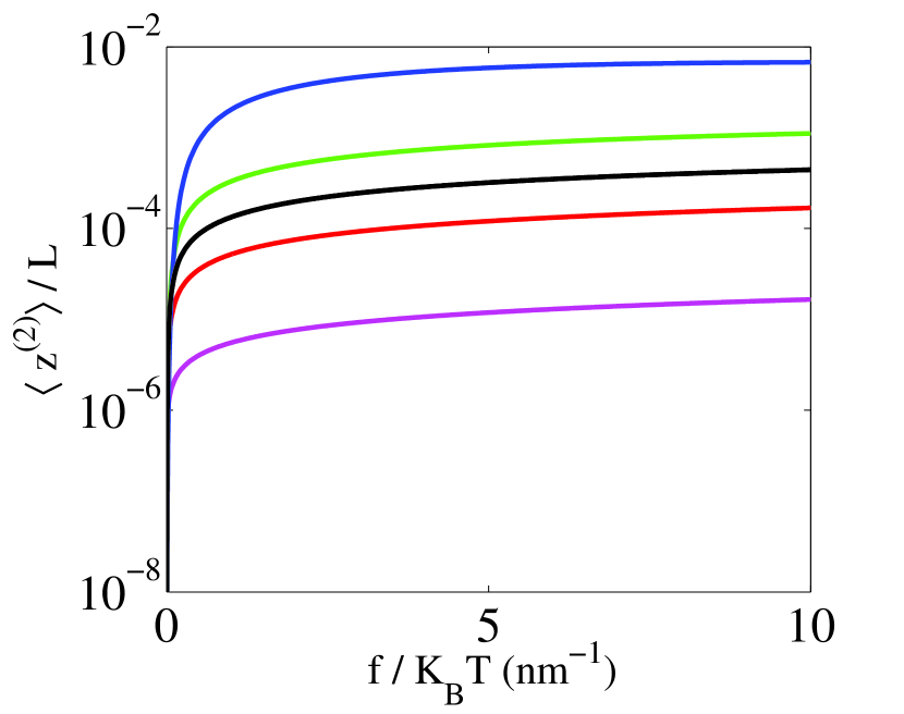
Numerical methods are employed (see appendix B) to calculate the second order correction to the force extension curve of an isotropic DNA, assuming $A=50\,\mathrm{nm}$, $C=100\,\mathrm{nm}$ [11], and $\omega_{0}=1.8\,\mathrm{nm^{-1}}$. The result is shown in Figure 2. For forces slightly greater than $\tilde{f}\sim 10\,\mathrm{nm^{-1}}$ the DNA undergoes an over-stretching transition [19], hence the elastic rod model is not relevant. We have therefore picked the force range of $0<\tilde{f}<10\,\mathrm{nm^{-1}}$ to insure validity.

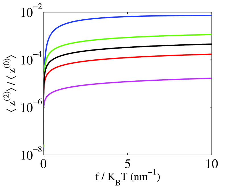
It can be seen from Figure 2 that $\langle z^{\,(2)}\rangle$ is positive. Therefore, to the second order of $\lambda$, anisotropy increases the average extension of DNA. However, $\langle z^{\,(2)}\rangle$ is small compared to $\langle z^{\,(0)}\rangle$. For $A=50\,\mathrm{nm}$, the maximum value of the ratio $\frac{\langle z^{\,(2)}\rangle}{\langle z^{\,(0)}\rangle}$ is in the order of $10^{-4}$ (see Figure 3).
To be sure that this result is not limited to the special case of $A=50\,\mathrm{nm}$, we examine four different values of $A$ in the range $5\leq A\leq 500\,\mathrm{nm}$ (see Figure 2). The ratio $\frac{\langle z^{\,(2)}\rangle}{\langle z^{\,(0)}\rangle}$ for these four values of $A$ are plotted in Figure 3. It can be seen that $\frac{\langle z^{\,(2)}\rangle}{\langle z^{\,(0)}\rangle}$ does not exceed $10^{-2}$ for $A\geq 5\mathrm{nm}$.

As can be seen from Figure 2, for $A=50\,\mathrm{nm}$, where the theoretical curve is best fitted to the experimental data [6], one must measure $\frac{\langle z\rangle}{L}$ at least with the accuracy $10^{-4}$ to detect $\langle z^{\,(2)}\rangle$ . Since $L\sim 10\,\mathrm{\mu m}$ in experiments [2], minimum accuracy of $1\,\mathrm{nm}$ is required in measuring $\langle z\rangle$. However, the accuracy of the experiments is by far less than this limit [2], therefore $\langle z^{\,(2)}\rangle$ can not be detected by stretching experiments.

We now show that $\langle z^{\,(3)}\rangle$ is also small. It is obvious that when $\Psi(\Theta,0)$ is independent of the Euler angle $\gamma$, the partition function is invariant under the transformation $\lambda\rightarrow-\lambda$. This means that odd powers of $\lambda$ are not present in the expansion of $\langle z\rangle$, i.e., $\langle z^{\,(2p+1)}\rangle=0$. In addition, the effect of the initial conditions on the force extension curve of DNA is suppressed if DNA is long enough. As a result, one expects $\frac{\langle z^{\,(2p+1)}\rangle}{L}$ to be small even when $\Psi(\Theta,0)$ depends on $\gamma$. In other words, odd powers of $\lambda$ have no significant contribution to the end-to-end DNA extension. Therefore, to the third order of $\lambda$, the response of an anisotropic DNA to the external tension is close to an isotropic DNA with the effective bending constant

$$A_{eff}=A=2\left(\frac{1}{A_{1}}+\frac{1}{A_{2}}\right)^{-1}\,.$$ (71)

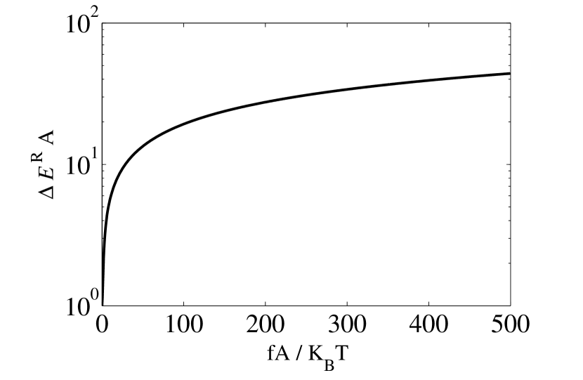
To justify our result, we must show that the condition $\Delta\mathcal{E}^{R}L\gg 1$ which corresponds to the limit of long DNA, is satisfied in experiments as well. Figure 4 shows $\Delta\mathcal{E}^{R}A$ as a function of $\tilde{f}A$ for $A=50\,\mathrm{nm}$. As can be seen, $\Delta\mathcal{E}^{R}A\geq 1$. As a result, the condition $\Delta\mathcal{E}^{R}L\gg 1$ is equivalent to the condition $L\gg A$, which is well known in polymer physics. Since $A=50\,\mathrm{nm}$ and $L\sim 10\,\mathrm{\mu m}$, this condition is satisfied in the streching experiments.

4 Discussion and Conclusion

It is well known that when DNA is free (i.e., no external force applied), the average energy of an anisotropic DNA is equal to the average energy of an isotropic DNA with bending constant $A$ [8]. Moreover, Maddocks and Kehrbaum [10] have proved that in the absence of external forces or torques the ground state configuration of an anisotropic DNA is similar to the ground state configuration of an isotropic DNA with bending constant $A$. However, a stretched DNA is not free. More importantly, to calculate the average end-to-end extension one must deal with the free energy instead of the average energy or the ground state energy.

The partition function of a stretched DNA is generally represented as

$$Z=\int_{E_{min}}^{\infty}\mathcal{D}(E)\,\exp(-\frac{E}{k_{B}T})\,\mathrm{d}E\,,$$ (72)

where $\mathcal{D}(E)\,\mathrm{d}E$ is the number of possible configuration with an energy in the range of $E$ and $E+\mathrm{d}E$, and $E_{min}$ is the ground state energy. For an stretched DNA, the ground state corresponds to the configuration in which the DNA is fully stretched. The equilibrium configuration of the DNA is the configuration that minimize the free energy, $F=E-k_{B}T\ln\mathcal{D}(E)$, and therefore is different from the ground state configuration. Clearly, bending anisotropy changes $\mathcal{D}(E)$ for excited configurations thus changes the free energy and equilibrium configuration of the stretched DNA. When no external force is applied to the DNA, the number of configurations that have the end-to-end extension $z$ is exactly equal to the number of configurations with the end-to-end extension $-z$. Consequently we have $\langle z\rangle=0$ regardless of the degree of anisotropy, $\lambda$. Thus in the limit of $\tilde{f}A\ll 1$, anisotropy can barely affect the average end-to-end extension, and one expects $\langle z^{\,(2)}\rangle$ and in fact all the higher-order corrections to be small, as can be seen from Figures 2 and 3. On the other hand, in the limit of $\tilde{f}A\gg 1$, the energy of the ground state is much lower than those of the excited states, and the excited configurations have a small contribution to the partition function. Therefore, the effect of anisotropy will be suppressed at large forces, and $\langle z^{\,(2)}\rangle$ and all the higher-order corrections vanish as $\tilde{f}A\rightarrow\infty$. This is the reason that $\frac{\partial\langle z^{\,(2)}\rangle}{\partial f}$ is smaller at large forces (see Figure 2).

Nelson and Moroz [11] have applied an approximate method to obtain an analytical expression for $\langle z\rangle$ at the limit of large forces to the second order of $\lambda$. They found

$$A_{eff}=\bar{A}(1-2(\frac{\hat{A}}{\stackrel{{\scriptstyle}}{{\bar{A}}}})^{2})=A-\lambda^{2}\,\bar{A}\,,$$

with $\bar{A}=\frac{1}{2}(A_{1}+A_{2})$, and $\hat{A}=\frac{1}{2}(A_{2}-A_{1})$. This result is different from equation (71). However, we rederived their calculations and obtained the same result as in equation (71)

$$A_{eff}=\bar{A}(1-(\frac{\hat{A}}{\stackrel{{\scriptstyle}}{{\bar{A}}}})^{2})=A$$

Thus we believe that they just made an error in their calculations. It can be shown that the result of these calculations is in fact exact (see appendix C). Therefore, at the high force limit, an anisotropic DNA behaves like an isotropic DNA with the bending constant $A$.

5 Acknowledgement

We thank N. Hamedani Radja for insightful conversations and his valuable comments on analytical calculations. We do also thank H. Amirkhani for her comments on the draft manuscript and Behzad Eslami-Mossallam for the figures illustrations. MRE thanks the Center of Excellence in Complex Systems and Condensed Matter (CSCM) and the Institute for studies in Theoretical Physics and Mathematics for their partial supports.

Appendix A Expansion Coefficients for $Z^{\,(1)}$ and $Z^{\,(2)}$

Here we present the expressions for $b^{\,(1)}_{n,k}$ and $b^{\,(2)}_{n,k}$. Let’s use the following abbreviations

$$V_{n,\,k,\,n^{\prime},\,k^{\prime}}\equiv\langle n,\,k,\,0|\,V|n^{\prime},\,k^{\prime},\,0\rangle\,,$$ (73)

and

$$\Delta\mathcal{E}_{n,\,k,\,n^{\prime},\,k^{\prime}}^{\,0}=\mathcal{E}_{n,\,k,\,0}^{\,0}-\mathcal{E}_{n^{\prime},\,k^{\prime},\,0}^{\,0}\,.$$ (74)

The $b^{\,(1)}_{n,k}$ coefficients are

$$b^{\,(1)}_{n,\pm 2}=\sum_{n_{1}}I_{n_{1}}\,\frac{V_{n_{1},\,0,\,n,\,\pm 2}}{\Delta\mathcal{E}_{n,\,\pm 2,\,n_{1},\,0}^{\,0}}\,\,C_{n_{1},\pm 2,0}^{(0)},\qquad\qquad\qquad\quad\quad\quad$$ (75)

$$b^{\,(1)}_{n,0}=I_{n}\,\sum_{n_{1}}\,\Big{[}\frac{V_{n,\,0,\,n_{1},\,2}}{\Delta\mathcal{E}_{n,\,0,\,n_{1},\,2}^{\,0}}\,\,C_{n_{1},2,0}^{(0)}+\frac{V_{n,\,0,\,n_{1},\,-2}}{\Delta\mathcal{E}_{n,\,0,\,n_{1},\,-2}^{\,0}}\,\,C_{n_{1},-2,0}^{(0)}\Big{]},$$ (76)

and

$$b^{\,(1)}_{n,k}=0\qquad k\neq 0,\,\pm 2\,.\qquad\qquad\qquad\qquad\qquad\qquad\qquad\quad\,\,\,\,$$ (77)

The $b^{\,(2)}_{n,k}$ coefficients are

$$b^{\,(2)}_{n,\pm 4}=\sum_{n_{1},n_{2}}I_{n_{1}}\Big{[}\frac{V_{n_{1},\,0,\,n_{2},\,\pm 2}\,\,V_{n_{2},\,\pm 2,\,n,\,\pm 4}}{\Delta\mathcal{E}_{n,\,\pm 4,\,n_{1},\,0}^{\,0}\,\,\Delta\mathcal{E}_{n,\,\pm 4,\,n_{2},\,\pm 2}^{\,0}}\Big{]}C_{n,\pm 4,0}^{(0)},$$ (78)

$$b^{\,(2)}_{n,\pm 2}=\sum_{n_{1},n_{2}}I_{n_{2}}\Big{[}\frac{V_{n_{2},\,0,\,n,\,\pm 2}\,\,V_{n,\,\pm 2,\,n_{1},\,\pm 4}}{\Delta\mathcal{E}_{n,\,\pm 2,\,n_{1},\,\pm 4}^{\,0}\,\,\Delta\mathcal{E}_{n,\,\pm 2,\,n_{2},\,0}^{\,0}}\,\,C_{n_{1},\pm 4,0}^{(0)}$$

$$+\frac{V_{n_{2},\,0,\,n,\,\pm 2}\,\,V_{n,\,\pm 2,\,n_{1},\,0}}{\Delta\mathcal{E}_{n,\,\pm 2,\,n_{1},\,0}^{\,0}\,\,\Delta\mathcal{E}_{n,\,\pm 2,\,n_{2},\,0}^{\,0}}\,\,C_{n_{1},0,0}^{(0)}\Big{]},$$ (79)

$$b^{\,(2)}_{n,0}=\sum_{n_{1},\,n_{2}}\sum_{k=\pm 2}I_{n}\Big{[}\frac{V_{n,\,0,\,n_{2},\,k}\,\,V_{n,\,k,\,n_{1},\,2k}}{\Delta\mathcal{E}_{n_{1},\,2k,\,n_{2},\,k}^{\,0}\,\,\Delta\mathcal{E}_{n,\,0,\,n_{1},\,2k}^{\,0}}\qquad\quad$$

$$-\frac{V_{n,\,0,\,n_{2},\,k}\,\,V_{n,\,k,\,n_{1},\,2k}}{\Delta\mathcal{E}_{n_{1},\,2k,\,n_{2},\,k}^{\,0}\,\,\Delta\mathcal{E}_{n,\,0,\,n_{2},\,k}^{\,0}}\Big{]}C_{n_{1},2k,0}^{(0)}$$

$$-\sum_{n_{1},\,n_{2}}\sum_{k=\pm 2}I_{n}\Big{[}\frac{V_{n,\,0,\,n_{2},\,k}\,\,V_{n_{2},\,k,\,n_{1},\,0}}{\Delta\mathcal{E}_{n,\,0,\,n_{2},\,k}^{\,0}\,\,\Delta\mathcal{E}_{n_{1},\,0,\,n_{2},\,k}^{\,0}}\Big{]}C_{n_{1},0,0}^{(0)}$$

$$+\sum_{\begin{subarray}{l}n_{1},\,n_{2}\\ n_{1}\notin G_{n}\end{subarray}}\sum_{k=\pm 2}I_{n_{1}}\Big{[}\frac{V_{n_{1},\,0,\,n_{2},\,k}\,\,V_{n_{2},\,k,\,n,\,0}}{\Delta\mathcal{E}_{n,\,0,\,n_{2},\,k}^{\,0}\,\,\Delta\mathcal{E}_{n,\,0,\,n_{1},\,0}^{\,0}}\Big{]}C_{n,0,0}^{(0)}$$

$$-\sum_{\begin{subarray}{l}n_{1},\,n_{2}\\ n_{1}\notin G_{n}\end{subarray}}\sum_{k=\pm 2}I_{n}\Big{[}\frac{V_{n,\,0,\,n_{2},\,k}\,\,V_{n_{2},\,k,\,n_{1},\,0}}{\Delta\mathcal{E}_{n_{1},\,0,\,n_{2},\,k}^{\,0}\,\,\Delta\mathcal{E}_{n_{1},\,0,\,n,\,0}^{\,0}}\Big{]}C_{n_{1},0,0}^{(0)},$$ (80)

and

$$b^{\,(2)}_{n,k}=0\qquad\qquad k\neq 0,\,\pm 2,\,\pm 4\,.\qquad\qquad\qquad\qquad\,\,$$ (81)

In equation (A), $\sum_{k=\pm 2}$ indicates that one must sum over both $k=2$ and $k=-2$.

Appendix B Numerical Calculations

To calculate the eigenvectors and eigenvalues of $H_{0}^{\,R}$, we use the eigenvectors of the angular momentum operator as the basis of the Hilbert space. We denote these eigenvectors by $|\chi_{\,j,\,k,\,m}\rangle$. From quantum mechanics, one knows that $|\chi_{\,j,\,k,\,m}\rangle$ satisfies the following eigenvalue equations [15]

$$J^{2}|\chi_{\,j,\,k,\,m}\rangle=j\,(j+1)|\chi_{\,j,\,k,\,m}\rangle\quad\!\!\!j\in\mathbf{Z}^{+}\cup\{0\},$$ (82)

$$J_{3}\,|\chi_{\,j,\,k,\,m}\rangle=k\,|\chi_{\,j,\,k,\,m}\rangle\quad|k|\leq j\,,\qquad\qquad\quad$$ (83)

$$J_{z}\,|\chi_{\,j,\,k,\,m}\rangle=m\,|\chi_{\,j,\,k,\,m}\rangle\quad|m|\leq j\,.\qquad\qquad\quad$$ (84)

The vector $|n,\,k,\,0\rangle$ can be expanded in terms of $|\chi_{\,j,\,k,\,0}\rangle$ as

$$|n,\,k,\,0\rangle=\sum_{j=k}^{\infty}a_{n,\,j,\,k}\,|\chi_{\,j,\,k,\,0}\rangle\,.$$ (85)

Then the equation $H_{0}^{\,R}\,\,|n,k,0\rangle=\mathcal{E}_{n,\,k,\,0}^{\,R}\,\,|n,k,0\rangle$ transforms to the matrix equation

$$\sum_{j^{\prime}=k}^{\infty}\Big{[}\langle\chi_{\,j,\,k,\,0}|H_{0}^{\,R}|\chi_{\,j^{\prime},\,k,\,0}\rangle-\mathcal{E}_{n,\,k,\,0}^{\,R}\,\delta_{j,\,j^{\prime}}\Big{]}a_{n,\,j^{\prime},\,k}=0\,,$$ (86)

where $\langle\chi_{\,j,\,k,\,0}|H_{0}^{\,R}|\chi_{\,j^{\prime},\,k,\,0}\rangle$ is given by [15, 20]

$$\langle\chi_{\,j,\,k,\,0}|H_{0}^{\,R}|\chi_{\,j^{\prime},\,k,\,0}\rangle=\bigg{[}\frac{1}{2\,A}\,j(j+1)+\frac{1}{2}(\frac{1}{C}-\frac{1}{A})\,k^{2}\bigg{]}\,\delta_{j,\,j^{\prime}}-\qquad\qquad\quad$$

$$\tilde{f}\,\bigg{[}\frac{\sqrt{(j^{\prime}-k)(j^{\prime}+k)}\,\,\delta_{j,\,j^{\prime}-1}}{\sqrt{(2j+1)(2j^{\prime}+1)}}+\frac{\sqrt{(j-k)(j+k)}\,\,\delta_{j^{\prime},\,j-1}}{\sqrt{(2j+1)(2j^{\prime}+1)}}\bigg{]}.$$ (87)

Similarly, $\langle n,\,k,\,0|V|n^{\prime},\,k^{\prime},\,0\rangle$ can be written as

$$\langle n,\,k,\,0|V|n^{\prime},\,k^{\prime},\,0\rangle=\sum_{j=k}^{\infty}\sum_{j^{\prime}=k^{\prime}}^{\infty}a_{n,\,j,\,k}^{\,\star}\,a_{n^{\prime},\,j^{\prime},\,k^{\prime}}\,\langle\chi_{\,j,\,k,\,0}|V|\chi_{\,j^{\prime},\,k^{\prime},\,0}\rangle\,,$$ (88)

where $\langle\chi_{\,j,\,k,\,0}|V|\chi_{\,j^{\prime},\,k^{\prime},\,0}\rangle$ is given by [15]

$$\langle\chi_{\,j,\,k,\,0}|V|\chi_{\,j^{\prime},\,k^{\prime},\,0}\rangle=\qquad\qquad\qquad\qquad\qquad\qquad\qquad\qquad\qquad\qquad$$

$$\frac{1}{4\,A}\,\delta_{j,\,j^{\prime}}\,\delta_{k,\,k^{\prime}+2}\bigg{[}\sqrt{(j+k)\,(j-k+1)(j+k-1)\,(j-k+2)}\bigg{]}+$$

$$\frac{1}{4\,A}\,\delta_{j,\,j^{\prime}}\,\delta_{k,\,k^{\prime}-2}\bigg{[}\sqrt{(j+k^{\prime})\,(j-k^{\prime}+1)(j+k^{\prime}-1)\,(j-k^{\prime}+2)}\bigg{]}.$$ (89)

The dimension of the matrix $\langle\chi_{\,j,\,k,\,0}|H_{0}^{\,R}|\chi_{\,j^{\prime},\,k,\,0}\rangle$ is infinite. Thus, to solve the eigenvalue equation (86) numerically, we choose a cutoff for $j$. We find that the calculated values for $\mathcal{E}_{0,\,0,\,0}^{\,0}$ and $\mathcal{E}_{0,\,0,\,0}^{\,2}$ converge very rapidly. A choice of $j_{max}=120$ is sufficient to calculate $\langle z^{\,(0)}\rangle$ and $\langle z^{\,(2)}\rangle$ with a relative accuracy of $10^{-8}$ (taking into account the error due to numerical differentiating).

Appendix C Average End To End Extension of the DNA at large force Limit

If the external tension is adequately large, the DNA remains relatively straight. Thus, $\hat{d}_{3}$ lies approximately in the $\mathbf{\mathrm{\hat{z}}}$ direction and $\hat{d}_{1}$ and $\hat{d}_{2}$ will be confined, as a result, in the $xy$ plane. In this case, the components of the spatial angular velocity can be written in this form

$$\kappa_{1}=-\hat{d}_{3x}\sin\phi-\hat{d}_{3\,y}\cos\phi\,\,,$$

$$\kappa_{2}=\hat{d}_{3\,x}\cos\phi+\hat{d}_{3\,y}\sin\phi\,,\quad$$ (90)

$$\omega=\frac{\mathrm{d}\phi}{\mathrm{d}s}\,.\qquad\qquad\qquad\quad\quad\,\,\,\,$$

Where $\phi(s)$ is the twist angle of DNA, and $\hat{d}_{3\,x}$ and $\hat{d}_{3\,y}$ are the components of $\hat{d}_{3}$ in the $\mathbf{\mathrm{\hat{x}}}$ and $\mathbf{\mathrm{\hat{y}}}$ directions, respectively:

$$\hat{d}_{3}=\hat{d}_{3\,x}\mathbf{\mathrm{\hat{x}}}+\hat{d}_{3\,y}\mathbf{\mathrm{\hat{y}}}+\hat{d}_{3\,z}\mathbf{\mathrm{\hat{z}}}\,.$$

Further, since $\hat{d}_{3\,x}$ and $\hat{d}_{3\,y}$ are both small, we can write

$$\hat{d}_{3\,z}\approx 1-\frac{1}{2}(\hat{d}_{3\,x}^{\,2}+\hat{d}_{3\,y}^{\,2})\,.$$ (91)

Defining $\bar{A}=\frac{1}{2}(A_{1}+A_{2})$ and $\hat{A}=\frac{1}{2}(A_{2}-A_{1})$, the energy of DNA can be written as

$$E=E_{0}+E_{1}+E_{\mathrm{twist}}-fL\,,$$ (92)

where

$$\frac{E_{0}}{k_{B}T}=\frac{1}{2}\int_{0}^{L}\left[\ \bar{A}(\dot{\hat{d}}_{3\,x}^{\,2}+\dot{\hat{d}}_{3\,y}^{\,2})+\tilde{f}(\hat{d}_{3\,x}^{\,2}+\hat{d}_{3\,y}^{\,2})\ \right]ds,$$ (93)

$$\frac{E_{1}}{k_{B}T}=\frac{\hat{A}}{2}\int_{0}^{L}\left[\cos(2\phi)(\dot{\hat{d}}_{3\,x}^{\,2}-\dot{\hat{d}}_{3\,y}^{\,2})\right]ds$$

$$+\frac{\hat{A}}{2}\int_{0}^{L}\left[2\sin(2\phi)\,\dot{\hat{d}}_{3\,x}\,\dot{\hat{d}}_{3\,y}\right]ds\,,$$ (94)

and

$$\frac{E_{\mathrm{twist}}}{k_{B}T}=\frac{C}{2}\int_{0}^{L}(\omega-\omega_{0})^{2}\,ds\,.$$ (95)

On the basis of the ergodic principle, one expects that the relation

$$\frac{1}{s}\int_{0}^{s}\omega(s^{\prime})ds^{\prime}=\langle\omega\rangle=\omega_{0}$$

holds for large $s$ [21]. Thus, for a long DNA we can employ the approximation [22]

$$\phi(s)\simeq\omega_{0}s\,,$$ (96)

and substitute $\phi(s)$ into equation (C) to get

$$\frac{E_{1}}{k_{B}T}=\frac{\hat{A}}{2}\int_{0}^{L}\left[\cos(2\omega_{0}s)(\dot{\hat{d}}_{3\,x}^{\,2}-\dot{\hat{d}}_{3\,y}^{\,2})\right]ds$$

$$+\frac{\hat{A}}{2}\int_{0}^{L}\left[2\sin(2\omega_{0}s)\,\dot{\hat{d}}_{3\,x}\,\dot{\hat{d}}_{3\,y}\right]ds\,.$$ (97)

To calculate the partition function, we express the total energy in terms of Fourier components of $\hat{d}_{3\,x}$ and $\hat{d}_{3\,y}$. The Fourier transform of $\hat{d}_{3\,x}+i\,\hat{d}_{3\,y}$ is given by

$$\hat{d}_{3\,x}+i\,\hat{d}_{3\,y}=\sum_{j=-\infty}^{\infty}a_{j}\,\exp(i\,q_{j}\,s)\,,$$ (98)

where $q_{j}=\frac{2\,j\,\pi}{L}$. Using the properties of Fourier transformation, we obtain [11]

$$E_{0}=\frac{L}{2}\,k_{B}T\!\!\!\sum_{j=-\infty}^{\infty}(\bar{A}q_{j}^{2}+\tilde{f})\,|\,a_{j}|^{2}$$ (99)

and

$$E_{1}=-\frac{\hat{A}}{4}L\,k_{B}T\!\!\!\sum_{j=-\infty}^{\infty}q_{j}\,q_{j_{0}-j}(a_{j}\,a_{j_{0}-j}\,+\,c.c.),$$ (100)

where $q_{j_{0}}$ is the closest wave number to $2\omega_{0}$

$$2\omega_{0}\simeq\frac{2\,\pi\,j_{0}}{L}\,.$$

We denote the real and imaginary parts of $a_{j}$ as $R_{j}$, and $I_{j}$ ,respectively. Then the total energy of the DNA can be written in the form

$$E=-fL+E^{R}+E^{I}+E_{\mathrm{twist}}\,,$$ (101)

with

$$\frac{E^{R}}{k_{B}T}=\frac{L}{2}\sum_{j=-\infty}^{\infty}(\bar{A}q_{j}^{2}+\tilde{f})\,R_{j}^{2}-\frac{\hat{A}L}{2}\sum_{j=-\infty}^{\infty}q_{j}\,q_{j_{0}-j}\,R_{j}R_{j_{0}-j}\,,$$ (102)

and

$$\frac{E^{I}}{k_{B}T}=\frac{L}{2}\sum_{j=-\infty}^{\infty}(\bar{A}q_{j}^{2}+\tilde{f})\,I_{j}^{2}+\frac{\hat{A}L}{2}\sum_{j=-\infty}^{\infty}q_{j}\,q_{j_{0}-j}\,I_{j}I_{j_{0}-j}\,,$$ (103)

Therefore, the partition function is given by

$$Z=Z_{R}\,Z_{I}\,Z_{\mathrm{twist}}\,,$$ (104)

where

$$Z_{R}=\exp(\frac{\tilde{f}L}{2})\int_{-\infty}^{\infty}\prod_{j=-\infty}^{\infty}dR_{j}\,\exp(-\frac{E^{R}}{k_{B}T}),$$ (105)

$$Z_{I}=\exp(\frac{\tilde{f}L}{2})\int_{-\infty}^{\infty}\prod_{j=-\infty}^{\infty}dI_{j}\,\exp(-\frac{E^{I}}{k_{B}T}),$$ (106)

and

$$Z_{\mathrm{twist}}=\int\mathcal{D}[\omega]\,\exp(-\frac{E_{\mathrm{twist}}}{k_{B}T})\,.$$ (107)

The integral in equation (107) is taken over all possible paths of $\omega(s)$.

The average end-to-end extension of DNA can be calculated from equation (56). Since $Z_{\mathrm{twist}}$ does not depend on $f$, one can write

$$\langle z\rangle=\frac{\partial}{\partial\tilde{f}}(\ln Z_{R}+\ln Z_{I})\,.$$ (108)

It is clear from equations (102) and (103) that one needs to calculate only $Z_{I}$. $Z_{R}$ can be calculated simply by replacing $\hat{A}$ with $-\hat{A}$ in the expression obtained for $Z_{I}$.

From equation (103) we have

$$E^{I}=\left\{\begin{array}[]{ll}\sum_{j\geq\frac{j_{0}+1}{2}}^{\infty}E^{I}_{j}&\textrm{$j_{0}$ is odd.}\\ \\ \sum_{j>\frac{j_{0}}{2}}^{\infty}E^{I}_{j}+E^{I}_{0}&\textrm{$j_{0}$ is even.}\end{array}\right.$$ (109)

where

$$\frac{E^{I}_{j}}{k_{B}T}=\frac{L}{2}\,\big{[}(\bar{A}q_{j}^{2}+\tilde{f})\,I_{j}^{2}+(\bar{A}q_{j_{0}-j}^{2}+\tilde{f})\,I_{j_{0}-j}^{2}+\,2\hat{A}\,L\,q_{j}\,q_{j_{0}-j}\,I_{j}I_{j_{0}-j}\big{]},$$ (110)

and

$$\frac{E^{I}_{0}}{k_{B}T}=\frac{L}{2}\,\big{[}(\bar{A}+\hat{A})q_{\frac{j_{0}}{2}}^{2}+\tilde{f}\big{]}\,I_{\frac{j_{0}}{2}}^{2}\,.$$ (111)

For simplicity we assume that $j_{0}$ is odd. It can easily be shown that the final result does not change when $j_{0}$ is even. Since the variables $I_{j}$ and $I_{j_{0}-j}$ only appear in $E^{I}_{j}$, substitution of $E^{I}$ in equation (106) yields

$$Z_{I}=\exp(\frac{\tilde{f}L}{2})\prod_{j=j\geq\frac{j_{0}+1}{2}}^{\infty}\Big{[}\int_{-\infty}^{\infty}dI_{j}\,dI_{j_{0}-j}\,\exp(-\frac{E^{I}_{j}}{k_{B}T})\Big{]}.$$ (112)

The integrals in equation (112) can be calculated using the formula

$$\int_{-\infty}^{\infty}dx\,dy\,\exp[-a\,x^{2}-b\,y^{2}+2\,c\,x\,y]=\frac{\pi}{\sqrt{a\,b-c^{2}}}\,.$$ (113)

Then we obtain

$$\ln Z_{I}=\ln Z_{R}=\frac{1}{2}\ln Z_{0}-\frac{1}{4}\sum_{j=-\infty}^{\infty}\ln\left[1-\hat{A}^{2}\,F(q_{j})\,F(q_{j_{0}-j})\right],$$ (114)

where

$$Z_{0}=\exp(\tilde{f}L)\int_{-\infty}^{\infty}\Big{[}\prod_{j=-\infty}^{\infty}dI_{j}\,dR_{j}\Big{]}\,\exp(-\frac{E_{0}}{k_{B}T})$$ (115)

is the partition function of an isotropic DNA with bending constant $\bar{A}$ and

$$F(q)\equiv\frac{q^{2}}{\bar{A}q^{2}+\tilde{f}}\,.$$ (116)

Using equations (108) and (114),the average end-to-end extension of DNA is given by

$$\frac{\langle z\rangle}{L}=\frac{{\langle z\rangle}_{0}}{L}-\frac{1}{2L}\sum_{j=-\infty}^{\infty}[G(q_{j})+G(q_{j_{0}-j})],$$ (117)

where $\langle z\rangle_{0}$ is the average end-to-end extension of an isotropic DNA with the bending constant $\bar{A}$ [6, 11],

$$\frac{{\langle z\rangle}_{0}}{L}=\frac{1}{L}\frac{\partial\ln Z_{0}}{\partial\tilde{f}}=1-\frac{1}{2\,\sqrt{\tilde{f}\bar{A}}},$$ (118)

and

$$G(q)=\frac{\hat{A}^{2}\,F(q)\,F(q-2\omega_{0})}{(\bar{A}q^{2}+\tilde{f})(1-\hat{A}^{2}\,F(q)\,F(q-2\omega_{0}))}\,.$$ (119)

The sum in equation (117) can be transformed into an integral as follows

$$\frac{\langle z\rangle}{L}=\frac{{\langle z\rangle}_{0}}{L}-\frac{1}{4\pi}\int_{-\infty}^{\infty}[G(q)+G(2\omega_{0}-q)]\,dq\qquad$$

$$=\frac{{\langle z\rangle}_{0}}{L}-\frac{1}{2\pi}\int_{-\infty}^{\infty}G(q)\,dq\,.\qquad\qquad\qquad\qquad$$ (120)

Changing the integration variable $q$ to $x=\sqrt{\frac{\bar{A}}{\stackrel{{\scriptstyle}}{{\tilde{f}}}}}\,q$, and defining $x_{0}=2\sqrt{\frac{\bar{A}}{\stackrel{{\scriptstyle}}{{\tilde{f}}}}}\,\omega_{0}$ and $\lambda=\frac{\hat{A}}{\stackrel{{\scriptstyle}}{{\bar{A}}}}$, one can write

$$\int_{-\infty}^{\infty}G(q)dq=\frac{\lambda^{2}}{\sqrt{\tilde{f}\bar{A}}}\int_{-\infty}^{\infty}\frac{U(x)\,U(x-x_{0})}{(x^{2}+1)(1-\lambda^{2}\,U(x)\,U(x-x_{0}))}\,dx\,,$$ (121)

with

$$U(x)=\frac{x^{2}}{1+x^{2}}.$$ (122)

From equations (118), (C) and (121) we obtain

$$\frac{\langle z\rangle}{L}=1-\frac{1}{2\,\sqrt{\tilde{f}\bar{A}}}\,(1+g(\lambda)),$$ (123)

where $g(\lambda)$ is given by

$$g(\lambda)=\frac{\lambda^{2}}{\pi}\int_{-\infty}^{\infty}\frac{U(x)\,U(x-x_{0})}{(x^{2}+1)(1-\lambda^{2}\,U(x)\,U(x-x_{0}))}\,dx,\,$$ (124)

Since $x_{0}\gg 1$ in the range of experimental data, we employ Nelson and Moroz approximation [11]

$$U(x-x_{0})\simeq 1,$$ (125)

to calculate the integral in equation (124). We find

$$g(\lambda)=\frac{1}{\sqrt{1-\lambda^{2}}}-1.$$ (126)

Thus we obtain

$$\frac{\langle z\rangle}{L}=1-\frac{1}{2\sqrt{\tilde{f}\bar{A}}}\left(1-(\frac{\hat{A}}{\stackrel{{\scriptstyle}}{{\bar{A}}}})^{2}\right)^{-\frac{1}{2}}.$$ (127)

Comparing equation (127) with equation (118), one can see that the effective bending constant is given by

$$A_{eff}=\bar{A}\,\left(1-(\frac{\hat{A}}{\stackrel{{\scriptstyle}}{{\bar{A}}}})^{2}\right)=2\left(\frac{1}{A_{1}}+\frac{1}{A_{2}}\right)^{-1}.$$ (128)

This is the same result that we have obtained in section 3.

Figure 1: Parameterization of the elastic rod. The local frame $\{\hat{d_{1}},\hat{d_{2}},\hat{d_{3}}\}$ is attached to the rod.

Figure 2: (color online) The contribution of the second order term to the relative extebtion of DNA as a function of $\tilde{f}$, for $C=100\,\mathrm{nm}$, $\omega_{0}=1.8\,\mathrm{nm^{-1}}$. The carves show the result for different values of $A$. From top to bottom $A=5\,\mathrm{nm}$ (Blue), $A=25\,\mathrm{nm}$ (green), $A=50\,\mathrm{nm}$ (black), $A=100\,\mathrm{nm}$ (red), and $A=500\,\mathrm{nm}$ (magenta), respectively.

Figure 3: (Color online) The ratio $\frac{\langle z^{\,(2)}\rangle}{\langle z^{\,(0)}\rangle}$ as a function of $\tilde{f}$ for the curves shown in Figure 2. From top to bottom $A=5\,\mathrm{nm}$ (Blue), $A=25\,\mathrm{nm}$ (green), $A=50\,\mathrm{nm}$ (black), $A=100\,\mathrm{nm}$ (red), and $A=500\,\mathrm{nm}$ (magenta), respectively.

Figure 4: $\Delta\mathcal{E}^{R}A$ as a function of $\tilde{f}A$ for $A=50\,\mathrm{nm}$, $C=100\,\mathrm{nm}$, and $\omega_{0}=1.8\,\mathrm{nm^{-1}}$.

References

- [1] J. F. Marko and E. D. Sigga. Bending and Twisting Elasticity of DNA. Macromolecules, 27:981–988, 1994.
- [2] S. B. Smith, L. Finzi and C. Bustamante. Direct mechanical measurements of the elasticity of single DNA molecules by using magnetic beads. Science, 258:1122–1126, 1992.
- [3] M. D. Wang, H. Yin, R. Landick, J. Gelles and S. M. Block. Stretching DNA with Optical Tweezers. Biophys. J., 72:1335–1346, 1997.
- [4] C. G. Baumann, S. B. Smith, V. A. Bloomfield and C. Bustamante. Ionic effects on the elasticity of single DNA molecules. Proc. Natl. Acad. Sci. , 94:6185–6190, 1997.
- [5] J. R. Wenner, M. C. Williams, I. Rouzina and V. A. Bloomfield. Salt Dependence of the Elasticity and Overstretching Transition of Single DNA Molecules. Biophys. J., 82:3160–3169, 2002.
- [6] J. F. Marko and E. D. Sigga. Stretching DNA. Macromolrcules, 28:8759–8770, 1995.
- [7] B. Mergell, M. R. Ejtehadi, and R. Everaers. Modeling dna structure, elasticity and deformations at the base-pair level. Phys. Rev. E, 68:021911–021926, 2003.
- [8] F. Lankas, J. Sponer, P. Hobza and J. Langowski. Sequence-dependent Elastic Properties of DNA. J. Mol. Biol., 299:695–709, 2000.
- [9] W. K. Olson, D. Swigon, B. D. Coleman. Implications of the dependence of the elastic properties of DNA on nucleotide sequence. Phil. Trans. R. Soc. Lond. A, 362:1403 – 1422, 2004.
- [10] S. Kehrbaum and J. H. Maddocks. Effective properties of elastic rods with high intrinsic twist. unpublished.
- [11] J. D. Moroz and P. Nelson. Entropic Elasticity of Twist-Storing Polymers. Macromolecules, 31:6333–6347, 1998.
- [12] H. Yamakawa and J. Shimada. Statistical mechanics of helical wormlike chains. VII.Continous limit of discrete chains. J. Phys. Chem, 68:4722–4729, 1978.
- [13] In this and the next two section, we assume that the DNA is inextensible. The extensibility of DNA is taken into account in section 2.4. Also we have neglected the twist-bend and stretch-twist couplings, well as the effect of sequence on DNA elasticity.
- [14] M. Doi and S. F. Edwards. The Theory of Polymer Dynamics. Clarendon Press, Oxford, 1994.
- [15] L. D. Landau and E. M. Lifshitz. Quantum Mechanics. Pergamon Press, London, 1977.
- [16] A. Mostafazadeh. Pseudo-Hermiticity versus PT symmetry: The necessary condition for the reality of the spectrum of a non-Hermitian Hamiltonian. J. Math. Phys., 43(1):205–214, 2002.
- [17] Since the Hamiltonian is not Hermitian, there is no guarantee that its eigenvectors form a complete basis. So we choose the eigenvectors of as the basis of the Hilbert space.
- [18] F. Mohammad-Rafiee and R. Golestanian. The effect of anisotropic bending elasticity on the structure of bent DNA. J. Phys.: Condens. Matter, 17:s1165–s1170, 2005.
- [19] S. B. Smith, Y. Cui and C. Bustamante. Overstretching B-DNA: the Elastic Response of Individual Double Stranded and Single Stranded DNA Molecules. Science, 271:795–799, 1996.
- [20] G. B. Arfken and H. J. Weber. Mathematical Methods for Physicists. Academic Press, California, 4th edition, 1995.
- [21] The probability that the twist of the DNA is equal to in the range , is proportional to the factor . One can see that, if , the probability that differs from is negligible. Therefore the DNA can not maintain a constant twist , at distances which are much greater than . As a result, for , the integral contain many different values of which are distributed about , and the ergodic principle holds. Since and , the equation (96) is a good approximation for .
- [22] Since the initial conditions can not affect the force-extension relation for a long DNA, we assume for simplicity.