The Catchment Area of Jets
Abstract
The area of a jet is a measure of its susceptibility to radiation, like pileup or underlying event (UE), that on average, in the jet’s neighbourhood, is uniform in rapidity and azimuth. In this article we establish a theoretical grounding for the discussion of jet areas, introducing two main definitions, passive and active areas, which respectively characterise the sensitivity to pointlike or diffuse pileup and UE radiation. We investigate the properties of jet areas for three standard jet algorithms, , Cambridge/Aachen and SISCone. Passive areas for single-particle jets are equal to the naive geometrical expectation , but acquire an anomalous dimension at higher orders in the coupling, calculated here at leading order. The more physically relevant active areas differ from even for single-particle jets, substantially so in the case of the cone algorithms like SISCone with a Tevatron Run-II split–merge procedure. We compare our results with direct measures of areas in parton-shower Monte Carlo simulations and find good agreement with the main features of the analytical predictions. We furthermore justify the use of jet areas to subtract the contamination from pileup.
February 2008
LPTHE-07-02
arXiv:0802.1188
1 Introduction
For nearly three decades now, jets [1] have represented the principal tool for accessing information about an event’s partonic hard-scattering structure and kinematics. As a result of this, much work has been carried out on understanding the properties of jets in a range of collider contexts, addressing issues such as jet substructure [2, 3, 4], the correlations between multi-jet production and the hard colour-structures present in an event [5, 6], and perturbative threshold corrections to jet production [7].
One issue that has been largely neglected, but that is highly relevant in a hadron collider context such as Tevatron or LHC, is that of the modification of jet kinematics by non-perturbative effects associated with the proton beams. These effects, often referred to as a whole as the “underlying event” (UE), are rather poorly understood. However, from tuned underlying event models [8, 9] one consistently finds that a principal effect of the underlying event is to add a rather large amount of transverse momentum, fairly uniformly throughout the event — according to models per unit rapidity at the Tevatron, per unit rapidity at LHC (see e.g. [10]), with substantial fluctuations in the amount from one event to another. This is an order of magnitude larger than the normal scale for non-perturbative effects in an or DIS context, which amount to per unit rapidity (with respect to the axis) [11, 12]. Thus for jets with transverse momenta, , of several tens of , the UE can be as significant as the perturbative corrections to the jet transverse momentum . A related issue is that of pileup (PU), minimum-bias collisions that occur in the same bunch crossing as the main event, with the potential of further adding up to of soft radiation per unit rapidity.
Given the large momentum scales associated with the underlying event and pileup, it is important to develop tools for understanding how they both affect jets. Of the two, PU is conceptually simpler because the particles it adds are entirely uncorrelated with those of the hard scatter. In contrast UE particles cannot entirely be disentangled from those due to the hard scatter (neither theoretically, nor in practice). Nevertheless it is useful, and probably not too poor an approximation, to treat the UE as largely independent from the hard scatter, just like PU.
The UE and PU can affect a jet in two ways. Firstly, particles from the UE and PU may be clustered into the jet, increasing its transverse momentum. Secondly, the presence of the UE/PU particles can modify the way in which the particles from the hard scatter get clustered into jets.
To study the first of these effects, we shall introduce the concept of the ‘jet area’. The logic that motivates this particular quantity is that UE/PU particles are distributed uniformly in rapidity and azimuth, at least after averaging over many events. Therefore a good measure of a jet’s susceptibility to contamination by the UE and PU should be given by the extent of the region (on the rapidity-azimuth cylinder) over which it is liable to capture UE and pileup particles, i.e. the jet’s “catchment area”.
One might naively think of this area as the area of the surface covering all the particles that make up the jet. However, a moment’s reflection shows that this area is actually zero, the jet being made of pointlike particles. An alternative obvious definition would be to take the area of the convex hull surrounding all the particles in a jet. However this definition also fails to satisfy basic sensibleness requirements: for example, if two jets share an irregular boundary it is possible that their convex hulls will overlap and the assignment of area to one or other of the jets becomes ambiguous.
Two main definitions of the jet area can be introduced without such shortcomings. A first one, the passive area, involves scanning a single infinitely soft particle (a “ghost”) over the rapidity-azimuth cylinder and determining the region over which it is clustered within a given jet. It can be understood as a measure of the susceptibility of the jet to contamination from an UE with pointlike structure. It is discussed in detail in section 2. A second definition, studied in section 3, the active area, involves adding a dense coverage of infinitely soft “ghosts” and counting how many are clustered inside a given jet. It can be understood as a measure of the susceptibility of the jet to contamination from an UE with uniform, diffuse structure. The passive and active areas differ because in the latter case the ghosts can cluster among themselves as well as with the actual event particles, thus playing a more active role in the clustering. We will find that the numerical value of the jet area can differ according to the kind of particles which make up the jet. The simplest case to study will be that of jets with a single hard particle. We shall then consider how the jet’s area changes when its main hard parton emits an additional soft gluon, which effectively causes the jet area to acquire an anomalous dimension. We will also study “pure ghost jets,” those exclusively made up of ghost particles.
In section 4 we shall then consider how the presence of UE/PU affects the clustering into jets of particles from the hard scatter, an effect that we refer to as the back-reaction of the UE/PU on the jet structure. Again we shall examine this in two limits: pointlike and perfectly diffuse UE/PU.
As well as making approximations for the structure of the UE/PU it will also be necessary to make simplifying approximations for the jet structure. Thus we will work in an energy ordered limit, in which the perturbative event consists of one very hard particle, plus an optional additional soft perturbative particle. This will be equivalent to making a leading (single) logarithmic approximation, truncated at its first non-trivial order in . For some purposes we shall also assume a small jet-radius parameter (i.e. the small-cone approximation of [13]).
Despite these many simplifications, the calculations that we present will be seen to provide considerable insight into the mechanisms at play in jet clustering in events with UE/PU. In particular they will help highlight characteristic analytical structures that are common to a range of rather different jet algorithms, as well as significant jet-algorithm-dependent differences in the quantitative impact of these analytical structures. Of the algorithms that we will consider, two are based on sequential recombination (the inclusive [14] and Cambridge/Aachen [15] algorithms), while the third is a modern, infrared-safe stable-cone algorithm (SISCone [16]) with a Tevatron Run-II type split–merge procedure to resolve overlapping stable cones. A brief description of the three jet algorithms is given in Appendix A.
2 Passive Area
Suppose we have an event composed of a set of particles which are clustered into a set of jets by some infrared-safe jet algorithm.
Imagine then adding to the a single infinitely soft ghost particle at rapidity and azimuth , and repeating the jet-finding. As long as the jet algorithm is infrared safe, the set of jets is not changed by this operation: their kinematics and hard particle content will remain the same, the only possible differences being the presence of in one of the jets or the appearance of a new jet containing only .
The passive area of the jet can then either be defined as a scalar
| (1) |
which corresponds to the area of the region where is clustered with , or as a 4-vector,
| (2) |
where is the ghost transverse momentum. For a jet with a small area , the 4-vector area has the properties that its transverse component satisfies , it is roughly massless and it points in the direction of . For larger jets, , the 4-vector area acquires a mass and may not point in the same direction as . We shall restrict our attention here to scalar areas because of their greater simplicity. Nearly all results for scalar areas carry over to 4-vector areas, modulo corrections suppressed by powers of the jet radius (usually accompanied by a small coefficient).111 The above definitions apply to jet algorithms in which each gluon is assigned at most to one jet. For a more general jet algorithm (such as the “Optimal” jet finder of [20] or those which perform recombination like ARCLUS [21]), then one may define the 4-vector area as (3) where is the 4-momentum of the jet as found on the full set of event particles plus the ghost, while is the jet-momentum as found just on the event particles.
2.1 Areas for 1-particle configurations
Consider this definition in the context of three different jet algorithms: inclusive , inclusive Cambridge/Aachen, and the seedless infrared-safe cone algorithm, SISCone. The definitions of all three algorithms are summarised in appendix A.
Each of these jet algorithms contains a parameter which essentially controls the reach of the jet algorithm in and . Given an event made of a single particle , the passive area of the jet containing it is for all three algorithms.
2.2 Areas for 2-particle configurations
Let us now consider what happens to the passive jet areas in the presence of additional soft perturbative radiation. We add a particle such that the transverse momenta are strongly ordered,
| (4) |
and and are separated by a geometrical distance in the - plane. Subsequently we shall integrate over and . Note that has been taken to be infinitesimal compared to all physical scales to ensure that the presence of the ghost particle does not affect the real jets.
For collinear safety ensures that the passive area is still equal to for all three algorithms. However, as one increases , each algorithm behaves differently.
2.2.1
Let us first consider the behaviour of the jet algorithm, a sequential recombination algorithm, which has 2-particle distance measure and beam-particle distance [14]. Taking and exploiting the strong ordering (4) one has
| (5) |
From this ordering of the distances, one sees that the ghost always undergoes its clustering before either of the perturbative particles and . Specifically, if at least one of and is smaller than , the ghost clusters with the particle that is geometrically closer.
If both and are greater than the ghost clusters with the beam and will not belong to any of the perturbative jets.
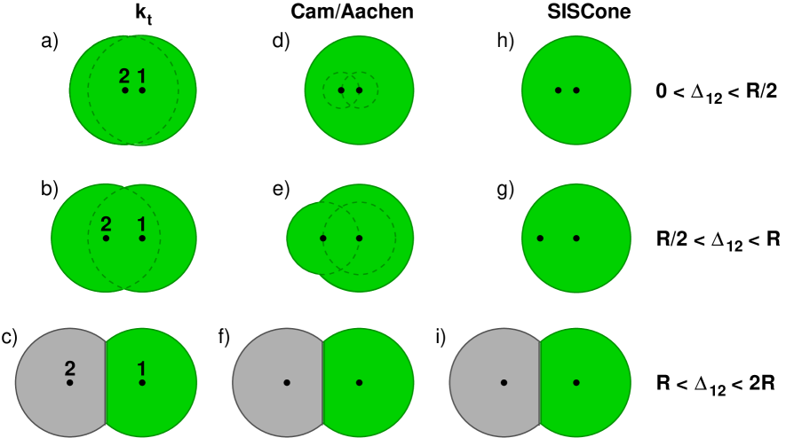
Let us now consider various cases. If , (fig. 1a,b) the particles and will eventually end up in the same jet. The ghost will therefore belong to the jet irrespectively of having been clustered first with or . The area of the jet will then be given by union of two circles of radius , one centred on each of the two perturbative particles,
| (6) |
where
| (7) |
represents the area, divided by , of the union of two circles of radius one whose centres are separated by .
The next case we consider is , fig. 1c. In this case and will never be able to cluster together. Hence, they form different jets, and the ghost will belong to the jet of the closer of or . The two jets will each have area
| (8) |
Finally, for the two jets formed by and each have area .
2.2.2 Cambridge/Aachen
Now we consider the behaviour of the Cambridge/Aachen jet algorithm [15], also a sequential recombination algorithm, defined by the 2-particle distance measure and beam-particle distance . Because in this case the distance measure does not involve the transverse momentum of the particles, the ghost only clusters first if . Otherwise, and cluster first into the jet , and then captures the ghost if .
The region now needs to be separated into two parts, and .
If the ghost clusters first, then it must have been contained in either of the dashed circles depicted in figs. 1d,e. If both these circles are contained in a circle of radius centred on (fig. 1d), and so the jet area is .
If (fig. 1e) the circle of radius centred on protrudes, and adds to the area of the final jet, so that
| (9) |
where
| (10) |
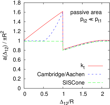
For a Cambridge/Aachen jet has the same area as the jet, cf. fig. 1f. As with the algorithm, the above results are summarised in table 1 and fig. 2. The latter in particular illustrates the significant difference between the and Cambridge/Aachen areas for , caused by the different order of recombinations in the two algorithms.
2.2.3 SISCone
Modern cone jet algorithms identify stable cones and then apply a split/merge procedure to overlapping stable cones. The arguments that follow are identical for midpoint and seedless cone jet algorithms with a Tevatron run II type split–merge procedure [22]. For higher orders, or more realistic events, it is mandatory to use an infrared-safe seedless variant, a main example of which is SISCone [16].
For only a single stable cone is found, centred on . Any ghost within distance of will therefore belong to this jet, so its area will be , cf. fig. 1h,g.
For two stable cones are found, centred on and . The split/merge procedure will then always split them, because the fraction of overlapping energy is zero. Any ghost falling within either of the two cones will be assigned to the closer of and (see fig. 1i). The area of the hard jet will therefore be the same as for the and Cambridge algorithms.
Again these results are summarised in table 1 and fig. 2 and one notices the large differences relative to the other algorithms at and the striking feature that the cone algorithm only ever has negative corrections to the passive area for these energy-ordered two-particle configurations.
| Cambridge/Aachen | SISCone | ||
|---|---|---|---|
2.3 Area scaling violation
Given that jet passive areas are modified by the presence of a soft particle in the neighbourhood of a jet, one expects the average jet area to acquire a logarithmic dependence on the jet transverse momentum when the jets acquire a sub-structure as a consequence of radiative emission of gluons.To determine its coefficient we shall work in the approximation of small jet radii, motivated by the observation that corrections for finite , proportional to powers of , are usually accompanied by a small coefficient [13, 10].
In the small-angle limit, the QCD matrix element for the emission of the perturbative soft gluon, , is
| (11) |
where is or according to whether the hard particle is a quark or a gluon. We make use of the fact that is just the angle between the two particles (to within a longitudinal boost-dependent factor), and will assume that is sufficiently small that the small-angle approximation is legitimate. The scale of the coupling is taken to be the transverse momentum of relative to .
At order the mean jet area with a given jet algorithm (JA) can be written
| (12) |
where we explicitly isolate the higher-order contribution,
| (13) |
with the term accounting for virtual corrections. represents therefore an average over perturbative emission. Note that because of the soft divergence for the emission of , eq. (13) diverges unless one specifies a lower limit on — accordingly we have to introduce an infrared cutoff on the of the emitted gluon. This value results from requiring that the transverse momentum of relative to , i.e. , be larger than . The fact that we need to place a lower limit on means that jet areas are infrared unsafe222An exception is for the SISCone algorithm with a cut, , on the minimum transverse momentum of protojets that enter the split–merge procedure procedure — in that situation is effectively replaced by . — they cannot be calculated order by order in perturbative QCD and for real-life jets they will depend on the details of non-perturbative effects (hadronisation). One can account for this to some extent by leaving as a free parameter and examining the dependence of the perturbative result on .333 One should of course bear in mind that the multi-particle structure of the hadron level is such that a single-gluon result cannot contain all the relevant physics — this implies that one should, in future work, examine multi-soft gluon radiation as well, perhaps along the lines of the calculation of non-global logarithms [30, 31, 5, 6], though it is not currently clear how most meaningfully to carry out the matching with the non-perturbative regime. Despite these various issues, we shall see in section 5 that the single-gluon results work remarkably well in comparisons to Monte Carlo predictions. In that section, we shall also argue that in cases with pileup, the pileup introduces a natural semi-hard (i.e. perturbative) cutoff scale that replaces .
As concerns the finiteness of the integration, all the jet algorithms we consider have the property that
| (14a) | ||||
| (14b) | ||||
so that the integral converges for , and we can place the upper limit at .
After evaluating eq. (13), with the replacement , both in the lower limit of the integral and the argument of the coupling, we obtain
| (15) |
in a fixed coupling approximation, and
| (16) |
with a one-loop running coupling, where . The approximation in the argument of the running coupling in the integrand corresponds to neglecting terms of without any enhancements from logarithms of or .
The results for are
| (17a) | ||||
| (17b) | ||||
| (17c) | ||||
where
| (18) |
with . One notes that the coefficient for the algorithm is non-negligible, given that it is multiplied by the quantity in eq. (15) (or its running coupling analogue), which can be of order . In contrast the coefficients for Cambridge/Aachen and SISCone are much smaller and similar (the latter being however of opposite sign). Thus areas will depend significantly more on the jet than will those for the other algorithms.
The fluctuation of the areas can be calculated in a similar way. Let us define
| (19) |
where we have introduced , despite its being null, so as to facilitate comparison with later results. We then evaluate
| (20) |
where we neglect since it is of . The calculation of proceeds much as for and gives
| (21) |
for running coupling. The results are
| (22a) | ||||
| (22b) | ||||
| (22c) | ||||
We have a hierarchy between algorithms that is similar to that observed for the average area scaling violations, though now the coefficient for Cambridge/Aachen is more intermediate between the other two.
2.4 -particle properties and the Voronoi area
The only algorithm for which one can make any statement about the passive area for a general -particle configuration is the algorithm.
Because of the distance measure, the single ghost will cluster with one of the event particles before any other clustering takes place. One can determine the region in which the ghost will cluster with a given particle, and this is a definition of the area of a particle . Since the ghost-particle clustering will occur before any particle-particle clustering, the jet area will be the sum of the areas of all its constituent particles:
| (23) |
Can anything be said about the area of a particle? The ghost will cluster with the event particle to which it is closest, as long it is within a distance . There exists a geometrical construction known as the Voronoi diagram, which subdivides the plane with a set of vertices into cells around each vertices.444It is this same geometrical construction that was used to obtain a nearest neighbour graph that allowed jet clustering to be carried out in time [23]. Each cell has the property that all points in the cell have as their closest vertex the cell’s vertex. Thus the Voronoi cell is remarkably similar to the region in which a ghost will cluster with a particle. The only difference arises because of the limitation that the ghost should be within a distance of the particle — this causes the area of particle to be the area of its Voronoi cell intersected with a circle of radius , , centred on the particle. This leads us to define a Voronoi area for a particle, ,
| (24) |
Thus given a set of momenta, the passive area of a jet can be directly determined from the Voronoi diagram of the event,555Strictly speaking it should be the Voronoi diagram on a cylinder, however this is just a technical detail. using eq. (23) and the relation
| (25) |
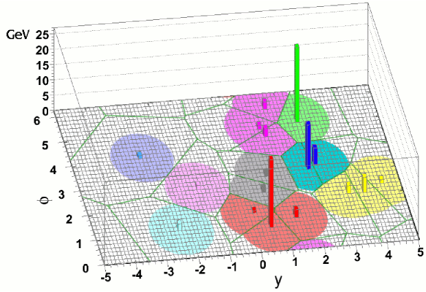
It is quite straightforward to see that this result holds for the 2-particle case, because the Voronoi diagram there consists of a single line, equidistant between the two points. It divides the plane into two half-planes, each of which is the Voronoi cell of one of the particles (this is best seen in fig. 1c). The intersection of the halfplane with the circle of radius centred on the particle has area , and this immediately gives us the results eqs. (6), (8) according to whether the particles cluster into a single jet or not.
The Voronoi construction of the -algorithm passive area is illustrated for a more complex event in fig. 3. One sees both the Voronoi cells and how their intersection with circles of radius gives the area of the particles making up those jets.
Note that it is not possible to write passive areas for jet algorithms other than in the form eq. (23). One can however introduce a new type of area for a generic algorithm, a Voronoi area, in the form
| (26) |
While for algorithms other than (for which, as we have seen, ), this area is not in general related to the clustering of any specific kind of background radiation, it can nevertheless be a useful tool, because its numerical evaluation is efficient [24, 23] and as we shall discuss later (sec. 3.4), for dense events its value coincides with both passive and active area definitions.
3 Active Area
To define an active area, as for the passive area, we start with an event composed of a set of particles which are clustered into a set of jets by some infrared-safe jet algorithm. However, instead of adding a single soft ghost particle, we now add a dense coverage of ghost particles, , randomly distributed in rapidity and azimuth, and each with an infinitesimal transverse momentum.666In most cases the distribution of those transverse momenta will be irrelevant, at least in the limit in which the density of ghosts is sufficiently high. The clustering is then repeated including the set of particles plus ghosts.
During the clustering the ghosts may cluster both with each other and with the hard particles. This more ‘active’ participation in the clustering is the origin of the name that we give to the area to be defined shortly. It contrasts with the definition of section 2, in which the single ghost acted more as a passive spectator, and in particular could not cluster with any other ghosts (there weren’t any).
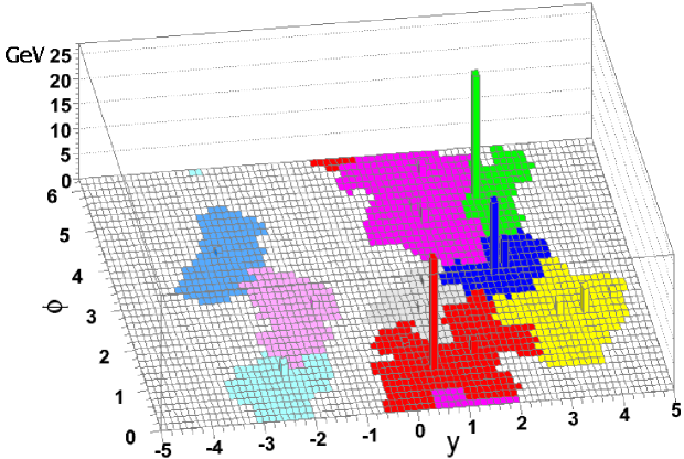
Because of the infrared safety of any proper jet algorithm, even the addition of many ghosts does not change the momenta of the final jets . However these jets do contain extra particles, ghosts, and we use the number of ghosts in a jet as a measure of its area. Specifically, if the number of ghosts per unit area (on the rapidity-azimuth cylinder) is and is the number of ghosts contained in jet , then the (scalar) active area of a jet, given the specific set of ghosts is
| (27) |
An example of jet areas obtained in this way is shown in figure 4. One notes that the boundaries of the jets are rather ragged. Clustering with a different set of ghosts would lead to different boundaries. This is because the ghosts can cluster among themselves to form macroscopic subjets, whose outlines inevitably depend on the specific set of initial ghosts,777This is a form of dynamic magnification of the microscopic local breaking of translational invariance introduced by the ghosts’ randomness. and these then subsequently cluster with true event particles. This can happen for any density of ghosts, and thus the jet boundaries tend, for most algorithms, to be sensitive to the randomness of the initial sets of ghosts.
This randomness propagates through to the number of ghosts clustered within a given jet, even in the limit , resulting in a different area each time. To obtain a unique answer for active area of a given jet one must therefore average over many sets of ghosts, in addition to taking the limit of infinite ghost density,888One may wonder if the averaged area (and its dispersion) depends on the specific nature of the fluctuations in ghost positions and momenta across ensembles of ghosts — for a range of choices of these fluctuations, no significant difference has been observed (except in the case of pure ghost jets with SISCone, whose split–merge step introduces a strong dependence on the microscopic event structure).
| (28) |
Note that as one takes , the ghost transverse momentum density, , is to be kept infinitesimal.
The active area should bear a close resemblance to the average susceptibility of the jet to a high density of soft radiation (e.g. minimum-bias pileup), since the many soft particles will cluster between each other and into jets much in the same way as will the ghosts.
One may also define the standard deviation of the distribution of a jet’s active area across many ghost ensembles,
| (29) |
This provides a measure of the variability of a given jet’s contamination from (say) pileup and is closely connected with the momentum resolution that can be obtained with a given jet algorithm.
A feature that arises when adding many ghosts to an event is that some of the final jets contain nothing but ghost particles. They did not appear in the original list of and we refer to them as pure ghost jets. These ‘ghost’ jets (not shown in fig. 4), fill all of the ‘empty’ area, at least in jet algorithms for which all particles are clustered into jets. They will be similar to the jets formed from purely soft radiation in events with minimum-bias pileup, and so are interesting to study in their own right.
We can also define a 4-vector version of the active area (in analogy with the 4-vector passive area). It is given by
| (30) |
The sum of the is to be understood as carried out in the same recombination scheme as used in the jet clustering.999Though we do not give the details it is simple to extend the 4-vector active area definition to hold also for a general IR safe jet algorithm, in analogy with the extension of the passive area definition in eq. (3).
3.1 Areas for 1-particle configurations and for ghost jets
3.1.1 and Cambridge/Aachen
The active area for the and Cambridge/Aachen algorithms is most readily studied numerically, by directly clustering large numbers of ghost particles, possibly together with one or more hard particles. This is feasible because of the availability of fast computational methods for carrying out the clustering in these algorithms, implemented in the FastJet package [23]. Typically we add ghosts with a density of per unit area,101010They are placed on a randomly scattered grid, in order to limit the impact of the finite density, i.e. one effectively carries out quasi Monte Carlo integration of the ghost ensembles, so that that finite density effects ought to vanish as , rather than as would be obtained with completely random placement. in the rapidity region , and study jets in the region . This leads to about 7500 ghost particles, which can be clustered in about on a processor. Each ghost is given a transverse momentum and the one hard particle that we study has a transverse momentum of . The results are insensitive to the values chosen as long as their ratio is sufficiently large. We investigate in Appendix B how the distribution of the “1-hard-parton” jet area gets modified when the transverse momentum of the parton is progressively reduced below the scale of a generic set of soft particles.
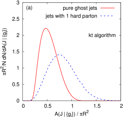
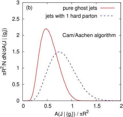
Figure 5 shows the distribution of values of for pure ghost jets and jets with one hard particle. The distribution is obtained over a large ensemble of sets of ghosts.111111In this particular case we have used about separate random ghost sets, in order to obtain a smooth curve for the whole distribution. When calculating areas in physical events (or even at parton-shower level) the multiple real particles in the jet “fix” most of the area, and between 1 and 5 sets of ghosts particles are usually sufficient to obtain reliable area results (this is the case also for SISCone). Let us concentrate initially on the case with a hard particle. Firstly the average active area, eq. (28) differs noticeably from the passive result of :
| (31a) | ||||
| (31b) | ||||
Secondly, the distributions of the area in fig. 5 are rather broad. The randomness in the initial distribution of ghosts propagates all the way into the shape of the final jet and hence its area. This occurs because the and Cambridge/Aachen algorithms flexibly adapt themselves to local structure (a good property when trying to reconstruct perturbative showering), and once a random perturbation has formed in the density of ghosts this seeds further growth of the soft part of the jet. The standard deviations of the resulting distributions are
| (32a) | ||||
| (32b) | ||||
Figure 5 also shows the distribution of areas for pure ghost jets. One sees that pure ghost jets typically have a smaller area than hard-particle jets:121212Obtaining these values actually requires going beyond the ghost density and the rapidity range previously mentioned. In fact, when going to higher accuracy one notices the presence of small edge and finite-density effects, and to some given power. Choosing the ghost area sufficiently small to ensure that finite-density effects are limited to the fourth decimal (in practice this means ) and extrapolating to infinite one finds (33a) (33b) with a conservative estimate of the residual uncertainty. This points to a small but statistically significant difference between the two algorithms.
| (34a) | ||||
| (34b) | ||||
and the standard deviations are
| (35a) | ||||
| (35b) | ||||
The fact that pure ghost jets are smaller than hard jets has an implication for certain physics studies: one expects jets made of soft ‘junk’ (minimum bias, pileup, thermal noise in heavy ions) to have area properties similar to ghost jets; since they are smaller on average than true hard jets, the hard jets will emerge from the junk somewhat more clearly than if both had the same area.
3.1.2 SISCone
The SISCone algorithm is unique among the algorithms studied here in that its active area is amenable to analytical treatment, at least in some cases.
We recall that a modern cone algorithm starts by finding all stable cones. One stable cone is centred on the single hard particle. Additionally, there will be a large number of other stable cones, of order of the number of ghost particles added to the event [16]. In the limit of an infinite number of ghosts, all cones that can be drawn in the rapidity-azimuth plane and that do not overlap with the hard particle will be stable. Many of these stable cones will still overlap with the cone centred on the hard particle, as long as they do not contain the hard particle itself (see figure 6, left).
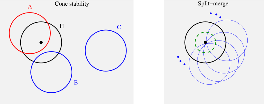
Next, the SISCone algorithm involves a split–merge procedure. One defines for a jet as the scalar sum of the transverse momenta of its constituents. During the split–merge step, SISCone finds the stable cone with the highest , and then the next hardest stable cone that overlaps with it. To decide whether these two cones (protojets) are to be merged or split, it determines the fraction of the softer cone’s that is shared with the harder cone. If this fraction is smaller than some value (the overlap parameter of the cone algorithm), the two protojets are split: particles that are shared between them are assigned to the protojet to whose centre131313This centre is given by the sum of momenta in the protojet before the split–merge operation. they are closer. Otherwise they are merged into a single protojet. This procedure is repeated until the hard protojet no longer has any overlap with other protojets. At this point it is called a jet, and the split–merge procedure continues on the remaining protojets (without affecting the area of the hard jet).
The maximum possible overlap fraction,141414The fraction of momentum coincides with the fraction of area because the ghosts have uniform transverse momentum density. , between the hard protojet and a ghost protojet occurs in the situation depicted in figure 6 (right), i.e. when the ghost protojet’s centre is just outside the edge of the original hard stable cone (H). It is given by . This means that for a split–merge parameter (commonly used values are and ) every overlap between the hard protojet and a pure-ghost stable cone will lead to a splitting. Since these pure-ghost stable cones are centred at distances from the hard particle, these splittings will reduce the hard jet to a circle of radius (the dashed green line in the right hand part of figure 6). The active area of the hard jet is thus
| (36) |
This result has been verified numerically using the same technique employed above for and Cambridge/Aachen.
Note that this area differs considerably from the passive area, . This shows that the cone area is very sensitive to the structure of the event, and it certainly does not always coincide with the naive geometrical expectation , contrary to assumptions sometimes made in the literature (see for example [25]).
We further note that in contrast to and Cambridge/Aachen algorithms, the SISCone algorithm always has the same active area for a single hard particle, independently of fluctuations of an infinitely dense set of ghosts, i.e.
| (37) |
SISCone ghost-jet areas.
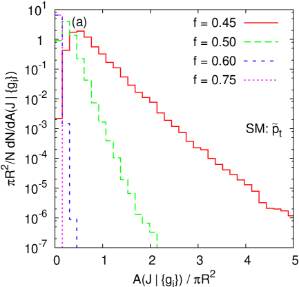
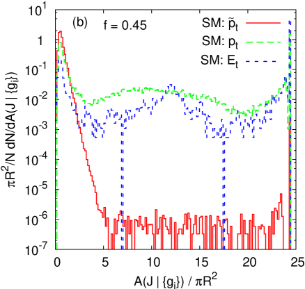
While the area of a hard particle jet could be treated analytically, this is not the case for the pure-ghost jet area. Furthermore, numerical investigations reveal that the pure-ghost area distribution has a much more complicated behaviour than for or Cambridge/Aachen. One aspect is that the distribution of pure-ghost jet areas is sensitive to the fine details of how the ghosts are distributed (density and transverse momentum fluctuations). Another is that it depends significantly on the details of the split–merge procedure. Figure 7a shows the distribution of areas of ghost jets for SISCone, for different values of the split–merge overlap threshold . One sees, for example, that for smaller values of there are occasional rather large ghost jets, whereas for nearly all ghost jets have very small areas.
One of the characteristics of SISCone that differs from previous cone algorithms is the specific ordering and comparison variable used to determine splitting and merging. As explained above, the choice made in SISCone was , the scalar sum of transverse momenta of all particles in a jet. Previous cone algorithms used either the vector sum of constituent transverse momenta, (an infrared unsafe choice), or the transverse energy (in a 4-vector recombination scheme). With both of these choices of variable, split–merge thresholds can lead to the formation of ‘monster’ ghost jets, which can even wrap around the whole cylindrical phase space. For this is a quite frequent occurrence, as illustrated in figure 7b, where one sees a substantial number of jets occupying the whole of the phase space (i.e. an area ). Monster jets can be formed also with the choice, though it is a somewhat rarer occurrence — happening in ‘only’ of events.151515This figure is not immediately deducible from fig. 7b, which shows results normalised to the total number of ghost jets, rather than to the number of events.
We have observed the formation of such monster jets also from normal pileup momenta simulated with Pythia [18], indicating that this disturbing characteristic is not merely an artefact related to our particular choice of ghosts. This indicates that a proper choice of the split–merge variable and threshold is critical in high-luminosity environments. The results from Figure 7a, suggest that if one wants to avoid monster jets, one has to choose a large enough value for . Our recommendation is to adopt as a default value for the split–merge threshold (together with the use of the variable, already the default in SISCone, for reasons related to infrared safety and longitudinal boost invariance).
3.2 Areas for 2-particle configurations
In this section we study the same problem described in section 2.2, i.e. the area of jets containing two particles, a hard one and a softer (but still “perturbative”) one, i.e. eq. (4), but now for active areas. As before, the results will then serve as an input in understanding the dependence of the active area on the jet’s transverse momentum when accounting for perturbative radiation.
3.2.1 and Cambridge/Aachen
As was the case for the active area of a jet containing a single hard particle, we again have to resort to numerical analyses to study that of jets with two energy-ordered particles. We define to be the active area for the energy-ordered two particle configuration already discussed in section 2.2.
Additionally since we have a distribution of areas for the single-particle active area case, it becomes of interest to study also the standard deviation of the distribution of areas obtained for the two-particle configuration.
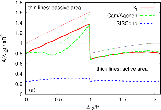
The results are shown in figure 8: the active areas can be seen to be consistently smaller than the passive ones, as was the case for the 1-particle area, but retain the same dependence on the angular separation between the two particles. Among the various features, one can also observe that the active area does not quite reach the single-particle value () at , but only somewhat beyond . This contrasts with the behaviour of the passive area. The figure also shows results for the cone area, discussed in the following subsection.

3.2.2 SISCone
In the case of the SISCone algorithm it is possible to find an analytical result for the two-particle active area, in an extension of what was done for one-particle case.161616This is only possible for configurations with strong energy ordering between all particles — as soon as 2 or more particles have commensurate transverse momenta then the cone’s split–merge procedure will include ‘merge’ steps, whose effects on the active area are currently beyond analytical understanding.
The stable-cone search will find one or two “hard” stable cones: the first centred on the hard particle and the second centred on the soft one, present only for . The pure-ghost stable cones will be centred at all positions distant by more than from both and , i.e. outside the two circles centred on and .
We shall consider the active area of the jet centred on the hard particle . When , the jet centred on the soft particle has the same area.
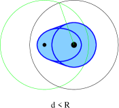
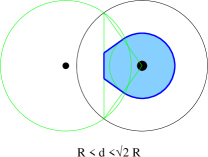
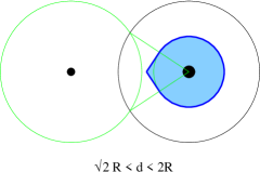
As in section 3.1.2, the split–merge procedure first deals with the pure-ghost protojets overlapping with the hard stable cone. For , this again only leads to splittings. Depending of the value of , different situations are found as shown on figure 9. If the - coordinates of the particles are and , the geometrical objects that are present are: the circle centred on with radius ; the tangents to this circle at - coordinates ; and, for , the ellipse of eccentricity whose foci are and (given by the equation, , where is a point on the ellipse). For the area of the jet is given by the union of the ellipse, the circle and the regions between the ellipse, the circle and each of the tangents (fig. 9a). For it is given by the circle plus the region between the circle, the two tangents and the line equidistant from and (fig. 9b). For it is given by the circle plus the region between the circle and two tangents, up to the intersection of the two tangents (fig. 9c). Finally, for , the area is .
An analytic computation of the active area gives
with , while for , one recovers the result . The SISCone active area is plotted in figure 10 and it is compared to the results for and Cambridge/Aachen in figure 8. One notes that the SISCone result is both qualitatively and quantitatively much further from the passive result than was the case for and Cambridge/Aachen.
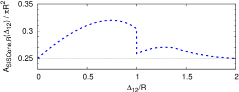
The main reason why the 2-point active area is larger than the 1-point active area (whereas we saw the opposite behaviour for the passive areas) is that the presence of the 2-particle configuration causes a number of the pure-ghost cones that were present in the 1-particle case to now contain the second particle and therefore be unstable. Since these pure ghost cones are responsible for reducing the jet area relative to the passive result (during the split–merge step), their absence causes the active area to be ‘less-reduced’ than in the 1-particle case.
3.3 Area scaling violation
We can write the order contribution to the average active area in a manner similar to the passive area case, eq. (13):
| (39) |
where we have used the relation and where
| (40) |
Note that compared to eq. (13) we have removed the explicit upper limit at on the integral since, for active areas of sequential recombination algorithms, may be non zero even for . Note also the notation for averages: we use to refer to an average over perturbative emissions, while , implicitly contained in (see eq. (28)), refers to an average over ghost ensembles. We now proceed as in section 2.3, and write
| (41) |
where for brevity we have given just the running-coupling result. One observes that the result continues to depend on , an indication that the active area is an infrared-unsafe quantity, just like the passive area.171717We believe that any sensible (i.e. related to the jet’s sensitivity to UE/pileup type contamination) definition of area would actually be infrared unsafe. The coefficients for the anomalous dimension of the active area for the various algorithms are
| (42a) | ||||
| (42b) | ||||
| (42c) | ||||
where the SISCone result has been obtained by integrating the analytical result, eq. (3.2.2), while the results for and Cambridge/Aachen have been obtained both by integrating the 2-point active-area results shown in fig. 8 and by a direct Monte Carlo evaluation of eq. (41). Note that while the coefficients for and Cambridge/Aachen are only slightly different from their passive counterparts, the one for SISCone has the opposite sign relative to the passive one.
The treatment of higher-order fluctuations of active areas is more complex than that for the passive ones, where the one-particle area was a constant. We can separate the fluctuations of active areas into two components, one (described above) that is the just the one-particle result and the other, , accounting for their modification in the presence of perturbative radiation:
| (43) |
where is given by eqs. (32a,b) for the and the Cambridge/Aachen algorithms respectively, and it is equal to zero for the SISCone algorithm. The perturbative modification is itself now driven by two mechanisms: the fact that the second particle causes the average area to change, and that it also causes modifications of the fluctuations associated with the sampling over many ghost sets. We therefore write
| (44) | ||||
| (45) | ||||
| (46) |
where as usual we neglect contributions that are not enhanced by any logarithm or that are higher-order in . The details of how to obtain these results are given in Appendix C.
The coefficient can be determined only numerically for the and Cambridge/Aachen algorithms, while for the SISCone algorithm the result can be deduced from eq. (3.2.2) together with the knowledge that :
| (47a) | ||||
| (47b) | ||||
| (47c) | ||||
Again, both the values and their ordering are similar to what we have obtained for the passive areas (see eq. (22)).
3.4 -particle properties and large- behaviour
3.4.1 algorithm
As for the passive area, the algorithm’s active area has the property that it can be expressed as a sum of individual particle areas:
| (48) |
This is the case because the presence of the momentum scale in the distance measure means that all ghosts cluster among themselves and with the hard particles, before any of the hard particles start clustering between themselves. However in contrast to the passive-area situation, there is no known simple geometrical construction for the individual particle area.
3.4.2 Equivalence of all areas for large
The existence of different area definitions is linked to the ambiguity in assigning ‘empty space’ to any particular jet. In the presence of a sufficiently large number of particles , one expects this ambiguity to vanish because real particles fill up more and more of the empty space and thus help to sharpen the boundaries between jets. Thus in the limit of many particles, all sensible area definitions should give identical results for a given jet.
To quantify this statement, we examine (a bound on) the scaling law for the relation between the density of particles and the magnitude of the potential differences between different area definitions. We consider the limit of ‘dense’ coverage, defined as follows: take square tiles of some size and use them to cover the rapidity–azimuth cylinder (up to some maximal rapidity). Define as the smallest value of tile edge-length such that all tiles contain at least one particle. In an event consisting of uniformly distributed particles, is of the same order of magnitude as the typical interparticle distance. The event is considered to be dense if .
Now let us define a boundary tile of a jet to be a tile that contains at least one particle of that jet and also contains a particle from another jet or has an adjacent tile containing one or more particle(s) belonging to a different jet. We expect that the difference between different jet-area definitions cannot be significantly larger than the total area of the boundary tiles for a jet.
The number of boundary tiles for jets produced by a given jet algorithm (of radius ) may scale in a non-trivial manner with the inter-particle spacing , since the boundary may well have a fractal structure. We therefore parametrise the average number of boundary tiles for a jet, as
| (49) |
where the fractal dimension would correspond to a smooth boundary. The total area of these boundary tiles gives an upper limit on the ambiguity of the jet area
| (50) |
and similarly for the difference between active or passive and Voronoi areas. As long as the differences between various area definitions are guaranteed to vanish in the infinitely dense limit, . We note that corresponds to a situation in which the boundary itself behaves like an area, i.e. occupies the same order of magnitude of space as the jet itself. This would be visible in plots representing jet active areas (such as fig. 4), in the form of finely intertwined jets. We have seen no evidence for this and therefore believe that for all three jet algorithms considered here.
In practice we expect the difference between any two area definitions to vanish much more rapidly than eq. (50) as , since the upper bound will only be saturated if, for every tile, the difference between two area definitions has the same sign. This seems highly unlikely. If instead differences in the area for each tile are uncorrelated (but each of order ) then one would expect to see
| (51) |
We have measured the fractal dimension for the and Cambridge/Aachen algorithms and find .181818This has been measured on pure ghost jets, because their higher multiplicity facilitates the extraction of a reliable result, however we strongly suspect that it holds also for single-particle jets. Note that any measurement of the fractal dimension of jet algorithms in real data would be severely complicated by additional structure added to jets by QCD branching, itself also approximately fractal in nature.
The fact that active and passive (or Voronoi) areas all give the same result in dense events has practical applications in real-life situations where an event is populated by a very large number of particles (heavy ion collisions being an example). In this case it will be possible to choose the area type which is fastest to compute (for instance the Voronoi area) and use the results in place of the active or passive one.
4 Back reaction
So far we have considered how a set of infinitely soft ghosts clusters with a hard jet, examining also cases where the jet has some finitely-soft substructure. This infinitely-soft approximation for the ghosts is not only adequate, but also necessary from the point of view of properly defining jet areas. However if we are to understand the impact of minimum-bias (MB) and underlying-event radiation on jet finding — the original motivation for studying areas — then we should take into account the fact that these contributions provide a dense background of particles at some small but finite soft scale .
This has two main consequences. The first (more trivial) one is that the minimum-bias or underlying event can provide an alternative, dynamic infrared cutoff in the integration in equations such as eq. (13): assuming that the density of MB transverse momentum per unit area is given by then one can expect that when , the presence of will no longer affect the clustering of the ghosts (i.e. the MB particles). In this case the integral will then acquire an effective infrared cutoff and in expressions such as eqs. (15,16), will be replaced by . Note that neither with infinitely nor finitely-soft ghosts do we claim control over the coefficient in front of this cutoff, though we do have confidence in the prediction of its dependence for small .191919The coefficient can actually be determined quite straightforwardly, however since its impact is of the same order as other effects that we neglect (i.e. free of any logarithmic enhancements) we leave its determination to future work.
The second consequence of the finite softness of the MB contribution is that the addition of the MB particles can modify the set of non-MB particles that make it into a jet. We call this ‘back-reaction’ and it is the main subject of this section.
That back reaction should happen is quite intuitive as concerns non-MB particles whose softness is commensurate with the MB scale. However the extent to which it occurs depends significantly on the jet algorithm. Furthermore for some algorithms it can also occur (rarely) even for non-MB particles that are much harder than the MB scale.
As with the studies of areas, there are two limits that can usefully be examined for back-reaction: the illustrative and mathematically simpler (but less physical) case in which the MB is pointlike and the more realistic case with diffuse MB radiation.
4.1 Back reaction from pointlike minimum-bias
Let us first calculate back reaction in the case of pointlike minimum bias. We will consider minimum-bias particles with transverse momentum distributed uniformly on the – cylinder with density . We use a subscript rather than to differentiate them from ghost particles, the key distinction being that is small but finite, where is infinitesimal.
Let us consider the situation in which a particle , with large transverse momentum, , has emitted a soft particle on a scale commensurate with the minimum-bias particles, . We shall calculate the probability that was part of the jet in the absence of the minimum-bias particle, but is lost from it when the minimum-bias particle is added. This can be written
| (52) |
where is () if, in the absence of , is inside (outside) the jet that contains . Similarly, is () if, in the presence of , is inside (outside) the jet that contains . One can also define the probability for to not be part of the jet in the absence of the minimum-bias particle, but to be gained by the jet when the minimum-bias particle is added,
| (53) |
It is convenient to factor out the particle production probability as follows, in the small limit,
| (54) |
where can be thought of as the effective ‘back-reaction area’ over which the minimum-bias particle causes a loss of jet contents, given a angular distribution for the jet contents:202020Strictly speaking it is the integral over area of the probability of causing a loss of jet contents.
| (55) |
One can similarly define an effective back-reaction area for gain,
| (56) | ||||
| (57) |
For sequential-recombination algorithms the functions in eqs. (55,57) translate to a series of -functions, e.g.
| (58) |
for the algorithm and
| (59) |
for Cambridge/Aachen, where is the distance between and the recombined . Evaluating integrals with the above -functions is rather tedious, but one can usefully consider the limit . This of physical interest because it relates to the probability that the minimum-bias particle induces changes in jet momentum that are much larger than , and a number of simplifications occur in this limit. Since
| (60) |
must be close to the edge of the jet in order for it to be pulled out by , . Without loss of generality, we can set , so that , and
| (61) |
We can then carry out the integrations over and straightforwardly, leading to following the result for loss at high ,
| (62) |
In a similar manner one obtains for the gain,
| (63) |
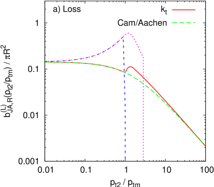
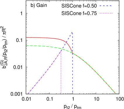
The results for general , determined numerically, are shown in figure 11. The SISCone results are included and have the property that ,
| (64a) | ||||
| (64b) | ||||
i.e. at high , point-like minimum bias never induces back-reaction in the cone algorithm,212121For large but finite , back-reaction can actually occur beyond the above limits, but only with probability . in contrast to the situation with the sequential recombination algorithms, for which back-reaction occurs with a suppressed, but non-zero probability . On the other hand, for back-reaction is more likely with the cone algorithm — the effective area over which the MB particle can cause a change in jet contents is , to be compared to for the and Cambridge/Aachen algorithms.
One may use the results eqs. (62)–(64) to determine the average change in jet-momentum due to back reaction. Because of the logarithmic spectrum of emissions , one finds that it receives contributions from the whole logarithmic region ,
| (65) |
(evaluated for fixed coupling), where corresponds to the average transverse momentum of minimum-bias radiation per unit area and
| (66) |
The structure of the correction in eq. (65) is very similar to that for the actual contamination from minimum bias, , with as determined in section 2.3: notably, for fixed coupling, the average back-reaction scales with the logarithm of the jet . The coefficients ,
| (67a) | ||||
| (67b) | ||||
can be directly compared to the results for the there. The values are relatively small, similar in particular to what one observes for the Cambridge/Aachen algorithm, though of opposite sign.
Though the average change in jet momentum, both from scaling violations of the area and from back-reaction, have a similar analytical structure, it is worth bearing in mind that these similar analytical structures come about quite differently in the two cases. Regarding area scaling violations, a significant fraction of jets, , are subject to a change in area (cf. section 2.3), and a consequent modification of the minimum-bias contamination by a modest amount . In contrast the average back reaction effect , is due to large modifications of the jet momentum with occurring rarely, with a differential probability that depends on as . One consequence of this is that the mean square change in transverse momentum due to back-reaction is dominated by very rare modifications of jets in which , giving
| (68) |
Note that the coefficient of this dispersion is non-zero even for the SISCone algorithm, due to the residual probability that it has, for finite , for any change in structure with .
4.2 Back reaction from diffuse MB
Let us now examine back reaction in the case where the minimum-bias radiation has a uniform diffuse structure, consisting of a high density of minimum-bias particles, . The relation between back reaction in the point-like and diffuse cases is rather similar to the relation between passive and active areas: key analytical features remain unaffected by the change in the structure of the minimum bias, but certain specific coefficients change.
We define the probability for loss in the presence of diffuse MB as
| (69) |
where the average is performed over the ensemble of MB configurations, and now is 1 (0) if is outside (inside) the jet containing in the presence of the specific minimum-bias instance. A similar equation holds for the gain probability.
Then, as with eq. (54) we factorise this,
| (70) |
into one piece related to the probability for perturbative emission and a second piece that is the diffuse analogue of the effective back-reaction area in the point-like case. Note however that it is not so obvious exactly what geometrical area actually corresponds to.222222A related issue is that the precise choice of normalisation of is somewhat arbitrary — our specific choice is intended to provide a meaningful connection with in the large limit. Similarly, we introduce and corresponding to the gain in the presence of a diffuse MB.
The only case for which we have analytical results for is the SISCone algorithm, for which (with )
| (71) |
This is a consequence of the facts (a) that the addition of a uniform background of MB particles has no effect on the stability (or instability) of a specific cone, (b) that for the split–merge step is immaterial to the jet finding if is within the cone around , and (c) that for outside the cone around , the maximal possible overlap is of ’s stable cone with that of is and if then the two cones will always be split, ensuring that remains in a jet distinct from . We believe that real-life corrections to the zero in eq. (71) are proportional to the standard deviation of MB transverse-momentum density from point to point in the event.
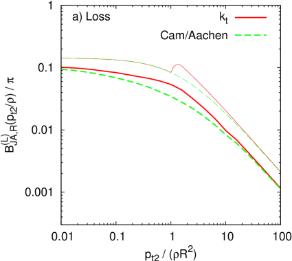
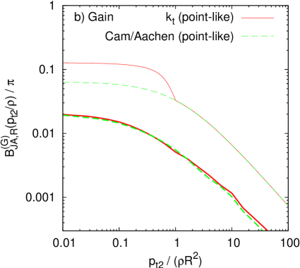
Numerical results for the for the and Cambridge/Aachen algorithms are given in in figure 12 and compared to the results in the point-like case. One sees that the general functional form is rather similar though the normalisations are somewhat smaller (by a factor of for loss, a factor for gain). The asymptotic large- behaviours are observed to be
| (72a) | ||||
| (72b) | ||||
As in the point-like case we can calculate the mean change in jet transverse momentum due to back reaction and we obtain
| (73) |
with
| (74) |
Even though had as its argument and has , the final expressions for the average back-reaction in the point-like and diffuse cases, eqs. (65), (73), have almost identical forms — in particular the overall scale appearing in each is and the only difference appears in the denominator for the argument of the logarithm. The coefficients are slightly smaller,
| (75a) | ||||
| (75b) | ||||
and will again translate to modest effects compared to the overall minimum-bias contamination in the jets. Note also however that in general the scaling with of and is subtly different. The former truly behaves like an area, in that is -independent; the latter instead has the property that it is that is -independent.
5 Areas in (simulated) real life
In this section we shall examine the properties of jet areas in the context of realistic events, as simulated with Herwig [17] and Pythia [18]. There are two purposes to doing so. Firstly we wish to illustrate the extent to which the simple single-gluon emission arguments of the previous section hold once one includes full parton-showering and hadronisation. Secondly, jet areas have the potential to play an important role in the estimation and subtraction of underlying event and pileup contamination, as discussed in [19]. The study of jet areas in realistic events can help to highlight some of the issues that arise in such a procedure.
5.1 Jet area distributions and anomalous dimension
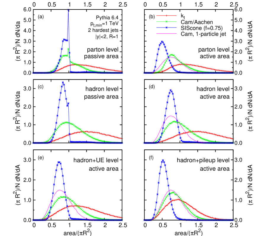
Let us start with an investigation of the distribution of the areas of hard jets with in simulated LHC dijet events, fig. 13. The area distributions are shown for various ‘levels’ in the Monte Carlo: just after parton showering, after hadronisation, both with and without an UE, and finally with a substantial pileup contribution (high-luminosity LHC, interactions per bunch crossing). We examine both passive and active areas.
The passive areas distributions at parton-shower level, fig. 13a, are those that are most amenable to understanding in terms of our analytical results. Firstly one notes that the SISCone and Cambridge/Aachen algorithms have a clear peak at . These two algorithms both have the property (cf. section 2.2) that the area is not affected by moderately collinear ( for SISCone, for Cambridge/Aachen) soft particle emission. Thus it is possible, even in the presence of parton showering (which is mostly collinear), for the passive area to remain . For the cone algorithm, the other main structure is a “shoulder” region , which coincides nicely with the range of values that can be induced by 2-particle configurations (cf. fig. 2). A similar shoulder exists for the Cambridge algorithm, which however additionally has jets with — again the range of values spanned, up to , is rather similar to what would be expected from the two-particle calculations. Further broadening of these distributions at the edges is attributable to parton-level states with more than two particles. In contrast the parton-level passive area distribution for the algorithm seems less directly related to the -particle calculations of section 2.2. This can be understood by observing that the passive area is modified even by rather collinear emissions, and the multiple collinear emissions present in parton showers add together to cause substantial broadening of the area distribution.
At parton shower level, there are relatively few particles in the event and there is no obvious boundary to the jet — the ghosts that we add provide a way of assigning that empty area. It is therefore not surprising to see significant differences between the two ways of adding ghosts, i.e. the passive and active area distributions. This is most marked for SISCone, as is to be expected from the results of section 3.1.2, which showed that for a 1-particle jet the active area is . There is a trace of this result in fig. 13b, where one sees that the SISCone distribution now extends down to . There is however no peak structure, presumably because even a highly collinear emission gives a slight modification of the area, cf. fig. 10 (the same argument given for the absence of a peak for the passive area). For the Cambridge/Aachen and algorithms, there is less difference between active and passive area distributions, again as expected.
As one moves to events with more particles, for example hadron level, fig. 13c and d, the particles themselves start to give a clearer outline to the jets. Thus the passive and active distributions are far more similar. This is less so for SISCone than the others, as is to be expected, for which one still sees a trace of the peak at .
For events with many particles, for example with the UE (fig. 13e) and then pileup (fig. 13f) added, the difference between passive and active area distributions is so small that we show only the active area result. These last two plots are the most relevant to phenomenology. A feature of both is that the dispersion is smallest for SISCone (but significantly different from zero) and largest for , precisely as one would expect from eqs. (43) and (47). Another feature is how for Cambridge/Aachen the dispersion is essentially that associated with , the distribution being very similar to the 1-parton active area result, shown as the solid line. This similarity is strongest when there is pileup: the logarithmic enhancement that enters in eq. (44) is reduced because the pileup introduces a large value for . In this case even the algorithm starts to have a distribution of areas that resembles the -parton active area result, and for SISCone one once again sees signs of the lower limit at , the one-particle active area result.
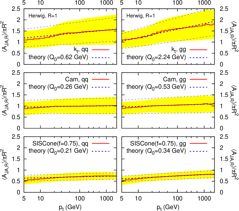
While the plots of fig. 13 provide an illustration of many of the features that we have discussed in the earlier sections of this paper, the fact that we have not systematically calculated area distributions means that the discussion necessarily remains qualitative. For quantitative checks, one should instead examine the mean active area and its dispersion and compare them to the results of section 3. This is done in fig. 14, separately for and for scattering, as a function of the jet transverse momentum. The horizontal scale has been chosen uniform in so that our predictions correspond to straight lines.
The predictions of section 3 set the slope of those lines for each algorithm, and the agreement is reasonable in all cases. The infrared cutoff scale is not predicted, and may differ both between quark and gluon jets and between algorithms. The values for have therefore been fitted, using the results for the mean, and are consistent with a general non-perturbative origin (modulo issues in SISCone discussed below). The standard deviation (indicated by the band for the Monte Carlo simulation and the thin dashed lines for the theory result) is then entirely predicted, and also agrees remarkably well. Thus, overall, our simple analytical calculations provide a surprisingly successful picture of the mean and dispersions for various algorithms, over a range of jet transverse momenta. This is all the more striking considering that the calculation is based on just the first term in a series , and is in part based on a small angle approximation.
Some remarks are due regarding the values. Two clear patterns emerge: it is largest for , smallest for SISCone, and systematically larger for gluon jets than for quark jets. In the case of SISCone with quark jets, the value is uncomfortably close to the value of used in the one-loop coupling. It may be that this low value is an artefact whose origin lies in the finite density both of actual event particles and of ghosts (the latter due to speed limitations in SISCone): when one has a limited density of particles and/or ghosts, the measured area may be intermediate between the passive and “ideal” active areas; because SISCone has such a large difference between passive and active areas (a factor of 4 for the 1-particle results), the finite density effects can be significant, and so may be taking an extreme value in order to compensate for this.
A final comment concerns the choice of event generator. Here we have shown results from Herwig (v. 6.5). Pythia with the original shower (the default choice in v. 6.4) is known to have difficulties reproducing anomalous dimensions associated with soft large angle radiation [26, 27], whereas the new shower [28] mostly resolves these issues [27]. Similar concerns are potentially relevant here too. We actually find that both Pythia showers give results similar to Herwig’s (and ours) in all cases except the algorithm, for which both Pythia showers give a slope a factor of two smaller than expected. This suggests that an experimental measure of the dependence of jet areas might provide some non-trivial constraints on parton-showering dynamics.
5.2 Jet areas and pileup subtraction
One of the main uses of measured jet areas is in the subtraction of pileup [19]. As we have seen there are two contributions to the modification of a jet’s in the presence of pileup: the pileup particles can end up in the jet, and assuming a roughly uniform distribution of pileup (as in the case in the limit of many simultaneous minimum-bias collisions), the resulting change in jet will be proportional to the jet’s area, by definition. Of course the pileup is not exactly uniform in a given event and this must also be accounted for. The only other modification of the jet’s comes from the back reaction. This gives us the following equation for the modification of a jet’s transverse momentum in the presence of pileup, originally stated in [19],
| (76) |
where, as before, is the mean amount of transverse momentum per unit area that has been added to the event by pileup; measures the fluctuations of the pileup from point-to-point within the event (defined as the standard deviation of the distribution of pileup across many squares of area ); and is the net change in transverse momentum due to back reaction. An important point here is that is the area of the jet after the pileup has been added — the fact that the area is not an IR safe quantity means that it is not the same before and after pileup, and it is in the latter case that it correctly measures how much pileup will have entered the jet.
The fluctuations in the jet due to the direct pileup contribution can be written
| (77) |
where the area-related averages are those for events including the pileup (i.e. in calculations of anomalous dimensions), and we separately account both for point to point fluctuations of the pileup within an event (second term), as well as fluctuations in the overall level of pileup from event to event (third term).
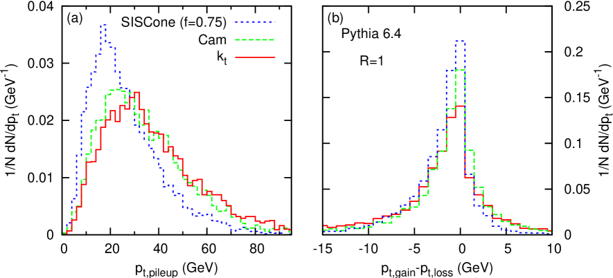
The direct pileup contribution to a sample of jets is shown in fig. 15a corresponding to about interactions per bunch crossing (high-luminosity LHC), as simulated with Pythia tune A. One observes that SISCone has smaller average pileup contamination and smaller fluctuations in this contamination, which is consistent with our analytical calculations. More surprisingly, at least at first sight, has only slightly larger and broader pileup contamination than Cambridge/Aachen, despite its larger area. However its area is generally larger only because of the anomalous dimension: since the logarithm that appears in the anomalous dimension with pileup, , is not very large, the difference between and Cambridge/Aachen is essentially absent. This is visible also in fig. 13f (the somewhat larger difference there is a consequence of the larger jet ).
The reader may have observed that we omitted the back-reaction term in eq. (77). The tail of the distribution for has the property , so the standard deviation is dominated by large , giving a contribution to to eq. (77) of order . For large this is parametrically bigger than the direct pileup contributions, however it is dominated by extremely rare events (those in which a hard particle in the jet is just near the edge of the jet), a fraction of of all events. Consequently it provides a poor estimate of the typical back-reaction.
The actual distribution for the back reaction is shown in fig. 15b, and one sees that the change in momentum is nearly always limited to a few GeV, centred close to zero. It is slightly skewed towards loss, which is consistent with the larger loss than gain probabilities found in section 4.232323Actually, for the and Cambridge/Aachen algorithms, one can verify that the high- tails of the distributions are consistent with the expectation from section 4.2. Actual pileup is not perfectly uniform and for this reason the back-reaction with SISCone is not exactly zero as would have been expected from section 4.2 for diffuse radiation. Nevertheless the gain in particular is smaller than for other algorithms, which happens to coincide with what we would expect from fig. 11 for loss and gain with pointlike pileup.
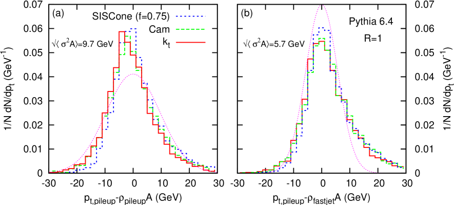
Let us finally come to the question of subtraction of pileup. The equation proposed in [19] was
| (78) |
There we estimated from the event itself and effectively subtracted both UE and pileup. Here let us estimate purely from the pileup particles (with Monte Carlo simulations this is possible) and compare the difference between the added by the pileup and the removed by the our subtraction procedure. The distribution of this difference is shown in fig. 16. The two plots correspond to two different ways of measuring (either directly from the scalar sum of ’s of pileup particles, left, or with the median-based method of [19], which is applicable also in data). In both cases the distributions are clearly centred on zero, indicating a successful subtraction of the pileup.
Of the fluctuation terms in eq. (77), only the middle piece should remain after subtraction. This is consistent with the distributions being much narrower than those in fig. 15a. This is an important point as it means that, in addition to subtracting the average contamination due to pileup, we also reduce its effect on the fluctuations. For example, if one wants to look at the top mass spectrum, the corresponding peak will appear narrower (and with a better signal-to-background ratio) after subtraction than before. As a quantitative test, in fig. 16, we show also a Gaussian of width . Here has been estimated in each event again either directly or with the methods of [19]. Whereas the values obtained with the two methods are similar, those for differ noticeably. This may in part be due to an occasional, hard pointlike contribution in the minimum-bias events, causing the fluctuations measured by to be non-Gaussian. This would explain why the statistically more standard evaluation of shown in Fig. 16a leads to slightly too broad a distribution. In contrast the evaluation of [19], in Fig. 16b, is designed specifically to be insensitive to the pointlike component, on the grounds that one wants a measure not influenced by the main hard scatter. It provides a reasonable estimate of the lower half of the distribution, but undershoots the (asymmetric) upper tail, which one can probably ascribe to the rare pointlike component of the minimum bias collisions.
6 Conclusions
The concept of a jet area is one that initially seems rather intuitive. Yet, as we have seen in this article, there is a wealth of physics associated with it, both in terms of how one defines it and as concerns the interplay between a jet’s internal structure and its area. This is reflected in the range of quantities that can be studied to characterize the behaviour of jet areas, summarised in table 2.
Our guiding principle in defining jet areas has been that they should provide a measure of a jet’s susceptibility to additional underlying event and pileup radiation, in the limit in which these are infinitely soft. Two opposite hypotheses for the structure of such radiation, pointlike or diffuse, lead to two definitions of the area, respectively passive or active, both calculated in practice with the help of infinitely soft “ghost” particles. The two definitions can be used with any infrared safe jet algorithm, and we have applied them both to sequential recombination algorithms ( and Cambridge/Aachen) and to a stable-cone with split–merge algorithm, SISCone.
The area of a jet may depend on its substructure. For the simplest case of a jet made of a single hard particle, the passive area coincides with one’s naive expectation of for all jet algorithms considered here. The active area — that related to the more realistic, diffuse picture for UE and pileup — instead differs from , the most surprising result being that for SISCone, whose active area is , a consequence of the split–merge dynamics (the widely used midpoint algorithm behaves similarly). Thus the widespread assumption that cone-based algorithms automatically have an area of is, in many cases, unjustified.
Real jets of course consist of more than a single particle. The first level of substructure involves the addition of a soft particle to the neighbourhood of the jet. This modifies the jet area for all of the algorithms considered, again including SISCone, and we have seen that the average jet area then becomes an infrared unsafe quantity. Nevertheless it emerges that the effects of gluon emission can usefully be summarised in terms of an anomalous dimension, which encodes how the jet’s average area depends on its transverse momentum. We have calculated this to leading order and seen that it agrees remarkably well with the dependence of measures of the jet areas in hadron-level Monte Carlo simulations.
| quantity | discussed in | description |
| Passive area | Section 2 | single-ghost area |
| average area | ||
| (1PJ) | Sect. 2.2 | passive area for a 1-particle jet |
| Eq. (12) | average passive area of jets with QCD branching: | |
| Eq. (15) | coefficient of leading scaling violations of | |
| area fluctuations | ||
| variance of one-particle passive area (0 by definition) | ||
| Eq. (19) | variance of passive area of jets with QCD branching: | |
| Eq. (22) | coefficient of leading scaling violations of | |
| Active area | Section 3 | many-ghost area (ghosts also cluster among themselves) |
| average area | ||
| (1PJ) | Eqs. (31, 36) | active area for a 1-particle jet |
| Eq. (39) | average active area of jets with QCD branching: | |
| Eq. (42) | coefficient of leading scaling violations of | |
| (GJ) | Eq. (34) | average active area for pure-ghost jets |
| area fluctuations | ||
| Eqs. (32, 37) | variance of one-particle active area | |
| Eq. (43) | variance of active area of jets with QCD branching: | |
| Eq. (47) | coefficient of leading scaling violations of | |
| (GJ) | Eq. (35) | variance of active area for pure-ghost jets |
| Back reaction | Section 4 | action of finite-momentum min-bias (MB) on the clustering of the non-MB particles |
| pointlike MB | ||
| Eqs. (52, 53) | probability of jet losing (L) or gaining (G) worth | |
| of non-MB particles | ||
| Eqs. (55, 57) | eff. area for loss, gain (MB particle has mom. ) | |
| Eq. (66) | coeff. of net high- gainloss: | |
| diffuse MB | ||
| Eq. (69) | probability of jet losing (L) or gaining (G) worth | |
| of non-MB particles | ||
| Eq. (70) | eff. area for loss, gain (MB has -mom. density ) | |
| Eq. (74) | coeff. of net high- gainloss: |
| (1PJ) | (1PJ) | (1PJ) | (1PJ) | A(GJ) | (GJ) | |||||
| Cam/Aachen | ||||||||||
| SISCone | — | — |
A summary of our main results for active and passive areas, their fluctuations and their anomalous dimensions is given in table 3. As is visible also in figure 14 for a broad range of , there is a hierarchy in the areas of the jet algorithms, . A likely consequence is that SISCone jets will be the least affected by UE contamination, though the extent to which this holds depends on the precise balance between pointlike and diffuse components of the UE. The above hierarchy might also suggest an explanation for the opposite hierarchy in the size of hadronisation corrections, observed in Monte Carlo studies for the different jet algorithms in [10]. There the algorithm was seen to be least affected, which now appears natural, since a larger jet is less likely to lose momentum through hadronisation.
Jet areas, as well as being of interest from the point of view of understanding contamination from UE and pileup, are also the basis of recently developed methods for the jet-by-jet subtraction of this contamination [19]. The significant fluctuations of the area from one jet to the next mean that it is important to take into account the area of each individual jet, rather than assume some typical mean value. Among results here of relevance to the subtraction procedure, we highlight the demonstration that all areas (passive, active) are identical for highly populated events, which is important in ensuring that the subtraction procedure is free of significant ambiguities; we also remark on the calculation of back-reaction of pileup on jet structure, which is found to be a small effect.
There are many avenues for potential further study of jet areas. The calculations presented here have extracted only the leading logarithmic part of the first non-trivial order in , and usually we have concentrated on properties of the mean area. The Monte Carlo results in section 5 also suggest interesting structures in the distributions of areas, and these merit further investigation. Another question for future work is that of the transition between passive and active areas if one considers a continuous transformation of the ghosts from pointlike to diffuse. Since real UE and pileup contamination is neither fully pointlike, nor fully diffuse, this question is of particular relevance for the stable-cone type algorithms, for which there is a large difference between the passive and active areas.
Finally, an understanding of the behaviour of jet areas can play a key role in the choice of parameters for jet algorithms, as well as in the design of new algorithms. One example of this concerns SISCone, for which we saw in section 3.1.2 that a split–merge overlap threshold can lead to the formation of “monster jets,” whereas a choice of , eliminates the problem, suggesting that the latter is a more appropriate default value. Another example is given in a companion paper [29], where we show how to build an infrared and collinear safe jet algorithm, dubbed anti-, whose passive and active areas for single-particle jets are both , and for which the area anomalous dimension is zero to all orders in . These are precisely the properties that one imagines for an ideal cone algorithm — but it is only once one has the tools for a quantitative discussion of jet areas that one may establish whether a given algorithm actually has these properties.
Acknowledgements
GS thanks the LPTHE, GPS thanks Brookhaven National Laboratory and both thank New York University for hospitality while part of this work was carried out. This manuscript has been authored under Contract No. DE-AC02-98CH10886 with the U.S. Department of Energy and supported by the French ANR under contract ANR-05-JCJC-0046-01.
Appendix A Definitions of the three jet algorithms
Throughout this paper, we have considered three jet algorithms: [14], Cambridge/Aachen [15] and SISCone [16].
The first and the second of these are sequential recombination algorithms. They introduce a distance between each pair of particles and a beam distance for each particle. At each step, the smallest distance is computed. If it involves a pair of particles, they are recombined using a -scheme sum of four-momenta (i.e. direct addition of the four-momenta), otherwise the particle is clustered with the beam and called a ‘jet’. The definition of the distance for the algorithm is
| (79) |
where and . For the Cambridge/Aachen algorithm, the distance measures are
| (80) |
The SISCone jet algorithm is an infrared- and collinear-safe implementation of a modern cone algorithm. It first finds all stable cones of radius , a stable cone being a circle in the plane such that the -scheme sum of the momenta inside the cone points in the same direction as the centre of the cone. It then runs a Tevatron run II type [22] split–merge procedure to deal with overlapping stable cones. The stable cones are ordered in , the scalar sum of the of a cone’s constituents, to produce the initial list of protojets. One takes the hardest protojet and finds the next hardest one that overlaps with it (its scaled transverse momentum being ). If the shared is larger than ( is the split–merge overlap threshold parameter for the algorithm), they are merged, otherwise, the common particles are attributed to the protojet with the closer centre. If no overlaps are found, the protojet is added to the list of jets and removed from the list of protojets. This is repeated until no protojets remain.
Appendix B Transition from one-particle jet to soft jet.
Having observed the different properties of the area of pure ghost jets and jets containing a hard particle, one may wonder what happens to the area of a jet containing a “trigger” particle whose transverse momentum is progressively reduced, until it becomes much smaller (ultrasoft) than the momentum scale of a soft background, where, in the notation of section 5, is the transverse momentum density per unit area of the soft background.242424Imagine the trigger particle being a meson, which you could tag through a secondary vertex — you could then recognise its presence in any jet, regardless of its transverse momentum relative to the background.
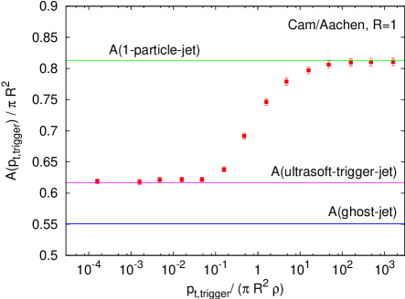
Figure 17 shows, as one expects, that there are two asymptotic regions. At large , the area tends to that of a jet with an infinitely hard particle, eq. (31). At small , it tends not to the pure ghost jet area, eq. (34), as one might naively expect, but rather to a value which can be predicted as
| (81) |
where is the distribution of the number of pure ghost jets with a given area, and corresponds to the solid curves depicted in figure 5. This equation can be understood in the following way: when the momentum of the trigger particle becomes negligible compared to that of the soft background, it does not influence the size of its own jet. However, the likelihood of the trigger particle being found in a soft-background jet is proportional to that soft-background jet’s area and one gets an extra factor of in the integrand of the numerator of eq. (81). One is able to use the pure-ghost-jet area distribution in eq. (81), because it coincides with that of soft background jets.
Figure 17 helps to illustrate the point that a diffuse background of particles such as pileup (represented here by the ghosts) provides an effective cutoff scale, below which a particle will not have any effect on the jet’s area. Numerically, the effective cutoff does indeed coincide with the soft-transverse momentum scale .
Appendix C Fluctuations of the active area
In this appendix, we derive the results eqs. (44)–(46) for the fluctuation coefficient in the case of active areas. This is slightly more technical than for passive areas as we also have to deal with averages over ghosts distributions. Let us briefly recall our notation: represents an average over perturbative emission, while is an average over ghosts ensembles. When a quantity is evaluated for a specific ghost ensemble , we will explicitly state so with notation of the form . From section 3 we have the implicit notation that a quantity specified without any mention of ghosts, such as is already averaged over ghost ensembles.
At order , the mean active area can then be written (using )
| (82) | |||||
| (83) | |||||
| (84) |
with
| (85) |
Here, we have taken into account both the corrections due to the radiation of a soft particle and the average over the distribution of the ghosts. Note that we have used the shorthand to represent eq. (11), , times , and that “” in eq. (82) represents all possible perturbative states.
For the corresponding fluctuations, the derivation goes along the same line
| (87) | |||||
Neglecting the terms proportional to , we can write , where
| (88) |
which for is the leading order result. We can also write
| (89) |
Using straightforward algebra one obtains
| (90) | |||||
| (91) | |||||
| (92) |
The second equality is a direct rewriting of the first. One gets to the last line by rearranging the different terms of the first one. The last two lines correspond exactly to eqs. (46) and (45) of section 3.3.
References
- [1] G. Sterman and S. Weinberg, Phys. Rev. Lett. 39 (1977) 1436.
- [2] for a review, see M. Dasgupta and G. P. Salam, J. Phys. G 30 (2004) R143 [arXiv:hep-ph/0312283].
- [3] M. H. Seymour, Nucl. Phys. B 513 (1998) 269 [arXiv:hep-ph/9707338]; A. Banfi, G. P. Salam and G. Zanderighi, JHEP 0408 (2004) 062 [arXiv:hep-ph/0407287].
- [4] R. Perez-Ramos, F. Arleo and B. Machet, arXiv:0712.2212 [hep-ph].
- [5] R. B. Appleby and M. H. Seymour, JHEP 0212 (2002) 063 [arXiv:hep-ph/0211426]; JHEP 0309 (2003) 056 [arXiv:hep-ph/0308086].
- [6] A. Banfi and M. Dasgupta, Phys. Lett. B 628 (2005) 49 [arXiv:hep-ph/0508159].
- [7] see e.g. N. Kidonakis and J. F. Owens, Phys. Rev. D 63 (2001) 054019 [hep-ph/0007268]; D. de Florian and W. Vogelsang, Phys. Rev. D 76 (2007) 074031 [arXiv:0704.1677 [hep-ph]].
- [8] R. Field [CDF Run II Collaboration],
- [9] J. M. Butterworth, J. R. Forshaw and M. H. Seymour, Z. Phys. C 72 (1996) 637 [arXiv:hep-ph/9601371].
- [10] M. Dasgupta, L. Magnea and G. P. Salam, arXiv:0712.3014 [hep-ph].
- [11] B. R. Webber, Phys. Lett. B 339 (1994) 148 [arXiv:hep-ph/9408222].
- [12] M. Dasgupta and G. P. Salam, J. Phys. G 30 (2004) R143 [arXiv:hep-ph/0312283].
- [13] D. de Florian and W. Vogelsang, Phys. Rev. D 76 (2007) 074031 [arXiv:0704.1677 [hep-ph]].
- [14] S. Catani, Y. L. Dokshitzer, M. H. Seymour and B. R. Webber, Nucl. Phys. B 406 (1993) 187 and refs. therein; S. D. Ellis and D. E. Soper, Phys. Rev. D 48 (1993) 3160 [hep-ph/9305266].
- [15] Y. L. Dokshitzer, G. D. Leder, S. Moretti and B. R. Webber, JHEP 9708, 001 (1997) [hep-ph/9707323]; M. Wobisch and T. Wengler, hep-ph/9907280.
- [16] G. P. Salam and G. Soyez, JHEP 0705 (2007) 086 [arXiv:0704.0292],
- [17] G. Corcella et al., arXiv:hep-ph/0210213.
- [18] T. Sjostrand et al., Comput. Phys. Commun. 135 (2001) 238 [hep-ph/0010017]; T. Sjostrand et al., hep-ph/0308153.
- [19] M. Cacciari and G. P. Salam, Phys. Lett. B 659 (2008) 119 [arXiv:0707.1378 [hep-ph]].
- [20] D. Y. Grigoriev, E. Jankowski and F. V. Tkachov, Phys. Rev. Lett. 91, 061801 (2003) [hep-ph/0301185]; Comput. Phys. Commun. 155, 42 (2003) [hep-ph/0301226].
- [21] L. Lonnblad, Z. Phys. C 58 (1993) 471.
- [22] G. C. Blazey et al., hep-ex/0005012.
- [23] M. Cacciari and G. P. Salam, Phys. Lett. B 641 (2006) 57 [hep-ph/0512210].
- [24] S. J. Fortune, Algorithmica (1987) 153–174.
- [25] A. Bhatti et al., Nucl. Instrum. Meth. A 566 (2006) 375 [arXiv:hep-ex/0510047].
- [26] G. P. Salam and D. Wicke, JHEP 0105, 061 (2001) [arXiv:hep-ph/0102343].
- [27] A. Banfi, G. Corcella and M. Dasgupta, JHEP 0703, 050 (2007) [arXiv:hep-ph/0612282].
- [28] T. Sjostrand and P. Z. Skands, Eur. Phys. J. C 39 (2005) 129 [arXiv:hep-ph/0408302].
- [29] M. Cacciari, G. P. Salam and G. Soyez, JHEP 0804 (2008) 063 [arXiv:0802.1189].
- [30] M. Dasgupta and G. P. Salam, Phys. Lett. B 512 (2001) 323 [arXiv:hep-ph/0104277]; JHEP 0203 (2002) 017 [arXiv:hep-ph/0203009].
- [31] A. Banfi, G. Marchesini and G. Smye, JHEP 0208, 006 (2002) [arXiv:hep-ph/0206076].