Reentrant magnetic ordering and percolation in a spin-crossover system

Abstract

Spin-crossover compounds, which are characterized by magnetic ions showing low-spin and high-spin states at thermally accessible energies, are ubiquitous in nature. We here focus on the effect of an exchange interaction on the collective properties for the case of non-magnetic low-spin ions, which applies to $\mathrm{Fe}^{2+}$ compounds. Monte Carlo simulations are used to study a three-dimensional spin-crossover model for the full parameter range from essentially pure high spin to essentially pure low spin. We find that as the low-spin state becomes more favorable, the Curie temperature drops, the universality class deviates from the three-dimensional Heisenberg class, and the transition eventually changes to first order. A heat-bath algorithm that grows or shrinks low-spin and high-spin domains is developed to handle the first-order transition. When the ground state has low spin, a reentrant magnetic transition is found in a broad parameter range. We also observe a percolation transition of the high spins, which branches off the first-order magnetic transition.

I Introduction

Spin-crossover materials are characterized by ions or atoms that can be in either a low-spin (LS) or a high-spin (HS) state. If the LS state is the ground state, they often show a crossover or phase transition to HS at higher temperatures, since the HS state has larger degeneracy and is thus entropically favored.CaS31 Spin-crossover systems include organometallic complexes,SCOrev ; BlP04 ; JSR07 organic radicals,FuA99 ; ICC02 Prussian Blue analogues,FMO95 ; SIF96 ; GRN00 ; BLE00 and other inorganic transition-metal salts.Co ; LVJ07 For example, a principal mineral in the Earth’s lower mantle is the spin-crossover compound $\mathrm{Mg}_{1-x}\mathrm{Fe}_{x}\mathrm{O}$.LVJ07

If the spins are carried by transition-metal ions, the energy difference between HS and LS is due to the interplay of crystal-field splitting of the d-levels and Hund’s rule coupling.SCOrev ; BlP04 For $\mathrm{Fe}^{2+}$ ions the LS state has spin quantum number $S=0$, whereas the HS state has $S=2$. Consequently, LS ions are essentially non-magnetic and effects due to the LS/HS transition are expected to be pronounced. These systems are related to diluted spin models,VMG02 ; dilute ; YRH04 ; PWD07 ; GoR07 but in spin-crossover systems the LS/HS degree of freedom is not quenched but dynamical.

Spin-crossover systems show interesting collective behavior, since they have two coupled degrees of freedom: the Heisenberg-type spin orientation and the Ising-type LS/HS degree of freedom. In one-dimensional systems, quantum fluctuations are important, in particular in the case of an antiferromagnetic exchange interaction.TiS05 ; Tim06 At zero temperature quantum effects in this case stabilize complex phases with magnetic unit-cell lengths of $3,5,7,\ldots$ lattice constants.TiS05

In this paper, we study a three-dimensional (3D) spin-crossover model including Heisenberg spins with isotropic exchange interaction. The LS state has spin $S=0$. This is the 3D version of the spin-crossover chain studied by Timm and Schollwöck.TiS05 We expect quantum fluctuations to be much weaker in 3D and employ a classical description. Nishino and coworkers NYM98 have studied a 3D model with Ising-type exchange, low spin $S=0$, and high spin $S=1/2$, i.e., two possible orientations of the high spins, employing mean-field theory and Monte Carlo (MC) simulations. Konishi et al.KTN06  have studied an Ising-type model for Prussian Blue analogues. Our model is different in that we describe Heisenberg spins, which are 3D unit vectors $\mathbf{S}_{i}$ interacting via an isotropic exchange interaction.

We perform MC simulations for the Heisenberg spin-crossover model on a simple cubic lattice. We are interested in the overall phase diagram, not in high-precision values for the transition temperature or critical exponents. In Sec. II we briefly introduce the model and discuss the simulation technique. In Sec. III we present and discuss our results, which are summarized in Sec. IV.

II Model and simulations

We are interested in 3D systems containing $\mathrm{Fe}^{2+}$ ions. Since the HS state has $S=2$ and the system is 3D, we expect quantum fluctuations to be relatively weak. We therefore start from the classical Hamiltonian

$$H=-V\sum_{\langle ij\rangle}\sigma_{i}\sigma_{j}-\Delta\sum_{i}\sigma_{i}\ -J\sum_{\langle ij\rangle}\mathbf{S}_{i}\cdot\mathbf{S}_{j},$$ (1)

where $\sigma_{i}$ equals $+1$ ($-1$) and $|\mathbf{S}_{i}|$ is zero (unity) for the LS (HS) state. We thus absorb the magnitude of the high spins into the exchange coupling $J$. $i$ runs over all sites of a simple cubic lattice, while $\langle ij\rangle$ denotes all nearest-neighbor bonds, counting each bond once. We can map the antiferromagnetic case $J<0$ onto the ferromagnetic case $J>0$ by flipping all spins on one sublattice. We thus restrict ourselves to $J\geq 0$ without loss of generality and express all energies in units of $J$. The coupling $V$ describes the affinity for equal LS/HS states on neighboring sites. This interaction is thought to be of mostly elastic origin.elastic ; NBY07 Finally, the Ising “magnetic field” $\Delta$ describes the on-site energy difference between HS and LS states. To be precise, the energy difference is $2\Delta$ and $\Delta>0$ favors a LS ground state.

The ground state is a ferromagnetic HS state for $\Delta/J<3/2$ and $V>\Delta/6-J/2$, a pure LS state for $\Delta/J>3/2$ and $V>-\Delta/6$, and a checkerboard LS/HS state for $V<\Delta/6-J/2$ and $V<-\Delta/6$. This is similar to the $T=0$ phase diagram for one-dimensional chains with ferromagnetic Ising exchange interaction.Tim06 We mostly concentrate on the case $V=0$.

We also need to specify the degeneracies of the LS and HS states. In the MC simulation these govern the attempt rates for LS-to-HS and HS-to-LS flips. Only the ratio of degeneracies is important because the physics is not affected by an overall constant factor in the partition function. For HS $S=2$ the underlying quantum system has a degeneracy factor of $g_{\mathrm{HS}}=5$ per site in the HS state and $g_{\mathrm{LS}}=1$ in the LS state. However, it is well known that the ratio $G\equiv g_{\mathrm{HS}}/g_{\mathrm{LS}}$ can be strongly enhanced due to softer vibrations in the HS state.BoK95 ; BCV95 ; YMK98 ; GKA00 ; NBY07

Our results apply to arbitrary degeneracies since one can absorb $G$ into an effective Ising magnetic fieldWaP70 ; Don78 ; NBY07

$$\Delta_{\mathrm{eff}}\equiv\Delta-\frac{T}{2}\,\ln G$$ (2)

(we take $k_{B}=1$). The simulations are therefore performed for $G=1$, i.e., with the same attempt rates for LS-to-HS and HS-to-LS flips. For specific systems, $\Delta$ is then replaced by $\Delta_{\mathrm{eff}}$.

We now turn to the MC simulations for this model. We simulate finite systems of size $L\times L\times L$ with periodic boundary conditions. The Heisenberg spins $\mathbf{S}_{i}$ are stored even for the LS sites, but the acceptance probabilities do not depend on them. We employ several different updates: (a) We use Wolff single-cluster updatesWol89 for the Heisenberg spins $\mathbf{S}_{i}$, but restricted to percolating clusters of high spins. This means that we choose a random site and, if it is in the HS state, grow a cluster to be flipped as in the original algorithm,Wol89 but only attempting to add neighboring HS sites. These cluster moves mostly avoid critical slowing down close to the second-order magnetic-ordering transition.

(b) We employ cluster updates of the LS/HS degree of freedom, which are also based on the Wolff algorithmWol89 and use a ghost spin to describe the local effective Ising magnetic field $\Delta$. The approach is similar to Rößler’s.Ros99 Since the Heisenberg spins are not updated, we absorb them into effective parameters for the Ising model of the $\sigma_{i}$. We first make the LS/HS dependence of the exchange term explicit by rewriting it as

$$-J\sum_{\langle ij\rangle}\frac{1-\sigma_{i}}{2}\,\frac{1-\sigma_{j}}{2}\,\mathbf{S}_{i}\cdot\mathbf{S}_{j}.$$ (3)

With this notation we can use $\mathbf{S}_{i}$ with unit magnitude regardless of whether a site is in the LS or HS state. Apart from a term that is independent of the $\sigma_{i}$, the Hamiltonian now reads

$$\tilde{H}=-\sum_{\langle ij\rangle}\tilde{V}_{ij}\,\sigma_{i}\sigma_{j}-\sum_{i}\tilde{\Delta}_{i}\,\sigma_{i}$$ (4)

with

$$\tilde{V}_{ij} \equiv V+\frac{J}{4}\,\mathbf{S}_{i}\cdot\mathbf{S}_{j},$$ (5)

$$\tilde{\Delta}_{i} \equiv \Delta_{\mathrm{eff}}-\frac{J}{4}\,\mathbf{S}_{i}\cdot\!\!\!\sum_{\mathrm{NN}\>j\>\mathrm{of}\>i}\!\mathbf{S}_{j},$$ (6)

where the last sum is over the nearest neighbors of $i$. The Hamiltonian (4) describes an Ising model with nonuniform interaction in a nonuniform field. We rewrite the external field as the interaction with a ghost spin $\sigma_{g}$, which couples to all sites $i$ with coupling $\tilde{V}_{ig}$. If we choose $\sigma_{g}=1$, we require $\tilde{V}_{ig}=\tilde{\Delta}_{i}$. The Hamiltonian then reads

$$\tilde{H}=-{\sum_{\langle ij\rangle}}^{\prime}\tilde{V}_{ij}\,\sigma_{i}\sigma_{j},$$ (7)

where the sum includes the ghost site. In the simulation, we chose a random site and try to add all bonds emanating from it. The probability for adding a bond from $i$ to $j$ is $P_{ij}=\max(0,1-e^{\Delta E/T})$, where $\Delta E$ is the change in energy according to Eq. (7). If $j$ is a normal lattice site, we really add it, but if it is the ghost site, we reject the entire cluster update. We then repeat these steps for all newly added sites. If we fail to add more sites but have not rejected the update, we flip all $\sigma_{i}$ on the cluster. This algorithm satisfies detailed balance.CzR97 ; Ros99

We also include (c) local spin rotations and (d) local LS/HS Ising spin flips within the Metropolis algorithm as a fallback when the cluster updates are inefficient. For a LS site, any spin rotation is accepted, since it does not cost any energy. We attempt approximately equal numbers of MC sweeps using (a)–(d), where one sweep is defined as touching every spin once on average.

The resulting routine is very robust, but suffers from one problem: In a relevant parameter range the magnetic transition is strongly first order. Standard methods to deal with first-order transitions such as multicanonical algorithmsBeN91 ; Mar98 or entropic samplingLee93 ; StH98 fail for an interesting reason: The low-temperature phase has a high HS fraction and ferromagnetic order, whereas the high-temperature phase shows a lower HS fraction and no magnetic order. In the high-temperature phase the Heisenberg spins are decoupled and typically randomly oriented. Starting from this phase, local LS/HS updates are inefficient because the HS phase is stabilized by the exchange interaction, which is zero for isolated high spins. However, LS/HS cluster updates also have very low probability of reaching the HS phase, since the random Heisenberg spins are energetically very unfavorable in the HS state. Thus we need updates that create large clusters of high spins and align them. It is difficult to do this efficiently while satisfying detailed balance.

Our algorithm uses a heat-bath technique that attempts to insert a layer of high spins which are well aligned with their neighbors. In detail, at any temperature we start by simulating two replicas of the system, which only differ in the starting configuration, which is pure HS with perfect ferromagnetic order and pure LS with random $\mathbf{S}_{i}$, respectively. If both phases are (meta-) stable and not very close together in configuration space, these replicas reach quasi-equilibrium in each phase, but do not overcome the barrier between them. We then take half of each replica and glue them together, thereby creating two phase boundaries. For reasons discussed below we cut in planes perpendicular to the $(111)$ direction.

The resulting system is then equilibrated using the updates (a)–(d) and one additional type (e) consisting of randomly selecting two layers $L_{1}$ and $L_{2}$ that are perpendicular to $(111)$, removing $L_{1}$, and shifting all layers between $L_{1}$ and $L_{2}$ (inclusive) by one primitive lattice vector $\hat{x}$. We then create new spins in layer $L_{2}$ using a heat-bath algorithm: At each site $i\in L_{2}$, $\sigma_{i}$ and $\mathbf{S}_{i}$ are randomly chosen with the proper Boltzmann probability distribution. The reason for choosing planes perpendicular to $(111)$ is that each site in $L_{2}$ only has neighbors that are not in $L_{2}$. Thus we can select each $(\sigma_{i},\mathbf{S}_{i})$ independently. If we had chosen layers perpendicular to $(100)$ we would have had to create a Boltzmann distribution of the entire layer. During the equilibration of the glued-together system, the updates (e) grow the more favorable phase and eventually remove the less favorable one.

Finally, we perform measurements for the equilibrated system. We wait for at least one MC sweep between measurements. Since the resulting time series is correlated, the errors are estimated using the blocking method.FlP89 The most important quantities we measure are the average square of the magnetization,

$$\langle\mathbf{M}^{2}\rangle\equiv\bigg{\langle}\frac{1}{L^{3}}\sum_{\mathrm{HS}\>i}\mathbf{S}_{i}\cdot\frac{1}{L^{3}}\sum_{\mathrm{HS}\>j}\mathbf{S}_{j}\bigg{\rangle},$$ (8)

where the sums are only over HS sites, the average fourth power of the magnetization, $\langle\mathbf{M}^{4}\rangle$, and the HS fraction

$$\gamma\equiv\bigg{\langle}\frac{1}{L^{3}}\sum_{i}\frac{1-\sigma_{i}}{2}\bigg{\rangle}.$$ (9)

Note that $\sigma_{i}=1$ ($-1$) for LS (HS).

The Binder cumulantBin81

$$C_{2}\equiv\frac{5}{2}-\frac{3}{2}\,\frac{\langle\mathbf{M}^{4}\rangle}{\langle\mathbf{M}^{2}\rangle^{2}}$$ (10)

is not as useful for the precision determination of the Curie temperature $T_{C}$ as for the pure Heisenberg model, since our model has two length scales, the correlation lengths $\xi$ of the Heisenberg spins $\mathbf{S}_{i}$ and $\xi_{\sigma}$ of the LS/HS degree of freedom $\sigma_{i}$. We expect $\xi_{\sigma}$ to be a continuous function of temperature through the magnetic transition like the HS fraction $\gamma$, as long as the transition is of second order. The Binder cumulant can be written as a scaling function $C_{2}=C_{2}(tL^{1/\nu},L/\xi_{\sigma})$, where $t\equiv(T-T_{C})/T_{C}$ and $\nu$ is the critical exponent of $\xi$. At $T=T_{C}$, we have $C_{2}=C_{2}(0,L/\xi_{\sigma}(T_{C}))$ so that the Binder cumulant does not become independent of system size. However, it is still true that the Binder cumulant approaches a step function for $L\to\infty$. For our definition (10) the step is from unity in the ordered phase to zero in the disordered phase. We can thus use $C_{2}=1/2$ as a criterion for $T_{C}$ that is correct in the limit of large $L$.

We also measure the fraction $P_{z}$ of configurations with a site-percolating HS cluster that wraps around the periodic boundaries in the z-direction, where the presence of this cluster is determined by a variant of the algorithm of Machta et al.MCL96 $P_{z}(T)$ curves for different system sizes $L$ are expected to intersect at the percolation transition in the limit of large $L$. Other definitions of the wrapping probability, e.g., wrapping in all directions, give the same result for the transition.NeZ01

III Results and discussion

In certain limiting cases, our model becomes either a pure Heisenberg model or a pure Ising model. We first discuss the Ising limit. $\Delta$ is a constant external field coupling to the Ising degree of freedom $\sigma_{i}$ and if we for the moment assume the Heisenberg spins to be frozen, they contribute nonuniform magnetic-field and coupling terms. The total Ising magnetic field is nonzero unless $\Delta=J=0$ and breaks the symmetry under $\sigma_{i}\to-\sigma_{i}$ and thus destroys the Ising critical point. The fact that the Ising magnetic field depends on the $\mathbf{S}_{i}$ and thus fluctuates does of course not restore the critical point.

Now consider the Heisenberg limit. The coupling to the LS/HS degree of freedom $\sigma_{i}$ does not break spin-rotation symmetry. If we freeze the $\sigma_{i}$ we have a diluted Heisenberg model, as noted above. The Harris criterion Har74 states that quenched disorder should be irrelevant for the critical behavior if the critical exponent $\nu$ of the correlation length satifies $\nu\geq 2/d$, where $d$ is the dimensionality of the system. For the pure Heisenberg model, $\nu=0.7112(5)$,CHP02 larger than $2/3$. Since disorder is thus irrelevant, the Heisenberg critical behavior should survive for a diluted system if it is not preempted by a first-order transition. This is indeed found in Ref. GoR07, .

However, the $\sigma_{i}$ are dynamical. Thus the Harris criterion does not apply and different critical behavior is possible—we return to this point below. Since spin-rotation symmetry is not broken explicitly by the coupling to $\sigma_{i}$, a spontaneous magnetic-ordering transition is still possible, though.

In addition, there can be a site-percolation transition of the high spins. Clearly, HS percolation is necessary but not sufficient for long-range magnetic order.

Figure 1: (Color online) Magnetization squared (solid curves) and HS fraction (dashed curves) for elastic interaction $V=0$ and various values of $\Delta/J$. For the magnetization curves, $\Delta$ increases from right to left. For $\Delta/J\geq 3/2$ the magnetization vanishes at all temperatures. The results have been obtained for system size $L=30$, $2000$ equilibration sweeps and at least $10000$ measurement sweeps. For several values of $\Delta/J$ the data points with error bars are shown.

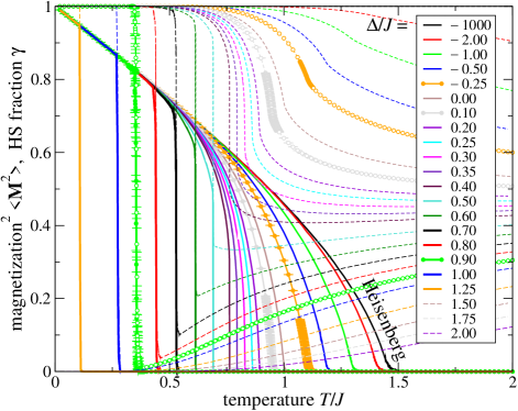
To prepare for the discussion of the phase diagram, we plot in Fig. 1 the magnetization squared, $\langle\mathbf{M}^{2}\rangle$, and the HS fraction $\gamma$ as functions of temperature $T$ for elastic interaction $V=0$ and various values of $\Delta/J$. Recall that $2\Delta$ is the bare energy difference between HS and LS states. We find four regimes:

For $\Delta/J\lesssim 0.30$, the magnetization vanishes at a second-order transition. The disordered phase above $T_{C}$ is predominantly HS. $\Delta\to-\infty$ corresponds to the pure Heisenberg model, where our results are consistent with $T_{C}/J\approx 1.457219(4)$ from high-precision MC simulations.CHP02 $T_{C}$ decreases with increasing $\Delta$.

For $0.30\lesssim\Delta/J\lesssim 0.55$, the magnetization vanishes at a first-order transition. The disordered phase is still mostly HS.

For $0.55\lesssim\Delta/J<3/2$, the transition is still of first order. The disordered phase immediately above $T_{C}$ is now mostly LS, but the HS fraction increases again with increasing temperature $T>T_{C}$.

For $\Delta/J\geq 3/2$ (exact value), there is no magnetic order at any temperature. The system is in a pure LS state at $T=0$ and the HS fraction increases smoothly with increasing temperature.

Figure 2: (Color online) (a) Phase diagram of the 3D Heisenberg spin-crossover model for elastic interaction $V=0$. The variables are (half) the bare LS/HS splitting in units of the exchange coupling, $\Delta/J$, and temperature. The solid curve with circles shows the magnetic transition. It approaches the pure Heisenberg limit (dotted line) for $\Delta\to-\infty$. Open (filled) circles represent a second-order (first-order) transition. The dotted curve with stars shows the HS percolation transition. Also shown are typical lines of constant $\Delta$ for ratios $G=g_{\mathrm{HS}}/g_{\mathrm{LS}}=1,10,100,1000$ of effective degeneracies for $\Delta/J=1.75$. For larger $G$, reentrant magnetic transitions are obvious. (b) Closeup of the intersection of magnetic and percolation transitions in (a).

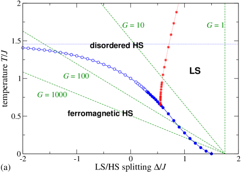
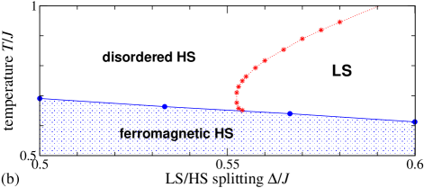
Figure 2 shows the phase diagram in the $(\Delta,T)$ plane for $V=0$. Since we are not interested in high-precision determination of transition temperatures, we employ the following criteria to map out the transitions: $T_{C}$ is estimated from the Binder commulant $C_{2}=1/2$ found by bisection for $L=30$ with $20000$ equilibration sweeps and $2^{17}=131072$ measurement sweeps for each data point. (For $\Delta/J=0.25$ the resulting $T_{C}$ is indistinguishable on the scale of Fig. 2(a) from the one obtained below from finite-size scaling.) The temperature of the percolation transition is estimated from the intersection of $P_{z}(T)$ for $L=30$ and $L=40$ found by bisection with $20000$ equilibration sweeps and $131072$ measurement sweeps.

The phase diagram Fig. 2(a) shows that $T_{C}$ decreases smoothly with increasing $\Delta$. Note that $T_{C}$ is already significantly reduced for $\Delta\lesssim 0$, where the ground state of an uncoupled site is still HS. The low-temperature phase remains ferromagnetically ordered for small positive $\Delta$ due to the exchange interaction, which favors HS. The character of the magnetic transition changes from second order to first order at $\Delta/J=0.313(5)$ and $T_{C}$ approaches zero continuously at $\Delta/J=3/2$.

The HS percolation transition intersects with the magnetic transition where the latter is of first order. It then coincides with the first-order transition down to the point $\Delta/J=3/2$, $T_{C}=0$. The intersection point does not have any special properties; the percolation transition continues for the undercooled magnetically disordered state (not shown). It is seen that on approaching the magnetic transition, the percolation transition curves away towards the LS phase. This shows that the HS phase is favored even though there is no ferromagnetic order yet. This can be attributed to short-range ferromagnetic correlations. The fluctuations responsible for these correlations are relatively strong although the magnetic transition is of first order, since the parameters are close to the endpoint of the first-order line. Figure 2(b) shows that the percolation transition is reentrant as a function of temperature in the vicinity of $\Delta/J=0.553$.

Recall that arbitrary ratios $G=g_{\mathrm{HS}}/g_{\mathrm{LS}}$ of effective degeneracies can be incorporated by replacing $\Delta$ by $\Delta_{\mathrm{eff}}=\Delta-(T/2)\,\ln G$. Curves of fixed $\Delta$ in the $(\Delta_{\mathrm{eff}},T)$ phase diagram are straight lines of slope $-2/\ln G$. Since $G>1$ (and often $G\gg 1$, Ref. BCV95, ), the slope is negative. Examples are shown in Fig. 2(a). It is clear that for not too small $G$ this leads to reentrant magnetic transitions: With increasing temperature the system goes from paramagnetic (usually LS), to ferromagnetic HS, to paramagnetic (usually HS). What happens physically is that the increasing temperature entropically favors HS until the free energy of the ferromagnetic HS state becomes lower than that of the LS state. At higher temperature thermal fluctuations eventually destroy magnetic order, but HS remains entropically favored.

Figure 3: (Color online) Magnetization squared (solid curves) and HS fraction (dashed curves) for elastic interaction $V/J=0.25$ and various values of $\Delta/J$. For the magnetization curves, $\Delta$ increases from right to left. For $\Delta/J\geq 3/2$ the magnetization vanishes at all temperatures. The results have been obtained for system size $L=30$, $2000$ equilibration sweeps and at least $10000$ measurement sweeps. The dotted curve shows $\langle\mathbf{M}^{2}\rangle$ for the Heisenberg case.

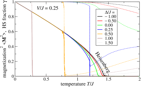
We briefly consider the case of $V\neq 0$. Figure 3 shows the magnetization squared and the HS fraction for $V/J=0.25$. Positive $V$ favors neighboring sites both in the LS or both in the HS state, thereby stabilizing phases with HS fractions $\gamma\approx 0$ or $\gamma\approx 1$. We expect this to favor first-order magnetic transitions accompanied by a large jump in $\gamma$, which is indeed seen in Fig. 3. For example, for $\Delta/J=0.25$ the transition is now of first order, whereas it is of second order for $V=0$, cf. Fig. 1. In addition, at the same $\Delta/J$, positive $V$ stabilizes the ferromagnetic HS phase, increasing $T_{C}$. However, the $T=0$ transition is at $\Delta/J=3/2$ for all $V/J\geq-1/4$.

Figure 4: (Color online) Magnetization squared (solid curves) and HS fraction (dashed curves) for elastic interaction $V/J=-0.25$ and various values of $\Delta/J$. For the magnetization curves, $\Delta$ increases from right to left. For $\Delta/J\geq 3/2$ the magnetization vanishes at all temperatures. This is a special point in the $T=0$ phase diagram where ferromagnetic HS, pure LS, and checkerboard phases meet. The results have been obtained for system size $L=30$, at least $2000$ equilibration sweeps and at least $10000$ measurement sweeps. For two values of $\Delta/J$ the data points with error bars are shown. The dotted curve shows $\langle\mathbf{M}^{2}\rangle$ for the Heisenberg case.

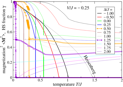
Figure 4 shows the magnetization squared and the HS fraction for $V/J=-0.25$. Negative $V$ favors neighboring sites in different LS and HS states. In fact for $V/J<-1/4$ the $T=0$ phase diagram contains a checkerboard LS/HS phase at $\Delta/J$ around $3/2$. At the point $V/J=-1/4$, $\Delta/J=3/2$ three phases (ferromagnetic HS, pure LS, and checkerboard) meet.

We find two phase transitions for intermediate values of $\Delta/J$: The HS fraction $\gamma$ shows a sharp kink above $T_{C}$. We also note that the HS fraction $\gamma$ is close to $1/2$ for $T\gtrsim T_{C}$, consistent with checkerboard order of the LS/HS degree of freedom. An analysis of the average staggered Ising order parameter, $\langle|L^{-3}\,\sum_{i}(-1)^{i}\sigma_{i}|\rangle$ (not shown) finds long-range checkerboard order in the intervening phase. This phase thus appears at finite temperatures for $V/J=-0.25$, although at $T=0$ it is absent except at $\Delta/J=3/2$, as noted.

In addition, first-order transitions are again favored compared to $V=0$: For $\Delta/J=0.25$ the transition is of first order for $V/J=-0.25$ and $0.25$ but not for $V=0$. Furthermore, $T_{C}$ for the same $\Delta/J$ is significantly reduced compared to $V\geq 0$, since neighboring LS/HS pairs are of course unfavorable for magnetic order.

Figure 5: (Color online) Scaled magnetization squared, $\langle\mathbf{M}^{2}\rangle\,L^{2\beta/\nu}$, vs. scaled temperature, $t\,L^{1/\nu}$, for $V=0$, $\Delta/J=0.25$ for system sizes $L=25,30,40,50$. The results have been obtained using at least $2000$ equilibration sweeps and $262144$ measurement sweeps. Inset: The same quantities with the same value of $T_{C}$ scaled with the exponents $\beta$, $\nu$ of the pure Heisenberg model.

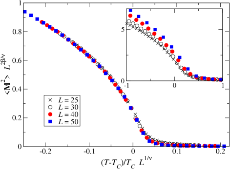
We next discuss the nature of the magnetic transition in some more detail. As noted above, the Harris criterionHar74 is not applicable to our model. It is thus reasonable to ask whether the dynamical dilution changes the universality class where the transition is of second order. To answer this question, we perform finite-size scaling for the case of $\Delta/J=0.25$, for which the transition is of second order, but close to the end point of the first-order line, see Figs. 1 and 2(a). The magnetization squared close to the transition should scale like $\langle\mathbf{M}^{2}\rangle\,L^{2\beta/\nu}\sim\Phi\!\left(t\,L^{1/\nu}\right)$ with $t\equiv(T-T_{C})/T_{C}$, where $\Phi$ is a universal function. A least-square fit for system sizes $L=40$ and $L=50$ yields $T_{C}/J=0.8604(2)$, $\beta=0.26(2)$, and $\nu=1.30(8)$. The errors are the ones incurred by the least-square fit, which are much larger than the statistical errors of $\langle\mathbf{M}^{2}\rangle$. The scaled magnetization squared is plotted vs. the scaled temperature for sizes $L=25,30,40,50$ in Fig. 5. It is apparent that corrections to scaling are relatively large. Nevertheless, the behavior is clearly inconsistent with the 3D Heisenberg exponents $\beta=0.3689(3)$ and $\nu=0.7112(5)$.CHP02 The inset in Fig. 5 shows that the scaling fails for Heisenberg critical exponents. Since Figs. 1 and 2 do not show any qualitative change in the second-order magnetic transition as a function of $\Delta$, we conjecture that the critical exponents smoothly approach the 3D Heisenberg limit for $\Delta\to-\infty$.

Figure 6: (Color online) Probabilities for finding a spanning HS cluster in the z-direction (upper panels) and HS fraction (lower panels) as functions of temperature for (a) $\Delta/J=0.60$ and (b) $\Delta/J=0.75$ and system sizes $L=25,30,40,50$. The horizontal dashed line indicates the critical percolating HS fraction in the absence of correlations. The vertical dashed lines mark the positions of the percolation transitions.

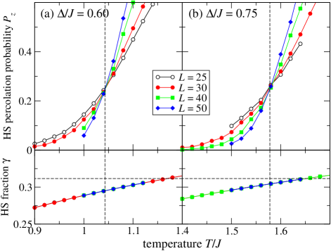
Finally, we turn to the HS percolation transition. For uncorrelated $\sigma_{i}$, the transition would take place at a HS fraction of $\gamma=\gamma_{p0}=0.3116081(21)$.BFM99 In our case, there are short-range correlations between the $\sigma_{i}$, even for $V=0$, due to the exchange interaction $J$, which favors high spins at nearest-neighbor sites. We have seen that these correlations shift the percolation transition towards larger $\Delta$. Thus there is no reason to expect the HS percolation transition to take place at $\gamma=\gamma_{p0}$. Figure 6 shows the probability $P_{z}$ of finding a HS cluster spanning the system in the z-direction as a function of temperature for two values of $\Delta$ and several system sizes. The crossing of $P_{z}$ curves indicates the percolation transition.MCL96 The lower panels show the HS fraction $\gamma$ and also the value $\gamma_{p0}$. The HS fraction at the percolation transition, $\gamma_{p}$, is inconsistent with $\gamma_{p0}$: For $\Delta/J=0.75$ we find $\gamma_{p}\approx 0.304$ and for $\Delta/J=0.6$, closer to $T_{C}$, $\gamma_{p}\approx 0.295$. Thus the high spins percolate at a lower HS fraction than they would for a random distribution, as expected for positive correlations between neighboring high spins.

IV Summary

We have performed MC simulations for a 3D spin-crossover model with Heisenberg exchange interaction and spin $S=0$ in the LS state, as realized in $\mathrm{Fe}^{2+}$ compounds. A full range of onsite energy differences $2\Delta$ between HS and LS has been explored, from values strongly favoring HS to values strongly favoring LS. We have focused on the case of negligible elastic interaction. The main results are the following: The Curie temperature is significantly reduced already on the HS side ($\Delta<0$), but initially remains nonzero on the LS side ($\Delta>0$) due to the exchange interaction $J$, which favors HS. As $\Delta$ increases further, the character of the transition changes from second to first order and $T_{C}$ decreases continuously until it reaches zero at a specific value of $\Delta$. A MC method involving growing and shrinking LS and HS domains has been introduced to tackle the first-order transition.

Where the magnetic transition is of second order, it is not in the 3D Heisenberg universality class, at least close to the onset of first-order transitions. The system also shows a HS site-percolation transition, which intersects the first-order magnetic transition. Its position is affected by short-range magnetic correlations. They also lead to a smaller HS fraction $\gamma$ at the percolation transition than for a random percolation model.

For the realistic case of a LS ground state and an excited HS state with much larger degeneracy, we find reentrant magnetic transitions. Increasing temperature entropically favors HS, which stabilizes ferromagnetic order in an intermediate temperature range.