Variability of the proton-to-electron mass ratio on cosmological scales
Abstract
The search for a possible variation of fundamental physical constants is newsworthy more than ever. A multitude of methods were developed. So far the only seemingly significant indication of a cosmological variation exists for the proton-to-electron mass ratio as stated by Reinhold et al. Reinhold06 . The measured indication of variation is based on the combined analysis of H2 absorption systems in the spectra of Q0405-443 and Q0347-383 at and , respectively. The high resolution data of the latter is reanalyzed in this work to examine the influence of different fitting procedures and further potential nonconformities. This analysis cannot reproduce the significance achieved by the previous works.
1 Introduction
Contemporary theories of fundamental interactions, particularly those subsumed
as string theories allow for all kinds of variations of fundamental constants in
the course
of the evolution of the universe. Variations of the coupling constants of
strong and electroweak interactions would affect the masses of elementary
particles dependent on the model for the expanding universe.
It is up to cosmology to achieve first
estimates and constraints of possible variations on large scale since laboratory
experiments lack the spatial or temporal coverage.
A recent analysis of HE 0515-4414 by Chand et al. Chand06 and Molaro et al. Molaro07 yielded a result for the fine structure constant that is in
good agreement with
no variation at the current level of accuracy. However there are
results indicating a variation in or not yet fully controlled
systematics (Murphy et al. Murphy04 , Levshakov et al. Levshakov07 ).
A measured trend of positive variation in the proton-to-electron mass
ratio by Ivanchik et al. Ivanchik05 and a later refinement to
Reinhold06 launched numerous
theories with
different scenarios to interpret the new data. The subject is still under heavy
debate and confirmation of the results and methods is required.
2 Detecting via molecular hydrogen
The latest measured value of the proton-to-electron mass ratio is Mohr05 . The precision reached by today’s laboratory experiments rules out considerable variation of on short time scales but cannot yet exclude a change over cosmological timescales on the order of years. Additionally the possibility of different proton-to-electron mass ratios in widely separated regions of the universe cannot be rejected. The method to constrain a possible variation of as applied in this work was first suggested by Thompson Thompson75 . Electronic, vibrational, and rotational excitations of a diatomic molecule depend differently on its reduced mass . To a first approximation, these energies are proportional to , , , respectively. Hence each transition has an individual sensitivity to a possible change in that reduced mass. This can be expressed by a sensitivity coefficient.
| (1) |
The calculations of were recently refined by Reinhold et al. Reinhold06 . In first order they can be expressed by the Dunham coefficients of the ground and excited states. With , Equation 1 leads to:
| (2) |
The computations for the energies of the excited and ground state, and , respectively are the same as for the energy levels of H2. Starting with the BOA based on the semiempirical approach the energy levels can be expressed by the Dunham formula
| (3) |
However, the Dunham coefficients cannot be calculated directly from the level energies due to strong mutual interaction between the excited states as well as avoided rotational transitions between nearby vibrational levels. For the first time the more complex non-BOA effects are taken into account in the work of Reinhold et al. Reinhold06 . Their recent precise laboratory measurements of the level energies of molecular hydrogen allowed for a reliable enhancement of the BOA approximation. The influence of the inclusion of the Bohr shift and adiabatic corrections is shown in Figure 1 (right) in percentage compared to prior sensitivity coefficients Varshalovich95 .
 |
 |
2.1 Distinguish cosmological redshifts from variation of
With from Equation 1, the rest frame wavelengths are related to those in the quasar absorption system via
| (4) |
with as the redshift of the absorbing system. This can be expressed in terms of the individual redshift of each measured H2 component:
| (5) |
According to Equation 5 the redshift of each H2 feature can be distinguished between the intrinsic redshift of the absorber and an additional component due to a possible variation in . Equation 5 describes a simple linear equation with a gradient of
| (6) |
A linear regression of the redshift of each H2 line and its individual sensitivity coefficient will yield the redshift of the absorbing DLA system and during the epoch between and today. It is worth noting that in the case of non-zero variation the redshift of the absorber is not identical to the mean redshift of all observed lines as can be derived from Equation 5.
3 Observations
The source (Q0347-383) of the analyzed spectrum is a bright
quasi-stellar radio object
(QSO) with a visual magnitude of at a redshift of
Maoz93 .
The precise position dated to 2000 as stated in the fifth fundamental catalogue
is 03h 49m 43.68s, -38∘10’ 31.3”.
The Quasar absorption line spectra were obtained with the Ultraviolet and
Visual Echelle Spectrograph (UVES) at the Very
Large Telescope (VLT) of the European Southern Observatory (ESO) in Paranal,
Chile.
The slit was 0.8 arcsec wide resulting in a spectral resolution of
53.000 over the wavelength range 3300Å – 4500Å.
The average seeing during observation was about 1.2 arcsec. Before and after the
exposures for each night, Thorium-Argon calibration data were taken.
An overall of nine spectra were recorded with an exposure time of 4500 seconds
each between January 8th and January 10th 2002 for the ESO program
68.A-0106(A). All spectra were taken with grating 430 and the blue
“Pavarotti”-CCD with 2x2 binning. Later on the data were reduced manually by
Mirka Dessauges-Zavadsky from Geneva Observatory in Jan 2004 to achieve
maximum accuracy. The ESO Ambient Conditions
Database111http://archive.eso.org/eso/ambient-database.html includes
measurements of the environmental parameters at the Paranal ESO observatory and
shows no significant changes in temperatures during or inbetween the
exposures that could lead to shifts between the separate observations.
The reduced data used here is identical to the one in
Ivanchik05 and Reinhold06 .
4 Data analysis
The nine separate spectra are coadded only to identify H2 lines with a higher signal-to-noise ratio. The fitting is carried out simultaneously on the separate spectra to avoid influences of slight shifts between the datasets. The observed spectral range of the data covers over 80 H2 lines of which after careful selection and avoidance of blends only 39 are taken into account for the analysis. The H2 lines are mostly noticeable by their narrow line profiles and generally low equivalent width. The observed spectrum has an instrumental resolution of 5.6 . That corresponds to a temperature of more than 4000K for Doppler broadened H2 lines. A lower excitation temperature is to be expected for intergalactic molecular Hydrogen. The observed width of the H2 features can thus be expected to be given by the spectral resolution.
4.1 Fitting of H2 features
The selected and verified H2 lines are fitted with an evolutionary fitting algorithm Quast05 . Due to the nature of DLA systems the continuum is heavily contaminated. The background is determined over a given range of the line feature and fitted with a polynomial. That range is selected individually for each line by eye to have the best compromise between a clean continuum and the number of pixels contributing to it. The grade of the polynomial is manually selected to match the continuum flux. In some cases an additional line is fitted along with the H2 component to have a better fit to the flux. For those cases the true continuum is fitted via a linear function. In cases of a continuum flux with apparent influences of broad Lyman features or general contamination, a parabolic or cubic function is used to fit the background to the observed flux. See Figure 2 of L3R3 and L6R3 for an exemplar of a parabolic fit.
This approach – however necessary – is highly critical. The applied rectification of the flux may have an impact on the fitted central position of the line feature. For the analysis in Reinhold06 and Ivanchik05 the estimated background is constructed manually.
 |
 |
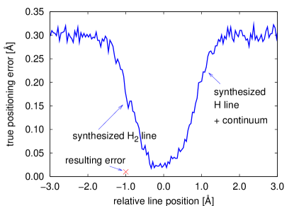
To ascertain the validity of this approach a series of fits for simulated spectra is carried out. A spectrum of a hypothetical H2 feature on the wing of a broad almost saturated Hi absorption feature is synthesized. Its relative position to the center of the Hi feature is altered to cover the full area of influence of the dominant atomic hydrogen feature. For each constellation 100 spectra are synthesized and fitted. Figure 3 (left) shows an example setup. For the given position of the H2 feature the resulting error in determining the center of the H2 absorption feature can be computed by the difference of the input to the artificially generated spectrum and the output of the fitting algorithm. On the right panel of Figure 3 the results of a full run of 10,000 fits are plotted.
 |
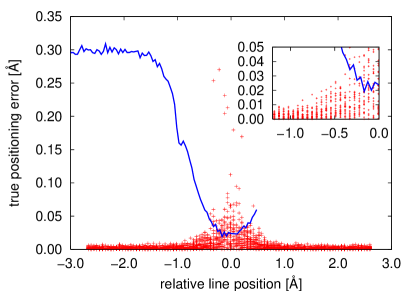 |
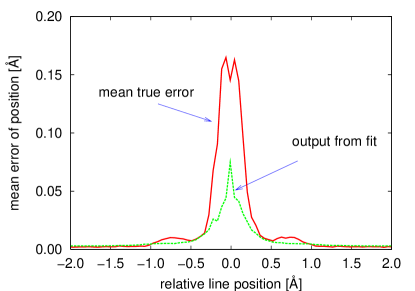
Figure 4 illustrates the averaged computed absolute error and the error as ascertained by the fitting algorithm. To evaluate the accuracy of a polynomial continuum fit, two separate runs are carried out. One with a parabolic continuum fit (left panel) and one with a linear continuum but a second absorption line (in this case the broad Hi line) as free parameter to match the observed flux (right panel). The latter representing the true physical conditions but not being feasible on heavily contaminated continua.
 |
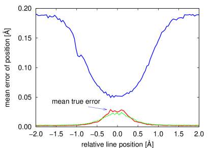 |
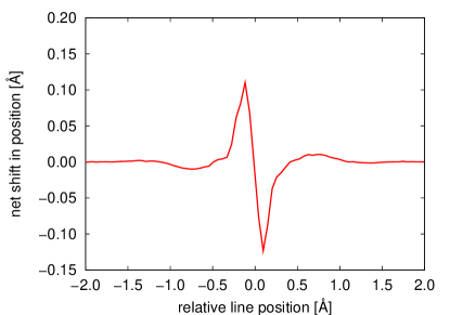
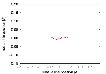
The results indicate that modelling the pseudo continuum with a polynomial is valid when being performed carefully with respect to the underlying absorption. The error rises dramtically for positions near the center of the Hi absorption which is understandable due to the low equivalent width of the H2 feature. However in the case of the polynomial continuum fit this effect has greater influence. Furthermore the application of the polynomial fit to the continuum and accordingly the rectification of the flux introduces a net shift in the determination of the as seen in Figure 5. An error that may not average out for low statistics.
 |
 |
4.2 Selection of lines
The strong contamination of the observed spectrum forces us to find a balance between a sufficiently high number of H2 features taken into account for better statistics and the quality of the surrounding continuum. An independent selection via curve of growth analysis yields the same group of H2 lines as used in Reinhold06 and Ivanchik05 .
5 Results

All 39 lines are fitted and a corresponding redshift is derived. The
measured redshifts with their obtained standard deviations are not consistent
with a single mean redshift at the level.
Accordant to the method described in Section 2 the measured
redshifts are tested for a possible correlation with the individual sensitivity
coefficients. Figure 6 shows the resulting plot. The dotted line
represents a preliminary linear fit to the data.
The redshift of the absorber does not correspond to the mean
redshift, but can be ascertained by the point of zero sensitivity towards
possible -variation, since at this point the measured redshift equals the
cosmological redshift (see Eq. 5). The ordinate is given
in relative redshift with respect to the absorber
.
The linear fit corresponding to is
achieved by a linear regression without taking into account the individual
estimated errors in the redshift to allow for a comparison with the results of
Reinhold et al. Reinhold06 who measured
with the method of an unweighted fit but based on a merged dataset of two
quasars at different redshifts.
The argumentation behind an unweighted fit is that the dispersion of the
experimental points then characterizes the true statistical errors. At a 95%
confidence level this results gives a constraint of the variation to
. However, a straight
forward linear fit to the data turns out to be inappropriate.
Figure 7 illustrates the – relation for all
three observed rotational levels combined (top left) and each of them
separately (top right and bottom). Evidently only the first
rotational level shows an apparent correlation between redshift and
sensitivity coefficients .
Table 2 gives the mean redshifts for each
corresponding rotational level. It is worth noting that the deviation
from
the mean value is smaller than the 2 level of the mean
estimated error .
The number of lines is too low to make significant statistical claims.
However, the Pearson product-moment correlation coefficient (equivalent to dividing the covariance between two variables by the product of their standard deviations) indicates only a very weak correlation of the data. Apparently only the first rotational level contributes to a positive linear correlation at all (see Table 1). A closer examination of the first rotational level (see Figure 7 upper right) by eye shows that the positive gradient of the linear regression seems to evolve only by the rightmost seven data points. This impression can be confirmed by a correlation test for all data points except those seven lines with . Table 1 lists the correlation coefficient of this subset as . A result quite consistent with no correlation at all (see Fig.8). However, seven data points represent a considerable subset of the total of 39 lines. The seven lines (namely L7R1, L8R1, L9R1, L9P1, L10P1, L13R1, L14R1) evidently have a sensitivity coefficient of in common, they also emerge from high energy transitions. As can be seen from the line identifiers, the seven lines in question all arise from high vibrational levels in the Lyman band. This matches fully with the range where the sensitivity coefficients deviate the most from the Born-Oppenheimer-approximated calculations Reinhold06 .
| rotational level | r | data points |
|---|---|---|
| 1 | 0.29 | 18 |
| 2 | -0.16 | 10 |
| 3 | -0.62 | 11 |
| all | 0.24 | 39 |
| subset | -0.08 | 32 |
5.1 Goodness of fit
To quantify the - correlation further a Spearman rank-order correlation coefficient is calculated. It is a non-parametric measure of correlation, i.e., it assesses how well an arbitrary monotonic function could describe the relationship between two variables without making any assumptions about the frequency distribution of the variables. Unlike the Pearson product-moment correlation coefficient, it does not require the assumption that the relationship between the variables is linear nor does it require the variables to be measured on interval scales. Furthermore it allows to determine the significance of a non-zero correlation. Instead of measured values merely their ranks are compared. The analysis gives coefficients of for the full set of lines and for the subset of 32 lines (see Figure 8). The latter being not significant at the 99.9% level (i.e., in only 0.1% of all cases a non-zero correlation can be deduced from a correlation coefficient of ) thus in full agreement with no correlation. The obtained Spearman rank-order correlation coefficients occur in case of zero-correlation with probabilities of and , respectively.
The goodness of fit states how well a statistical model fits a set of observations in contrast to a general of a fit which only states the confidence of the fit. The based fit allows for a statement on the quality or rather the likelihood of a fit in respect to the model. Due to the simplicity of the assumed model (see Eq.5) the relation between measured redshift and computed sensitivity coefficient is stringently linear in case of variation. In case of no variation the gradient would be zero but still fit the assumed linear model. As a consequence, any result must be consistent with a linear correlation between and independently of a possible variation. The performed simulations of linefits indicated that the fit error on the observed wavelength for each line and thus the error in the relative redshift as estimated by the fitting programme are reasonable. This, of course, depends also on the accuracy of the errors given in the observed data. The correctness of the errors in the spectral data can be crudely tested by the value of a reasonably good fit. However, the is influenced by the trueness of the error as well as the accuracy of the model. The mean value of all 351 fitted lines (39 lines in 9 spectra) is with a more descriptive median of exactly . The mean is expected to lie above the median due to the fact that for some absorption features the model of a single component is evidently wrong and thus the flux is not fitted by the model for the whole evaluated range.
The goodness of fit for the fitted linear relation gives a likelihood of the fit of . This strongly indicates that the errors in general are underestimated. A lowered likelihood can also emerge from measurement errors that are strongly non-normally distributed. The simulations with synthesized data, however, did show that the errors of the fit are in good agreement with a normal distribution for the lines selected. The validity of the assumed model is convincing and the errors of the fitted redshifts appear to be systematically underestimated. The fitted linear relation is not at all consistent with the observed data and the adopted error simply reflects the statistically best solution without considering consistency with the data. However, the likelihood of the fit scales rather strongly with the errors of the observed redshift. Assuming the greatest uncertainty in the measured redshifts despite the evidently accurate output of the fitting program, the errors given for the redshifts were scaled by a constant factor. A scaling by a factor of two results in a likelihood of the fitted data of about which would be acceptable, though still being low.
 |
 |
 |
 |
| J | |||
|---|---|---|---|
| 1 | 3.0249022 | 3.8 | 1.9 |
| 2 | 3.0248982 | 5.3 | 3.8 |
| 3 | 3.0248984 | 5.7 | 3.2 |

Note, that for this analysis a constant shift or offset in wavelength calibration has no impact on the deduced correlation. Only differential shifts would influence the outcome of the analysis.
6 Conclusions
Asking for self consistency in the result, brings down the significance of the measurement of a possible variation to at once. Rejecting the subset of seven lines of a single rotational level from the dataset leads to no correlation at all, since the correlation is already very weak as discussed above. A linear fit is no longer reasonable. A detection of a positive variation of is caused solely from transitions for which and in the upper state, i.e., a range of transitions with significant non-BOA effects as reflected in the large changes in recently calculated or for these vibrational bands. The discrepancy of the observed redshifts and their errors with the basic model of points out yet not fully understood systematic errors. Possible reasons for the scatter in the redshift of several can be that a resolution of 53.000 is not sufficient for accurate linefits of unresolved H2 features and thus the positioning error is systematically underestimated.
A possible cause for differences in measured redshifts between the excitation levels can also be a spatially separation between the points of origin. The nature of DLAs is not yet fully understood and subject to several inconsistencies. Recent simulations indicate that molecular hydrogen is distributed highly inhomogeneous and clumpy Hirashita03 . Despite the successful refinement of transition frequencies for H2 their accuracy for intergalactic physical conditions requires further verification. The yet unknown origin of the scatter of measures redshift in this work and others demands great care in future analysis and renders the gain in significance by combining data of several systems questionable. It would rather indicate the need for more careful selection of analyzed features, an in-depth study of the according transition wavelengths as well as a high precision reduction of the observed data in all particular steps (i.e. the data acquisition itself, wavelength calibration across several orders, vacuum correction). The level at which possible variations are investigated today sets high demands on all steps involved.
A possible variation of the proton-to-electron mass ratio cannot be confirmed. Furthermore the inconsistency of the data and the errors with respect to the scattering of the observed redshifts give reason to be more careful in formulating constraints as well.
The resulting constraint of this work at the 95% level is over the period of 11.5 Gyr, or a maximum change of by yr-1 for the hypothetical case of linear variation in time. The light travel time of 11.496 Gyr for corresponds to the cosmological parameters .
7 Acknowledgements
We are thankful for the support from the Collaborative Research Centre 676 and for helpful comments by S. A. Levshakov, P. Petitjean and R. I. Thompson.
References
- (1) E. Reinhold et al., Physical Review Letters 96, (2006)
- (2) H. Chand et al., A&A 451, (2006) 45-56
- (3) P. Molaro et al., A&A 712, (2007)
- (4) A. Ivanchik et al., A&A 440, (2005) 45-52
- (5) M. T. Murphy, V. V. Flambaum, J. K. Webb et al., Lecture Notes Phys. 648, (2004) 131
- (6) S. A. Levshakov, P. Molaro, S. Lopez et al., A&A 466, (2007) 1077
- (7) R. I. Thompson, Astrophysical Letters 13, (1975) 3,4
- (8) P. J. Mohr and B. N. Taylor, Reviews of Modern Physics 77, (2005) 1-107
- (9) D. A. Varshalovich and A. Y. Potekhin, Space Science Reviews 74, (1995) 259-268
- (10) D. Maoz et al., ApJ 409, (1993) 28-41
- (11) R. Quast, R. Baade and D. Reimers, A&A 431, (2005) 1167-1175
- (12) H. Hirashita, A. Ferrara, K. Wada, P. Richter, MNRAS 18, (2003) 341