Average-Case Analysis of
Online Topological Ordering

Abstract

Many applications like pointer analysis and incremental compilation require maintaining a topological ordering of the nodes of a directed acyclic graph (DAG) under dynamic updates. All known algorithms for this problem are either only analyzed for worst-case insertion sequences or only evaluated experimentally on random DAGs. We present the first average-case analysis of online topological ordering algorithms. We prove an expected runtime of ${\cal O}(n^{2}\,\operatorname{polylog}(n))$ under insertion of the edges of a complete DAG in a random order for the algorithms of Alpern et al. (SODA, 1990), Katriel and Bodlaender (TALG, 2006), and Pearce and Kelly (JEA, 2006). This is much less than the best known worst-case bound ${\cal O}(n^{2.75})$ for this problem.

1 Introduction

There has been a growing interest in dynamic graph algorithms over the last two decades due to their applications in a variety of contexts including operating systems, information systems, network management, assembly planning, VLSI design and graphical applications. Typical dynamic graph algorithms maintain a certain property (e. g., connectivity information) of a graph that changes (a new edge inserted or an existing edge deleted) dynamically over time. An algorithm or a problem is called fully dynamic if both edge insertions and deletions are allowed, and it is called partially dynamic if only one (either only insertion or only deletion) is allowed. If only insertions are allowed, the partially dynamic algorithm is called incremental; if only deletions are allowed, it is called decremental. While a number of fully dynamic algorithms have been obtained for various properties on undirected graphs (see [10] and references therein), the design and analysis of fully dynamic algorithms for directed graphs has turned out to be much harder (e. g., [25, 26, 24, 13]). Much of the research on directed graphs is therefore concentrated on the design of partially dynamic algorithms instead (e. g., [7, 3, 14]). In this paper, we focus on the analysis of algorithms for maintaining a topological ordering of directed graphs in an incremental setting.

A topological order $T$ of a directed graph $G=(V,E)$ (with $n:=|V|$ and $m:=|E|$) is a linear ordering of its nodes such that for all directed paths from $x\in V$ to $y\in V$ ($x\neq y$), it holds that $T(x)<T(y)$. A directed graph has a topological ordering if and only if it is acyclic. There are well-known algorithms for computing the topological ordering of a directed acyclic graph (DAG) in ${\cal O}(m+n)$ time in an offline setting (see e. g. [8]). In a fully dynamic setting, each time an edge is added or deleted from the DAG, we are required to update the bijective mapping $T$. In the online/incremental variant of this problem, the edges of the DAG are not known in advance but are inserted one at a time (no deletions allowed). As the topological order remains valid when removing edges, most algorithms for online topological ordering can also handle the fully dynamic setting. However, there are no good bounds known for the fully dynamic case. Most algorithms are only analyzed in the online setting.

Given an arbitrary sequence of edges, the online cycle detection problem is to discover the first edge which introduces a cycle. Till now, the best known algorithm for this problem involves maintaining an online topological order and returning the edge after which no valid topological order exists. Hence, results for online topological ordering also translate into results for the online cycle detection problem. Online topological ordering is required for incremental evaluation of computational circuits [2] and in incremental compilation [16, 18] where a dependency graph between modules is maintained to reduce the amount of recompilation performed when an update occurs. An application for online cycle detection is pointer analysis [21].

For inserting $m$ edges, the naïve way of computing an online topological order each time from scratch with the offline algorithm takes ${\cal O}(m^{2}+mn)$ time. Marchetti-Spaccamela et al. [17] gave an algorithm that can insert $m$ edges in ${\cal O}(mn)$ time. Alpern, Hoover, Rosen, Sweeney, and Zadeck (AHRSZ) proposed an algorithm [2] which runs in ${\cal O}({|\rangle{\hat{K}}\langle|}\,\log({{|\rangle{\hat{K}}\langle|}}))$ time per edge insertion with ${|\rangle{\hat{K}}\langle|}$ being a local measure of the insertion complexity. However, there is no analysis of AHRSZ for a sequence of edge insertions. Katriel and Bodlaender (KB) [14] analyzed a variant of the AHRSZ algorithm and obtained an upper bound of ${\cal O}(\min\{m^{\frac{3}{2}}\log{n},m^{\frac{3}{2}}+n^{2}\log{n}\})$ for inserting an arbitrary sequence of $m$ edges. The algorithm by Pearce and Kelly (PK) [19] empirically outperforms the other algorithms for random edge insertions leading to sparse random DAGs, although its worst-case runtime is inferior to KB. Ajwani, Friedrich, and Meyer (AFM) [1] proposed a new algorithm with runtime ${\cal O}(n^{2.75})$, which asymptotically outperforms KB on dense DAGs.

As noted above, the empirical performance on random edge insertion sequences (REIS) for the above algorithms are quite different from their worst-cases. While PK performs empirically better for REIS, KB and AFM are the best known algorithms for worst-case sequences. This leads us to the theoretical study of online topological ordering algorithms on REIS. A nice property of such an average-case analysis is that (in contrast to worst-case bounds) the average of experimental results on REIS converge towards the real average after sufficiently many iterations. This can give a good indication of the tightness of the proven theoretical bounds.

Our contributions are as follows:

• We show an expected runtime of ${\cal O}(n^{2}\log^{2}{n})$ for inserting all edges of a complete DAG in a random order with PK (cf. Section 4).

• For AHRSZ and KB, we show an expected runtime of ${\cal O}(n^{2}\log^{3}{n})$ for complete random edge insertion sequences (cf. Section 5). This is significantly better than the known worst-case bound of ${\cal O}(n^{3})$ for KB to insert $\Omega(n^{2})$ edges.

• Additionally, we show that for such edge insertion sequences, the expected number of edges which force any algorithm to change the topological order (“invalidating edges”) is ${\cal O}(n^{\frac{3}{2}}\sqrt{\log{n}})$ (cf. Section 6), which is the first such result.

The remainder of this paper is organized as follows. The next section describes briefly the three algorithms AHRSZ, KB, and PK. In Section 3 we specify the random graph models used in our analysis. Sections 4-6 prove our upper bounds for the runtime of the three algorithms and the number of invalidating edges. Section 7 presents an empirical study, which provides a deeper insight on the average case behavior of AHRSZ and PK.

2 Algorithms

This section first introduces some notations and then describes the three algorithms AHRSZ, KB, and PK. We keep the current topological order as a bijective function $T\colon V\rightarrow[1..n]$. In this and the subsequent sections, we will use the following notations: $d(u,v)$ denotes $|T(u)-T(v)|$, $u<v$ is a short form of $T(u)<T(v)$, $u\rightarrow v$ denotes an edge from $u$ to $v$, and $u\leadsto v$ expresses that $v$ is reachable from $u$. Note that $u\leadsto u$, but not $u\rightarrow u$. The degree of a node is the sum of its in- and out-degree.

Consider the $i$-th edge insertion $u\rightarrow v$. We say that an edge insertion is invalidating if $u>v$ before the insertion of this edge. We define ${R_{B}^{(i)}}:=\{x\in V\mid v\leq x\wedge x\leadsto u\}$, ${R_{F}^{(i)}}:=\{y\in V\mid y\leq u\wedge v\leadsto y\}$ and ${\delta^{(i)}}={R_{F}^{(i)}}\cup{R_{B}^{(i)}}$. Let ${|{\delta^{(i)}}|}$ denote the number of nodes in ${\delta^{(i)}}$ and let ${\|{\delta^{(i)}}\|}$ denote the number of edges incident to nodes of ${\delta^{(i)}}$. Note that ${\delta^{(i)}}$ as defined above is different from the adaptive parameter $\delta$ of the bounded incremental computation model. If an edge is non-invalidating, then $|{R_{B}^{(i)}}|=|{R_{F}^{(i)}}|={|{\delta^{(i)}}|}=0$. Note that for an invalidating edge, ${R_{F}^{(i)}}\cap{R_{B}^{(i)}}=\emptyset$ as otherwise the algorithms will just report a cycle and terminate.

We now describe the insertion of the $i$-th edge $u\rightarrow v$ for all the three algorithms. Assume for the remainder of this section that $u\rightarrow v$ is an invalidating edge, as otherwise none of the algorithms do anything for that edge. We define an algorithm to be local if it only changes the ordering of nodes $x$ with $v\leq x\leq u$ to compute the new topological order $T^{\prime}$ of $G\cup\{(u,v)\}$. All three algorithms are local and they work in two phases – a “discovery phase” and a “relabelling phase”.

In the discovery phase of PK, the set ${\delta^{(i)}}$ is identified using a forward depth-first search from $v$ (giving a set ${R_{F}^{(i)}}$) and a backward depth- first search from $u$ (giving a set ${R_{B}^{(i)}}$). The relabelling phase is also very simple. It sorts both sets ${R_{F}^{(i)}}$ and ${R_{B}^{(i)}}$ separately in increasing topological order and then allocates new priorities according to the relative position in the sequence ${R_{B}^{(i)}}$ followed by ${R_{F}^{(i)}}$. It does not alter the priority of any node not in ${\delta^{(i)}}$, thereby greatly simplifying the relabeling phase. The runtime of PK for a single edge insertion is $\Theta({\|{\delta^{(i)}}\|}+{|{\delta^{(i)}}|}\log{{|{\delta^{(i)}}|}})$.

Alpern et al. [2] used the bounded incremental computation model [24] and introduced the measure ${|\rangle{\hat{K}}\langle|}$. For an invalidated topological order $T$, the set $K\subseteq V$ is a cover if for all $x,y\in V\colon(x\leadsto y\ \wedge\ y<x\ \Rightarrow\ x\in K\vee y\in K)$. This states that for any connected $x$ and $y$ which are incorrectly ordered, a cover $K$ must include $x$ or $y$ or both. $|K|$ and $\|K\|$ denote the number of nodes and edges touching nodes in $K$, respectively. We define $|\rangle K\langle|:=|K|+\|K\|$ and a cover ${\hat{K}}$ to be minimal if ${|\rangle{\hat{K}}\langle|}\leq{|\rangle K\langle|}$ for any other cover $K$. Thus, ${|\rangle{\hat{K}}\langle|}$ captures the minimal amount of work required to calculate the new topological order $T^{\prime}$ of $G\cup\{(u,v)\}$ assuming that the algorithm is local and that the adjacent edges must be traversed.

AHRSZs discovery phase marks the nodes of a cover $K$ by marking some of the unmarked nodes $x,y\in{\delta^{(i)}}$ with $x\leadsto y$ and $y<x$. This is done recursively by moving two frontiers starting from $v$ and $u$ towards each other. Here, the crucial decision is which frontier to move next. AHRSZ tries to minimize ${\|K\|}$ by balancing the number of edges seen on both sides of the frontier. The recursion stops when forward and backward frontier meet. Note that we do not necessarily visit all nodes in ${R_{F}^{(i)}}$ (${R_{B}^{(i)}}$) while extending the forward frontier (backward frontier). It can be proven [2] that the marked nodes indeed form a cover $K$ and that ${|\rangle K\langle|}\leq 3\,{|\rangle{\hat{K}}\langle|}$.

The relabeling phase employs the dynamic priority space data structure due to Dietz and Sleator [9]. This permits new priorities to be created between existing ones in ${\cal O}(1)$ amortized time. This is done in two passes over the nodes in $K$. During the first pass, it visits the nodes of $K$ in reverse topological order and computes a strict upper bound on the new priorities to be assigned to each node. In the second phase, it visits the nodes in $K$ in topological order and computes a strict lower bound on the new priorities. Both together allow to assign new priorities to each node in $K$. Thereafter they minimize the number of different labels used to speed up the operations on the priority space data structure in practice. It can be proven that the discovery phase with ${|\rangle{\hat{K}}\langle|}$ priority queue operations dominates the time complexity, giving an overall bound of ${\cal O}({|\rangle{\hat{K}}\langle|}\log{{|\rangle{\hat{K}}\langle|}})$.

KB is a slight modification of AHRSZ. In the discovery phase AHRSZ counts the total number of edges incident on a node. KB counts instead only the in-degree of the backward frontier nodes and only the out-degree of the forward frontier nodes. In addition, KB also simplified the relabeling phase. The nodes visited during the extension of the forward (backward) frontier are deleted from the dynamic priority space data-structure and are reinserted, in the same relative order among themselves, after (before) all nodes in ${R_{B}^{(i)}}$ (${R_{F}^{(i)}}$) not visited during the backward (forward) frontier extension. The algorithm thus computes a cover $K\subseteq{\delta^{(i)}}$ and its complexity per edge insertion is ${\cal O}({|\rangle K\langle|}\log{{|\rangle K\langle|}})$. The worst case running time of KB for a sequence of $m$ edge insertions is ${\cal O}(\min\{m^{\frac{3}{2}}\log{n},m^{\frac{3}{2}}+n^{2}\log{n}\})$.

3 Random Graph Model

Erdős and Rényi [11, 12] introduced and popularized random graphs. They defined two closely related models: $G(n,p)$ and $G(n,M)$. The $G(n,p)$ model ($0<p<1$) consists of a graph with $n$ nodes in which each edge is chosen independently with probability $p$. On the other hand, the $G(n,M)$ model assigns equal probability to all graphs with $n$ nodes and exactly $M$ edges. Each such graph occurs with a probability of $1\big{/}\binom{N}{M}$, where $N:=\binom{n}{2}$.

For our study of online topological ordering algorithms, we use the random DAG model of Barak and Erdős [4]. They obtain a random DAG by directing the edges of an undirected random graph from lower to higher indexed vertices. Depending on the underlying random graph model, this defines the ${\textit{DAG}}(n,p)$ and ${\textit{DAG}}(n,M)$ model. We will mainly work on the ${\textit{DAG}}(n,M)$ model since it is better suited to describe incremental addition of edges.

The set of all DAGs with $n$ nodes is denoted by ${\textit{DAG}\,^{n}}$. For a random variable $f$ with probability space ${\textit{DAG}\,^{n}}$, $\textup{{E${}_{M}$}}\left[f\right]$ and $\textup{{E${}_{p}$}}\left[f\right]$ denotes the expected value in the ${\textit{DAG}}(n,M)$ and ${\textit{DAG}}(n,p)$ model, respectively. For the remainder of this paper, we set $\textup{{E}}\left[f\right]:=\textup{{E${}_{M}$}}\left[f\right]$ and $q:=1-p$.

The following theorem shows that in most investigations the models ${\textit{DAG}}(n,p)$ and ${\textit{DAG}}(n,M)$ are practically interchangeable, provided $M$ is close to $pN$.

Theorem 1.

Given a function $f\colon{\textit{DAG}\,^{n}}\rightarrow[0,a]$ with $a>0$ and $f(G)\leq f(H)$ for all $G\subseteq H$ and functions $p$ and $M$ of $n$ with $0<p<1$ and $M\in{\mathbb{N}}$.

1. If $\displaystyle\lim_{n\rightarrow\infty}pqN=\lim_{n\rightarrow\infty}\frac{pN-M}{\sqrt{pqN}}=\infty,$  then  $\displaystyle\textup{{E${}_{M}$}}\left[f\right]\leq\textup{{E${}_{p}$}}\left[f\right]+o(1).$

2. If $\displaystyle\lim_{n\rightarrow\infty}pqN=\lim_{n\rightarrow\infty}\frac{M-pN}{\sqrt{pqN}}=\infty,$  then  $\displaystyle\textup{{E${}_{p}$}}\left[f\right]\leq\textup{{E${}_{M}$}}\left[f\right]+o(1).$

The analogous theorem for the undirected graph models $G(n,p)$ and $G(n,M)$ is well known. A closer look at the proof for it given by Bollobás [6] reveals that the probabilistic argument used to show the close connection between $G(n,p)$ and $G(n,M)$ can be applied in the same manner for the two random DAG models ${\textit{DAG}}(n,p)$ and ${\textit{DAG}}(n,M)$.

We define a random edge sequence to be a uniform random permutation of the edges of a complete DAG, i. e., all permutations of $\binom{n}{2}$ edges are equally likely. If the edges appear to the online algorithm in the order in which they appear in the random edge sequence, we call it a random edge insertion sequence (REIS). Note that a DAG obtained after inserting $M$ edges of a REIS will have the same probability distribution as ${\textit{DAG}}(n,M)$. To simplify the proofs, we first show our results in ${\textit{DAG}}(n,p)$ model and then transfer them in the ${\textit{DAG}}(n,M)$ model by Theorem 1.

4 Analysis of PK

When inserting the $i$-th edge $u\rightarrow v$, PK only regards nodes in ${\delta^{(i)}}:=\{x\in V\mid v\leq x\leq u\wedge(v\leadsto x\vee x\leadsto u)\}$ with “$\leq$” defined according to the current topological order. As discussed in Section 2, PK performs ${\cal O}({\|{\delta^{(i)}}\|}+{|{\delta^{(i)}}|}\log{{|{\delta^{(i)}}|}})$ operations for inserting the $i$-th edge. The intuition behind the proofs in this section is that in the early phase of edge-insertions (the first $O(n\log{n})$ edges), the graph is sparse and so only a few edges are traversed during the DFS traversals. As the graph grows, fewer and fewer nodes are visited in DFS traversals (${|{\delta^{(i)}}|}$ is small) and so the total number of edges traversed in DFS traversals (bounded above by ${\|{\delta^{(i)}}\|}$) is still small.

Theorems 4 and 10 of this section show for a random edge insertion sequence (REIS) of $N$ edges that $\sum_{i=1}^{N}{{|{\delta^{(i)}}|}}={\cal O}(n^{2})$ and $\textup{{E}}\left[\sum_{i=1}^{N}{{\|{\delta^{(i)}}\|}}\right]={\cal O}(n^{2}\log^{2}{n})$. This proves the following theorem.

Theorem 2.

For a random edge insertion sequence (REIS) leading to a complete DAG, the expected runtime of PK is ${\cal O}(n^{2}\log^{2}{n})$.

A comparable pair (of nodes) are two distinct nodes $x$ and $y$ such that either $x\leadsto y$ or $y\leadsto x$. We define a potential function $\Phi_{i}$ similar to Katriel and Bodlaender [14]. Let $\Phi_{i}$ be the number of comparable pairs after the insertion of $i$ edges. Clearly,

$$\Delta\Phi_{i}:=\Phi_{i}-\Phi_{i-1}\geq 0 1\leq i\leq M \Phi_{0}=0 \Phi_{M}\leq n(n-1)/2$$  for all , , and . (1)

Theorem 3.

For all edge sequences, (i) $\displaystyle{|{\delta^{(i)}}|}\leq\Delta\Phi_{i}+1$ and (ii) $\displaystyle{|{\delta^{(i)}}|}\leq 2\Delta\Phi_{i}$.

Proof.

Consider the $i$-th edge $(u,v)$. If $u<v$, the theorem is trivial since ${|{\delta^{(i)}}|}=0$. Otherwise, each vertex of $R_{F}^{(i)}$ and $R_{B}^{(i)}$  (as defined in Section 2) gets newly ordered with respect to $u$ and $v$, respectively. The set $\bigcup_{x\in{R_{B}^{(i)}}}(x,v)\cap\bigcup_{x\in{R_{F}^{(i)}}}(u,x)=\{(u,v)\}$. This means that overall at least $|{R_{F}^{(i)}}|+|{R_{B}^{(i)}}|-1$ node pairs get newly ordered:

$$\Delta\Phi_{i}\geq|{R_{F}^{(i)}}|+|{R_{B}^{(i)}}|-1={|{\delta^{(i)}}|}-1.$$

Also, since in this case $\Delta\Phi_{i}\geq 1$, ${|{\delta^{(i)}}|}\leq 2\Delta\Phi_{i}$. ∎

Theorem 4.

For all edge sequences, $\displaystyle\sum_{i=1}^{N}{{|{\delta^{(i)}}|}}\leq n(n-1)={\cal O}(n^{2})$.

Proof.

By Theorem 3 (i), we get $\displaystyle\sum_{i=1}^{N}{{|{\delta^{(i)}}|}}\leq\sum_{i=1}^{N}(\Delta\Phi_{i}+1)=\Phi_{N}+N\leq n(n-1)/2+n(n-1)/2=n(n-1).$ ∎

The remainder of this section provides the necessary tools step by step to finally prove the desired bound on $\sum_{i=1}^{N}{{\|{\delta^{(i)}}\|}}$ in Theorem 10. One can also interpret $\Phi_{i}$ as a random variable in ${\textit{DAG}}(n,M)$ with $M=i$. The corresponding function $\Psi$ for ${\textit{DAG}}(n,p)$ is defined as the total number of comparable node pairs in ${\textit{DAG}}(n,p)$. Pittel and Tungol [22] showed the following theorem.

Theorem 5.

For $p:=c\log(n)/n$ and $c>1$, $\textup{{E${}_{p}$}}\left[\Psi\right]=(1+o(1))\,\frac{n^{2}}{2}\left(1-\frac{1}{c}\right)^{2}$.

Using Theorem 1, this result can be transformed to $\Phi$ as defined above for ${\textit{DAG}}(n,M)$ and gives the following bounds for $\textup{{E${}_{M}$}}\left[\Phi_{k}\right]$.

Theorem 6.

For $n\log{n}<k\leq N-2n\log{n}$,

$$\textup{{E${}_{M}$}}\left[\Phi_{k}\right]=(1+o(1))\,\frac{n^{2}}{2}\left(1-\frac{(n-1)\log{n}}{2(k+n\log{n})}\right)^{2}.$$

For $N-2n\log{n}<k\leq N-2\log{n}$,

$$\textup{{E${}_{M}$}}\left[\Phi_{k}\right]=(1+o(1))\frac{n^{2}}{2}\!\left(1-\frac{(n-1)\log{n}}{2(k+\sqrt{\log{n}\,(N-k)})}\right)^{2}.$$

Proof.

The function $\Psi\colon DAG^{n}\rightarrow[0,N]$ and $\Psi(G)\leq\Psi(H)$ wherever $G\subseteq H$. The later inequality is true as the nodes already ordered in $G$ will still remain ordered in $H$. For $n\log{n}<k\leq N-2n\log{n}$, consider $p:=\frac{k+n\log{n}}{N}$. Then

$$\lim_{n\rightarrow\infty}pqN\geq\lim_{n\rightarrow\infty}\frac{\log{n}}{n}\frac{\log{n}}{n}N\geq\lim_{n\rightarrow\infty}\frac{(n-1)\log^{2}{n}}{2n}=\infty$$

and

$$\lim_{n\rightarrow\infty}\frac{pN-k}{\sqrt{pqN}} \geq\lim_{n\rightarrow\infty}\frac{pN-k}{\sqrt{N}}\geq\lim_{n\rightarrow\infty}\frac{n\log{n}}{\sqrt{N}}$$

$$\geq\lim_{n\rightarrow\infty}\frac{n\log{n}}{n}\geq\lim_{n\rightarrow\infty}\log{n}=\infty.$$

Since all the conditions of Theorem 1 are satisfied for these values of $k$ and $p$, $\textup{{E${}_{M}$}}\left[\Psi\right]=O(\textup{{E${}_{p}$}}\left[\Psi\right])$. In particular,

$$\textup{{E${}_{M}$}}\left[\Phi_{k}\right]=\textup{{E${}_{p=(k+n\log{n})/N}$}}\left[\Psi\right]+o(1)=(1+o(1))\frac{n^{2}}{2}\left(1-\frac{(n-1)\log{n}}{2(k+n\log{n})}\right)^{2}.$$

For $N-2n\log{n}<k\leq N-2\log{n}$, we choose $p:=\frac{k+\sqrt{\log{n}\,(N-k)}}{N}$. Clearly,

$$p\geq\frac{N-2n\log{n}+\sqrt{\log{n}(N-(N-2\log{n}))}}{N}\geq\frac{N-2n\log{n}+\sqrt{2}\log{n}}{N}.$$

Using this, we get

$$\lim_{n\rightarrow\infty}pqN\geq\lim_{n\rightarrow\infty}\frac{(N-2n\log{n}+\sqrt{2}\log{n})}{N}\,\frac{(N-k-\sqrt{\log{n}\,(N-k)})\,N}{N}.$$

Observe that $f(k):=N-k-\sqrt{\log{n}\,(N-k)}$ has its minimum at $k_{0}=N-\log(n)/4$ since $f^{\prime}(k_{0})=0$ and $f^{\prime\prime}(k_{0})=2/\log{n}>0$. Hence, we conclude that $f(k)$ is monotonically decreasing in our interval $(N-2n\log{n},N-2\log{n})$ and attains its minimum at $N-2\log{n}$. Therefore, $N-k-\sqrt{\log{n}\,(N-k)}\geq 2\log{n}-\sqrt{2}\log{n}\rightarrow\infty$, which in turn proves $\lim_{n\rightarrow\infty}pqN=\infty$ and

$$\lim_{n\rightarrow\infty}\frac{pN-k}{\sqrt{pqN}}\geq\lim_{n\rightarrow\infty}\frac{\sqrt{\log{n}\,(N-k)}}{\sqrt{N-k-\sqrt{\log{n}\,(N-k)}}}\geq\lim_{n\rightarrow\infty}\sqrt{\log{n}}=\infty$$

Together with Theorem 5, this yields

$$\textup{{E${}_{M}$}}\left[\Phi_{k}\right] =\textup{{E${}_{p=(k+\sqrt{\log{n}\,(N-k)})/N}$}}\left[\Psi\right]+o(1)$$

$$=(1+o(1))\,\frac{n^{2}}{2}\left(1-\frac{(n-1)\log{n}}{2(k+\sqrt{\log{n}\,(N-k)})}\right)^{2}.\qed$$

The degree sequence of a random graph is a well-studied problem. The following theorem is shown in [6].

Theorem 7.

If $pn/\log{n}\rightarrow\infty$, then almost every graph $G$ in the $G(n,p)$ model satisfies $\Delta(G)=(1+o(1))\,pn$, where $\Delta(G)$ is the maximum degree of a node in $G$.

As noted in Section 3, the undirected graph obtained by ignoring the directions of ${\textit{DAG}}(n,p)$ is a $G(n,p)$ graph. Therefore, the above result is also true for the maximum degree (in-degree + out-degree) of a node in ${\textit{DAG}}(n,p)$. Using Theorem 1, the above result can be transformed to ${\textit{DAG}}(n,M)$, as well.

Theorem 8.

With probability $1-{\cal O}(\frac{1}{n})$, there is no node with degree higher than $21\frac{M}{n}$ for sufficiently large $n$ and $M>n\log{n}$ in ${\textit{DAG}}(n,M)$.

Proof.

We examine the following two functions:

• $f_{1}(g)\colon$ Number of nodes with degree at least $g(n)$

• $f_{2}(g):=f_{1}^{2}(g)$

For $f_{1},f_{2}$ in $G(n,p)$, $g(n):=pn+2\sqrt{pqn\log{n}}$, and some constant $c$, Bollobás [5] showed

$$\textup{{E${}_{p}$}}\left[f_{1}(g)\right] =\textstyle{\cal O}\left(\frac{1}{n}\right), \sigma^{2}_{p}(f_{1}(g)) =\textup{{E${}_{p}$}}\left[f_{2}(g)\right]-\textup{{E${}^{2}_{p}$}}\left[f_{1}(g)\right]\leq c\cdot\textup{{E${}_{p}$}}\left[f_{1}(g)\right].$$

Consider any random ${\textit{DAG}}(n,M)$. It must have been obtained by taking a random graph $G(n,M)$ and ordering the edges. The degree of a node in ${\textit{DAG}}(n,M)$ is the same as the degree of the corresponding node in $G(n,M)$.

We break down the analysis depending on $M$. At first, consider the simpler case of $M>\left(\lfloor\frac{N}{n\log{n}}\rfloor-2\right)n\log{n}$. The degree of any node in an undirected graph cannot be higher than $n-1$. However, as $M>N-3n\log{n}$, $21\cdot\frac{M}{n}\geq\frac{21}{2}(n-1)-63\log{n}$. For sufficiently large $n$ this is greater than $n-1$ and therefore, no node can have degree higher than it.

Next, we consider $M\in(kn\log{n},(k+1)\,n\log{n}]$ for $1\leq k<l$, where $l:=\lfloor\frac{N}{n\log{n}}\rfloor-2$, and we prove the theorem for each interval. We choose $p_{k}:=(k+2)\frac{n\log{n}}{N}$, $q_{k}:=1-p_{k}$, and $g_{k}(n):=p_{k}n+2\sqrt{p_{k}q_{k}n\log{n}}$ and look for the conditions in Theorem 1. Note that $0<p_{k}<1$, $f_{1}\colon G^{n}\rightarrow[0,n]$, $f_{2}\colon G^{n}\rightarrow[0,n^{2}]$, and $f_{i}(G)\leq f_{i}(H)$ wherever $G\subseteq H$ for $i=1,2$. The later inequality holds as the degree of any node in $H$ is greater than or equal to the corresponding degree in $G$. For $1\leq k<l$,

$$p_{k}\geq\frac{3n\log{n}}{N}\geq\frac{6\log{n}}{n-1}$$

and

$$q_{k}\geq 1-\left(\left\lfloor\frac{N}{n\log{n}}\right\rfloor-1\right)\frac{n\log{n}}{N}\geq 1-\left(\frac{N-n\log{n}}{n\log{n}}\right)\frac{n\log{n}}{N}\geq\frac{2\log{n}}{n-1}.$$

So for each interval,

$$\lim_{n\rightarrow\infty}p_{k}q_{k}N\geq\lim_{n\rightarrow\infty}\frac{6\log{n}}{n-1}\frac{2\log{n}}{n-1}N\geq\lim_{n\rightarrow\infty}6\textstyle\log^{2}{n}=\infty$$

and by $M_{k}\leq(k+1)\,n\log{n}$ and $\textstyle k+2\leq\lfloor\frac{N}{n\log{n}}\rfloor$,

$$\lim_{n\rightarrow\infty}\frac{pN-M}{\sqrt{pqN}} \geq\lim_{n\rightarrow\infty}\frac{pN-M}{\sqrt{pN}}\geq\lim_{n\rightarrow\infty}\frac{n\log{n}}{\sqrt{(k+2)\,n\log{n}}}=\lim_{n\rightarrow\infty}\frac{\sqrt{n\log{n}}}{\sqrt{k+2}}$$

$$\geq\lim_{n\rightarrow\infty}\frac{n\log{n}}{\sqrt{N}}\geq\lim_{n\rightarrow\infty}\log{n}=\infty$$

In each interval, all the conditions of Theorem 1 are satisfied and therefore, $\textup{{E${}_{M}$}}\left[f_{i}(g_{k})\right]=\textup{{E${}_{p_{k}}$}}\left[f_{i}(g_{k})\right]+o(1)$ for $i=1,2$ and $1\leq k<l$. Using Equation (4), we get $\textup{{E${}_{M}$}}\left[f_{1}(g_{k})\right]={\cal O}(\textup{{E${}_{p_{k}}$}}\left[f_{1}(g_{k})\right])={\cal O}\left(\frac{1}{n}\right)$ and

$$\sigma_{M}^{2}(f_{1}(g_{k})) =\textup{{E${}_{M}$}}\left[f_{2}(g_{k})\right]-\textup{{E${}^{2}_{M}$}}\left[f_{1}(g_{k})\right]={\cal O}\big{(}\textup{{E${}_{p_{k}}$}}\left[f_{2}(g_{k})\right]-\textup{{E${}^{2}_{p_{k}}$}}\left[f_{1}(g_{k})\right]\big{)}$$

$$={\cal O}(\sigma_{p_{k}}^{2}(f_{1}(g_{k})))={\cal O}(\textup{{E${}_{p_{k}}$}}\left[f_{1}(g_{k})\right])={\cal O}\left(\tfrac{1}{n}\right).$$

Therefore, by substituting $X:=f_{1}(g_{k})$, $\mu:=\textup{{E${}_{M}$}}\left[f_{1}(g_{k})\right]={\cal O}\left(\frac{1}{n}\right)$, $\sigma^{2}:=\sigma_{M}^{2}(f_{1}(g_{k}))={\cal O}\left(\frac{1}{n}\right)$, and $\nu:=1-\mu$ in Chebyshev’s inequality ($\Pr\{|X-\mu|\geq\nu\}\leq\frac{\sigma^{2}}{\nu^{2}}$), we get

$$\Pr\{|f_{1}(g_{k})-\mu|\geq 1-\mu\} \leq{\cal O}\left(\frac{1}{n(1-\mu)^{2}}\right)={\cal O}\left(\tfrac{1}{n}\right).$$

However, $\Pr\{|f_{1}(g_{k})-\mu|\geq 1-\mu\}=\Pr\{(f_{1}(g_{k})\geq 1)\text{ or\ }(f_{1}(g_{k})\leq 2\mu-1)\}$ and since, $\mu={\cal O}\left(\frac{1}{n}\right)$ and $f_{1}(g_{k})$ is non-negative random variable, $\Pr\{f_{1}(g_{k})\leq 2\mu-1\}=0$ for sufficiently large $n$. Therefore, $\Pr\{f_{1}(g_{k})\geq 1\}=\Pr\{|f_{1}(g_{k})-\mu|\geq 1-\mu\}={\cal O}\left(\textstyle\frac{1}{n}\right)$. In other words, with probability $(1-{\cal O}(\frac{1}{n}))$, there is no node with a degree higher than $g_{k}$ in any interval. However, by $p_{k}\geq\textstyle\frac{\log{n}}{n}$ we get

$$g_{k}(n)=p_{k}n+2\sqrt{p_{k}q_{k}n\log{n}}\leq 3p_{k}n\leq 6(k+2)\frac{n\ \log{n}}{n-1}$$

For sufficiently large $n$, $\frac{n}{n-1}\leq\frac{7}{6}$, and this implies

$$g_{k}(n)\leq 7(k+2)\log{n}\leq\frac{7(k+2)}{k}\frac{M}{n}\leq\frac{21M}{n}.$$

Therefore, with probability $1-{\cal O}(\frac{1}{n})$, there is no node with a degree higher than $21\frac{M}{n}$ in $G(n,M)$ and by the argument above, in ${\textit{DAG}}(n,M)$. ∎

As the maximum degree of a node in ${\textit{DAG}}(n,i)$ is ${\cal O}(i/n)$, we finally just need to show a bound on $\sum_{i}{(i\cdot{|{\delta^{(i)}}|})}$ to prove Theorem 10. This is done in the following theorem.

Theorem 9.

For ${\textit{DAG}}(n,M)$ and $r:=N-2\log{n}$,

$$\textup{{E}}\left[\sum_{i=1}^{r}{(i\cdot{|{\delta^{(i)}}|})}\right]={\cal O}(n^{3}\log^{2}{n}).$$

Proof.

Let us decompose the analysis in three steps. First, we show a bound on the first $n\log{n}$ edges. By definition of ${\delta^{(i)}}$, ${|{\delta^{(i)}}|}\leq n$. Therefore,

$$\sum_{i=1}^{n\log{n}}{i\cdot\textup{{E}}\left[{|{\delta^{(i)}}|}\right]}\leq\sum_{i=1}^{n\log{n}}{i\cdot n} ={\cal O}\left(n^{3}\log^{2}{n}\right).$$ (3)

The second step is to bound $\sum_{i=n\log{n}}^{t}{i\cdot{|{\delta^{(i)}}|}}$ with $t:=N-2n\log{n}$. For this, Theorem 3 (ii) shows for all $k$ such that $n\log{n}<k<t$ that

$$\textup{{E}}\left[\sum_{i=k}^{t}{{|{\delta^{(i)}}|}}\right] \leq 2\,\textup{{E}}\left[\sum_{i=k}^{t}{\Delta\Phi_{i}}\right]=2\,\textup{{E}}\left[\Phi_{t}-\Phi_{k-1}\right]=2\,\textup{{E}}\left[\Phi_{t}\right]-2\textup{{E}}\left[\Phi_{k-1}\right].$$ (4)

The function hidden in the $o(1)$ in Theorem 5 is decreasing in $p$ [22]. Hence, also the $o(1)$ in Theorem 6 is decreasing in $k$. Plugging this in Equation (4) yields (with $s:=n\log{n}$)

$$\textup{{E}}\left[\sum_{i=k}^{t}{{|{\delta^{(i)}}|}}\right] \leq(1+o(1))\,n^{2}\Bigg{(}\Big{(}1-\frac{(n-1)\log{n}}{2(t+s)}\Big{)}^{2}-\Big{(}1-\frac{(n-1)\log{n}}{2(k-1+s)}\Big{)}^{2}\Bigg{)}$$

$$=(1+o(1))\,n^{2}(n-1)\log{n}\Big{(}\frac{2}{2(k-1+s)}-\frac{2}{2(t+s)}\,+$$

$$\hskip 105.2751pt\frac{(n-1)\log{n}}{4}\Big{(}\frac{1}{(t+s)^{2}}-\frac{1}{(k-1+s)^{2}}\Big{)}\Big{)}$$

$$\leq(1+o(1))\,n^{2}(n-1)\log{n}\left(\frac{1}{k-1+s}-\frac{1}{t+s}\right)$$

$$\leq(1+o(1))\,n^{2}(n-1)\log{n}\frac{1}{k-1}.$$ (5)

By linearity of expectation and Equation (5),

$$\textup{{E}}\left[\sum_{i=s+1}^{t}i\,{|{\delta^{(i)}}|}\right] =\sum_{i=s+1}^{t}\Big{(}i\,\textup{{E}}\left[{|{\delta^{(i)}}|}\right]\Big{)}\leq\sum_{j=1}^{\log{(\lceil\frac{t}{s}\rceil)}}\Big{(}2^{j}s\sum_{i=2^{(j-1)}s+1}^{2^{j}s}\textup{{E}}\left[{|{\delta^{(i)}}|}\right]\Big{)}$$

$$\leq\sum_{j=1}^{\log{(\lceil\frac{t}{s}\rceil)}}\Big{(}2^{j}s\!\sum_{i=2^{(j-1)}s+1}^{t}\textup{{E}}\left[{|{\delta^{(i)}}|}\right]\Big{)}$$

$$\leq\sum_{j=1}^{\log{(\lceil\frac{t}{s}\rceil)}}\Big{(}2^{j}s(1+o(1))\,n^{2}(n-1)\log{n}\frac{1}{2^{(j-1)}s}\Big{)}$$

$$=\sum_{j=1}^{\log{(\lceil\frac{t}{s}\rceil)}}\big{(}2(1+o(1))\,n^{2}(n-1)\log{n}\big{)}$$

$$=2(1+o(1))\,n^{2}(n-1)\log^{2}{n}={\cal O}(n^{3}\log^{2}{n}).$$

For the last step consider a $k$ such that $t<k<r$. Theorem 3 (ii) gives

$$\textup{{E}}\left[\sum_{i=k}^{r}{{|{\delta^{(i)}}|}}\right] \leq 2\,\textup{{E}}\left[\sum_{i=k}^{r}{\Delta\Phi_{i}}\right]=2\,\textup{{E}}\left[\Phi_{r}-\Phi_{k-1}\right]=2\,\textup{{E}}\left[\Phi_{r}\right]-2\textup{{E}}\left[\Phi_{k-1}\right].$$

Using Theorem 6 and similar arguments as before, this yields (with $s(k):=\sqrt{\log{n}\ (N-k)}$)

$$\textup{{E}}\left[\sum_{i=k}^{r}{{|{\delta^{(i)}}|}}\right]$$

$$\leq(1+o(1))\,n^{2}\Bigg{(}\Big{(}1-\frac{(n-1)\log{n}}{2(r+s(r))}\Big{)}^{2}-\Big{(}1-\frac{(n-1)\log{n}}{2(k-1+s(k-1))}\Big{)}^{2}\Bigg{)}$$

$$=(1+o(1))\,n^{2}(n-1)\log{n}\Bigg{(}\frac{2}{2(k-1+s(k-1))}-\frac{2}{2(r+s(r))}\,+$$

$$\hskip 91.04872pt\frac{(n-1)\log{n}}{4}\Big{(}\frac{1}{(r+s(r))^{2}}-\frac{1}{(k-1+s(k-1))^{2}}\Big{)}\Bigg{)}.$$

Since $k+s(k)$ is monotonically increasing for $t<k<r$, $\tfrac{1}{(k+s(k))^{2}}$ is a monotonically decreasing function in this interval. Therefore, $\frac{1}{(r+s(r))^{2}}-\frac{1}{(k-1+s(k-1))^{2}}<0$, which proves the following equation.

$$\textup{{E}}\left[\sum_{i=k}^{r}{{|{\delta^{(i)}}|}}\right] \leq(1+o(1))\,n^{2}(n-1)\log{n}\left(\frac{1}{k-1+s(k-1)}-\frac{1}{r+s(r)}\right)$$

$$\leq(1+o(1))\,n^{2}(n-1)\log{n}\frac{1}{k-1}.$$ (6)

By linearity of expectation and Equation (6),

$$\textup{{E}}\left[\sum_{i=N-2n\log{n}+1}^{r}i\,{|{\delta^{(i)}}|}\right]$$

$$=\sum_{i=N-2n\log{n}+1}^{r}\Big{(}i\,\textup{{E}}\left[{|{\delta^{(i)}}|}\right]\Big{)}$$

$$\leq(N-2\log{n})\,\sum_{i=N-2n\log{n}+1}^{r}\textup{{E}}\left[{|{\delta^{(i)}}|}\right]$$

$$\leq(N-2\log{n})\,(1+o(1))\,n^{2}(n-1)\log{n}\frac{1}{N-2n\log{n}-1}$$

$$={\cal O}(n^{3}\log{n}).\qed$$

Theorem 10.

For ${\textit{DAG}}(n,M)$, $\displaystyle\textup{{E}}\left[\sum_{i=1}^{N}{{\|{\delta^{(i)}}\|}}\right]={\cal O}(n^{2}\log^{2}{n})$.

Proof.

By definition of $\|{\delta^{(i)}}\|$, we know ${\|{\delta^{(i)}}\|}\leq i$ and hence

$$\sum_{i=1}^{n\log{n}}{\|{\delta^{(i)}}\|}={\cal O}(n^{2}\log^{2}{n}).$$

Again, let $r:=N-2\log{n}$. Theorem 8 tells us that with probability greater than $\big{(}1-\frac{c^{\prime}}{n}\big{)}$ for some constant $c^{\prime}$, there is no node with degree $\geq\frac{c\ i}{n}$ (for $c=21$). Since the degree of an arbitrary node in a DAG is bounded by $n$, we get with Theorems 4 and 9,

$$\textup{{E}}\left[\sum_{i=n\log{n}+1}^{r}{{\|{\delta^{(i)}}\|}}\right] ={\cal O}\Bigg{(}\textup{{E}}\left[\sum_{i=n\log{n}+1}^{r}\!{\frac{c\ i\ {|{\delta^{(i)}}|}}{n}}\right]+\textup{{E}}\left[\sum_{i=n\log{n}+1}^{r}\!\frac{n\ c^{\prime}\ {|{\delta^{(i)}}|}}{n}\right]\Bigg{)}$$

$$={\cal O}\Big{(}\frac{1}{n}\,\textup{{E}}\left[\sum_{i=1}^{r}{(i\ {|{\delta^{(i)}}|})}\right]+n^{2}\Big{)}$$

$$={\cal O}\Big{(}\frac{1}{n}\left(n^{3}\log^{2}{n}\right)+n^{2}\Big{)}={\cal O}(n^{2}\log^{2}{n}).$$

By again using the fact that the degree of an arbitrary node in a DAG is at most $n$, we obtain

$$\textup{{E}}\left[\sum_{i=r+1}^{N}{{\|{\delta^{(i)}}\|}}\right]={\cal O}\Big{(}n\cdot\textup{{E}}\left[\sum_{i=r+1}^{N}{{|{\delta^{(i)}}|}}\right]\Big{)}={\cal O}\Big{(}n\cdot\sum_{i=r+1}^{N}n\Big{)}={\cal O}(n^{2}\log{n}).$$

Thus,

$$\textup{{E}}\left[\sum_{i=1}^{N}{{\|{\delta^{(i)}}\|}}\right] =\textup{{E}}\left[\sum_{i=1}^{n\log{n}}{{\|{\delta^{(i)}}\|}}\right]+\textup{{E}}\left[\sum_{i=n\ \log{n}+1}^{r}{{\|{\delta^{(i)}}\|}}\right]+\textup{{E}}\left[\sum_{i=r+1}^{N}{{\|{\delta^{(i)}}\|}}\right]$$

$$={\cal O}(n^{2}\log^{2}{n})+{\cal O}(n^{2}\log^{2}{n})+{\cal O}(n^{2}\log{n})={\cal O}(n^{2}\ \log^{2}{n}).\qed$$

5 Analysis of AHRSZ and KB

Katriel and Bodlaender [14] introduced KB as a variant of AHRSZ for which a worst-case runtime of ${\cal O}(\min\{m^{\frac{3}{2}}\log{n},m^{\frac{3}{2}}+n^{2}\log{n}\})$ can be shown. In this section, we prove an expected runtime of ${\cal O}(n^{2}\log^{3}{n})$ under random edge insertion sequences, both for AHRSZ and KB.

Recall from Section 2 that for every edge insertion there is a minimal cover $\hat{K}^{(i)}$. The following theorem shows that ${\delta^{(i)}}$ is also a valid cover in this situation.

Theorem 11.

${\delta^{(i)}}$ is a valid cover.

Proof.

Consider the insertion of the $i$-th edge $(u,v)$ and consider a node-pair $x,y$ such that $x\leadsto y$, but $x>y$. Since before the insertion of this edge, the topological ordering was consistent, $x\leadsto u\rightarrow v\leadsto y$, $x<u$ and $v<y$. Together with $x>y$, it implies $x>v$. Now $x\leadsto u$ and $x\geq v$ imply $x\in{\delta^{(i)}}$. Thus, for every node-pair $(x,y)$ such that $x\leadsto y$ and $x>y$, $x\in{\delta^{(i)}}$ and hence, ${\delta^{(i)}}$ is a valid cover. ∎

Therefore, by definition of ${|\rangle{\hat{K}^{(i)}}\langle|}$, ${|\rangle{\hat{K}^{(i)}}\langle|}\leq{|\rangle{\delta^{(i)}}\langle|}={|{\delta^{(i)}}|}+{\|{\delta^{(i)}}\|}$.

$$\textup{{E}}\left[\sum_{i=1}^{m}{|\rangle{\hat{K}^{(i)}}\langle|}\right]\leq\sum_{i=1}^{m}{|{\delta^{(i)}}|}+\textup{{E}}\left[\sum_{i=1}^{m}{\|{\delta^{(i)}}\|}\right]={\cal O}(n^{2}\log^{2}{n})\\$$

The latter equality follows from Theorems 4 and 10. The expected complexity of AHRSZ on REIS is thus ${\cal O}\big{(}\textup{{E}}\left[\sum_{i=1}^{m}{|\rangle{\hat{K}^{(i)}}\langle|}\log{n}\right]\big{)}={\cal O}(n^{2}\log^{3}{n})$.

KB also computes a cover $K\subseteq{\delta^{(i)}}$ and its complexity per edge insertion is ${\cal O}({|\rangle K\langle|}\,\log{{|\rangle K\langle|}})$. Therefore, ${|\rangle K\langle|}\leq{|{\delta^{(i)}}|}+{\|{\delta^{(i)}}\|}$ and with a similar argument as above, the expected complexity of KB on REIS is ${\cal O}(n^{2}\log^{3}{n})$.

6 Bounding the number of invalidating edges

An interesting question in all this analysis is how many edges will actually invalidate the topological ordering and force any algorithm to do something about them. Here, we show a non-trivial upper bound on the expected value of the number of invalidating edges on REIS. Consider the following random variable: $\textsc{inval}(i)=1$ if the $i$-th edge inserted is an invalidating edge; $\textsc{inval}(i)=0$ otherwise.

Theorem 12.

$\displaystyle\textup{{E}}\left[\sum_{i=1}^{m}{\textsc{inval}(i)}\right]={\cal O}(\min\{m,n^{\frac{3}{2}}\log^{\frac{1}{2}}{n}\}).$

Proof.

If the $i$-th edge is invalidating, ${|{\delta^{(i)}}|}\geq 2$; otherwise $\textsc{inval}(i)={|{\delta^{(i)}}|}=0$. In either case, $\textsc{inval}(i)\leq{|{\delta^{(i)}}|}/2$. Thus, for $s:=n^{\frac{3}{2}}\log^{\frac{1}{2}}{n}$ and $t:=\min\{m,N-2n\log{n}\}$,

$$\textup{{E}}\left[\sum_{i=s+1}^{t}{\textsc{inval}(i)}\right] \leq\textup{{E}}\left[\sum_{i=s+1}^{t}{\frac{{|{\delta^{(i)}}|}}{2}}\right]\leq(1+o(1))\,\frac{n^{2}(n-1)\log{n}}{2s}$$

$$\leq\frac{(1+o(1))}{2}\,n^{\frac{3}{2}}\log^{\frac{1}{2}}{n}.$$

The second inequality follows by substituting $k:=s+1$ in Equation (5). Also, since the number of invalidating edges can be at most equal to the total number of edges, $\sum_{i=1}^{s}\textsc{inval}(i)\leq s$.

$$\textup{{E}}\left[\sum_{i=1}^{m}{\textsc{inval}(i)}\right] =\textup{{E}}\left[\sum_{i=1}^{s}{\textsc{inval}(i)}\right]+\textup{{E}}\left[\!\sum_{i=s+1}^{t}\!{\textsc{inval}(i)}\right]+\textup{{E}}\left[\sum_{i=t}^{m}{\textsc{inval}(i)}\right]$$

$$\leq{\cal O}(s)+{\cal O}(n^{\frac{3}{2}}\log^{\frac{1}{2}}{n})+{\cal O}(n\log{n})={\cal O}(n^{\frac{3}{2}}\log^{\frac{1}{2}}{n}).$$

The second bound $\textup{{E}}\left[\sum_{i=1}^{m}{\textsc{inval}(i)}\right]\leq m$ is obvious by definition of $\textsc{inval}(i)$. ∎

7 Empirical observations

In addition to the achieved average-case bounds, we also examined AHRSZ and PK experimentally using the implementation of David J. Pearce [19] available from www.mcs.vuw.ac.nz/$\tilde{\ }$djp/dts.html. For varying number of vertices $n=100,200,\ldots,10000$, we generated random edge insertion sequences (REIS) leading to complete DAGs and averaged the performance parameter $C(n)$ over 250 runs. The chosen $C(n)$ upper bounds the respective runtimes.

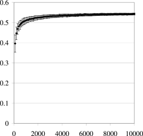
(a) $C(n)\ \big{/}\ (n^{2}\log{n})$

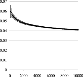
(b) $C(n)\ \big{/}\ (n^{2}\log^{2}{n})$

Figure 1: Experimental results of AHRSZ for the insertion of the edges of a complete DAG in a random order. The horizontal axes describe the number of vertices $n$. The vertical axes show the measured empirical insertion costs $C(n):=\sum_{i}{|\rangle K\langle|}\,\log{|\rangle K\langle|}$ relative to LABEL:sub@subfig:log $n^{2}\log{n}$ and LABEL:sub@subfig:log2 $n^{2}\log^{2}{n}$, respectively. The error bars specify the sample standard deviation.

The performance parameter taken for AHRSZ is $C(n):=\sum_{i}{|\rangle K\langle|}\,\log({{|\rangle K\langle|}})$. We know $\textup{{E}}\left[C(n)\right]={\cal O}(n^{2}\log^{3}{n})$ from Section 5 and know that the overall runtime is $\Omega(n^{2})$ since the algorithm has to inspect all the edges being inserted. In our experimental setting, we discovered that $C(n)/(n^{2}\log^{2}{n})$ is apparently a decreasing function and that $C(n)/(n^{2}\log{n})$ is an increasing function. This empirical evidence suggests that $C(n)$ is possibly between $\Omega(n^{2}\log{n})$ and ${\cal O}(n^{2}\log^{2}{n})$. Figure 1 shows our experimental results for AHRSZ.

We consider $C(n):=\sum_{i}({\|{\delta^{(i)}}\|}+{|{\delta^{(i)}}|}\log{{|{\delta^{(i)}}|}})$ as a performance parameter for PK and observe that $C(n)/n^{2}$ is decreasing while $C(n)/(n^{2}\log^{-1}{n})$ is increasing. This indicates that $C(n)=o(n^{2})$, which implies an actual runtime of $\Theta(n^{2})$ for PK on REIS since all $\Omega(n^{2})$ edges have to be inspected. Pearce and Kelly [19] showed empirically that PK outperforms AHRSZ on sparse DAGs. Our experiments extend this to dense DAGs.

Complementing Section 6, we also examined empirically the number of invalidating edges for AHRSZ. The same experimental set-up as above suggests a quasilinear growth of $\sum_{i=1}^{m}{\textsc{inval}(i)}$ between $\Omega(n\log{n})$ and ${\cal O}(n\log^{2}{n})$. Note that the observed empirical bound for AHRSZ is significantly lower than the general bound ${\cal O}(n^{\frac{3}{2}}\log^{\frac{1}{2}}{n})$ of Theorem 12 which holds for all algorithms.

8 Discussion

On random edge insertion sequences (REIS) leading to a complete DAG, we have shown an expected runtime of ${\cal O}(n^{2}\log^{2}{n})$ for PK and ${\cal O}(n^{2}\log^{3}{n})$ for AHRSZ and KB while the trivial lower bound is $\Omega(n^{2})$. Extending the average case analysis for the case where we only insert $m$ edges with $m\ll n^{2}$ still remains open. On the other hand, the only non-trivial lower bound for this problem is by Ramalingam and Reps [23], who have shown that an adversary can force any algorithm which maintains explicit labels to require $\Omega(n\log{n})$ time complexity for inserting $n-1$ edges. There is still a large gap between the lower bound of $\Omega(\max\{n\log{n},m\})$, the best average-case bound of ${\cal O}(n^{2}\log^{2}{n})$ and the worst-case bound of ${\cal O}(\min\{m^{1.5}+n^{2}\log{n},m^{1.5}\log{n},n^{2.75}\})$. Bridging this gap remains an open problem.

References

• Ajwani et al. [2006] D. Ajwani, T. Friedrich, and U. Meyer. An $O(n^{2.75})$ algorithm for online topological ordering. In Proceedings of the Scandinavian Workshop on Algorithm Theory (SWAT ’06), Vol. 4059 of Lecture Notes in Computer Science, pp. 53–64, 2006.
• Alpern et al. [1990] B. Alpern, R. Hoover, B. K. Rosen, P. F. Sweeney, and F. K. Zadeck. Incremental evaluation of computational circuits. In Proceedings of the ACM-SIAM Symposium on Discrete Algorithms (SODA ’90), pp. 32–42, 1990.
• Ausiello et al. [1991] G. Ausiello, G. F. Italiano, A. Marchetti-Spaccamela, and U. Nanni. Incremental algorithms for minimal length paths. J. Algorithms, 12:615–638, 1991.
• Barak and Erdős [1984] A. B. Barak and P. Erdős. On the maximal number of strongly independent vertices in a random acyclic directed graph. SIAM Journal on Algebraic and Discrete Methods, 5:508–514, 1984.
• Bollobás [1981] B. Bollobás. Degree sequences of random graphs. Discrete Math., 33:1–19, 1981.
• Bollobás [2001] B. Bollobás. Random Graphs. Cambridge Univ. Press, 2001.
• Cicerone et al. [1998] S. Cicerone, D. Frigioni, U. Nanni, and F. Pugliese. A uniform approach to semi-dynamic problems on digraphs. Theor. Comput. Sci., 203:69–90, 1998.
• Cormen et al. [1989] T. Cormen, C. Leiserson, and R. Rivest. Introduction to Algorithms. The MIT Press, Cambridge, MA, 1989.
• Dietz and Sleator [1987] P. F. Dietz and D. D. Sleator. Two algorithms for maintaining order in a list. In Proceedings of the ACM Symposium on Theory of Computing (STOC ’87), pp. 365–372, 1987.
• Eppstein et al. [1999] D. Eppstein, Z. Galil, and G. F. Italiano. Dynamic graph algorithms. In M. J. Atallah, editor, Algorithms and Theory of Computation Handbook, chapter 8. CRC Press, 1999.
• Erdős and Rényi [1959] P. Erdős and A. Rényi. On random graphs. Publ Math Debrecen, 6:290–297, 1959.
• Erdős and Rényi [1960] P. Erdős and A. Rényi. On the evolution of random graphs. Magyar Tud. Akad. Mat. Kutato Int. Kozl., 5:17–61, 1960.
• Frigioni et al. [1998] D. Frigioni, A. Marchetti-Spaccamela, and U. Nanni. Fully dynamic shortest paths and negative cycles detection on digraphs with arbitrary arc weights. In Proceedings of the European Symposium on Algorithms (ESA ’98), Vol. 1461 of Lecture Notes in Computer Science, pp. 320–331, 1998.