On the distribution of the free path length of
the linear flow in a honeycomb

Abstract.

Let $\ell\geqslant 2$ be an integer. For each $\varepsilon\in(0,\frac{1}{2})$ remove from $\mathbb{R}^{2}$ the union of discs of radius $\varepsilon$ centered at the integer lattice points $(m,n)$, with $m\nequiv n\pmod{\ell}$. Consider a point-like particle moving linearly at unit speed, with velocity $\omega$, along a trajectory starting at the origin, and its free path length $\tau_{\ell,\varepsilon}(\omega)\in[0,\infty]$. We prove the weak convergence of the probability measures associated with the random variables $\varepsilon\tau_{\ell,\varepsilon}$ as $\varepsilon\rightarrow 0^{+}$ and explicitly compute the limiting distribution. For $\ell=3$ this leads to an asymptotic formula for the length of the trajectory of a billiard in a regular hexagon, starting at the center, with circular pockets of radius $\varepsilon\rightarrow 0^{+}$ removed from the corners. For $\ell=2$ this corresponds to the trajectory of a billiard in a unit square with circular pockets removed from the corners and trajectory starting at the center of the square. The limiting probability measures on $[0,\infty)$ have a tail at infinity, which contrasts with the case of a square with pockets and trajectory starting from one of the corners, where the limiting probability measure has compact support.

1. Introduction

Recent progress led to a better understanding of the statistics of the free path length of the periodic Lorentz gas in the small scatterer limit [2, 3, 5, 6, 7, 8, 9, 10]. The aim of this paper is to study situations where periodicity conditions are altered by imposing certain congruence conditions on the integer lattice points where scatterers are placed. The case of the honeycomb lattice arises as a particular example in this context. Here we only consider the situation where motion originates at the origin, extending the results from [2] and [3]. The case where the initial position is randomly chosen is more intricate and will not be treated here.

Let $\ell\geqslant 2$ be an integer. Consider the set $\mathbb{Z}^{2}_{(\ell)}$ of pairs of integers $(m,n)$ with $m\nequiv n\pmod{\ell}$. For every $\varepsilon>0$ consider the “fat lattice points” (scatterers) given by small discs of radius $\varepsilon$ centered at all points of $\mathbb{Z}^{2}_{(\ell)}$ and the region

$$Z_{\ell,\varepsilon}=\{x\in\mathbb{R}^{2}:\operatorname{dist}(x,\mathbb{Z}^{2}_{(\ell)})\geqslant\varepsilon\}$$

obtained by removing all scatterers. In $\mathbb{R}^{2}$ consider a point-like particle moving at constant unit speed along a linear trajectory originating at $(0,0)$. The free path length (first exit time) is defined as

$$\tau_{\ell,\varepsilon}(\omega)=\inf\{\tau>0:\tau\vec{\omega}\in\partial Z_{\ell,\varepsilon}\},$$

the distance traveled to reach the first scatterer along the direction $\vec{\omega}=e^{i\omega}\in{\mathbb{T}}$, $\omega\in[0,2\pi)$, and as $+\infty$ when the particle escapes to infinity without reaching any scatterer. The Lebesgue measure of a measurable set $A\subseteq\mathbb{R}$ is denoted by $|A|$. This paper is concerned with the study, in the small scatterer limit ($\varepsilon\rightarrow 0^{+}$), of the asymptotic behavior of the repartition function of $\varepsilon\tau_{\ell,\varepsilon}$ defined by

$${\mathbb{P}}_{\ell,\varepsilon}(\lambda)=\frac{1}{2\pi}\bigg{|}\bigg{\{}\omega\in[0,2\pi):\tau_{\ell,\varepsilon}(\omega)>\frac{\lambda}{\varepsilon}\bigg{\}}\bigg{|}.$$

To accomplish this we first consider the situation where scatterers are obtained by translating the vertical segment $V_{\varepsilon}=\{0\}\times[-\varepsilon,\varepsilon]$ by $(m,n)\in\mathbb{Z}^{2}_{(\ell)}$ and estimate, for any interval $I\subseteq[0,1]$ of length $|I|\asymp\varepsilon^{c}$ with fixed $c\in(0,1)$, the repartition

$${\mathbb{G}}_{\ell,I,\varepsilon}(\lambda)=\left|\left\{\omega\in\arctan I:q_{\ell,\varepsilon}(\omega)>\frac{\lambda}{\varepsilon}\right\}\right|,\qquad\varepsilon\rightarrow 0^{+},$$

of the horizontal free path length

$$q_{\ell,\varepsilon}(\omega)=\inf\left\{q:(q,q\tan\omega)\in\mathbb{Z}^{2}_{(\ell)}+V_{\varepsilon}\right\},\qquad\omega\in\bigg{[}0,\frac{\pi}{4}\bigg{]}.$$

In this paper $\varphi$ will denote Euler’s totient function. The dilogarithm is defined by

$$\operatorname{Li}_{2}(x)=\sum\limits_{n=1}^{\infty}\frac{x^{n}}{n^{2}}=-\int_{0}^{x}\frac{\ln(1-t)}{t}\,dt,\qquad x\in[0,1].$$

Clearly $\operatorname{Li}_{2}(1)=\zeta(2)=\frac{\pi^{2}}{6}$.

The main result of this paper shows that the limit of $\mathbb{P}_{\ell,\varepsilon}$ exists as $\varepsilon\rightarrow 0^{+}$ and this limit is explicitly computed.

Theorem 1.

(i) For every $0<c_{1}<1$ and $\delta>0$, as $\varepsilon\rightarrow 0^{+}$,

$${\mathbb{G}}_{\ell,I,\varepsilon}(\lambda)=c_{I}G_{\ell}(\lambda)+O_{\delta,\lambda,\ell}\left(\varepsilon^{-\delta+\theta(c,c_{1})}\right),\qquad\lambda>0,$$ (1.1)

where

$$c_{I}=\int_{I}\frac{du}{1+u^{2}},\qquad\theta(c,c_{1})=\min\bigg{\{}c+c_{1},\frac{1}{2}-2c_{1}\bigg{\}},$$

and the limiting repartition function $G_{\ell}$ is given by

$$G_{\ell}(\lambda)=\begin{cases}\vspace{.1cm}1-\left(\frac{1}{\zeta(2)}+A(\ell)\right)\lambda&\mbox{\rm if $\ \lambda\in\big{(}0,\frac{1}{2}\big{]},$}\\ \vspace{.1cm}1-\frac{\lambda}{\zeta(2)}+A(\ell)H_{2}(\lambda)&\mbox{\rm if $\ \lambda\in\big{[}\frac{1}{2},1\big{]},$}\\ \frac{2C(\ell)}{\ell}H_{3}(\lambda)&\mbox{\rm if $\ \lambda\in[1,\infty),$}\end{cases}$$

with

$$\begin{split}C(\ell)&=\frac{\varphi(\ell)}{\zeta(2)\ell}\prod\limits_{\begin{subarray}{c}p\mid\ell\\ p\operatorname{prime}\end{subarray}}\left(1-\frac{1}{p^{2}}\right)^{-1}=\frac{\varphi(\ell)}{\ell}\prod\limits_{\begin{subarray}{c}p\nmid\ell\\ p\operatorname{prime}\end{subarray}}\left(1-\frac{1}{p^{2}}\right),\quad A(\ell)=\frac{1}{\zeta(2)}-\frac{2C(\ell)}{\ell},\\ H_{2}(\lambda)&=3\lambda-2+\zeta(2)-(\ln\lambda)^{2}+2(1-\lambda)\ln\left(\frac{1}{\lambda}-1\right)-2\operatorname{Li}_{2}(\lambda),\\ H_{3}(\lambda)&=\operatorname{Li}_{2}\left(\frac{1}{\lambda}\right)-(\lambda-1)\ln\left(1-\frac{1}{\lambda}\right)-1.\end{split}$$ (1.2)

(ii) For every $\delta>0$, as $\varepsilon\rightarrow 0^{+}$,

$${\mathbb{P}}_{\ell,\varepsilon}(\lambda)=G_{\ell}(\lambda)+O_{\delta,\lambda,\ell}\left(\varepsilon^{\frac{1}{8}+\delta}\right),\qquad\lambda>0.$$

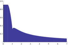
Figure 1. The repartition function $G_{3}$ and the density function $g_{3}$

The continuity of $G_{\ell}$ at $\lambda=\frac{1}{2}$ is equivalent with the well known dilogarithm identity

$$\sum_{n=1}^{\infty}\frac{1}{2^{n}n^{2}}=\operatorname{Li}_{2}\left(\frac{1}{2}\right)=\int_{0}^{1/2}\frac{1}{u}\ \ln\frac{1}{1-u}\ du=\frac{\zeta(2)-(\ln 2)^{2}}{2}.$$

Since $\frac{C(\ell)}{\ell}\rightarrow 0$ and $A(\ell)\rightarrow\frac{1}{\zeta(2)}$ as $\ell\rightarrow\infty$, the compactly supported limiting repartition $H(\lambda)$ from [2, Theorem 1.1] is being recovered as $\lim_{\ell\rightarrow\infty}G_{\ell}(\lambda)$.

Figure 2. The free path in a hexagonal billiard and in a honeycomb

Our original motivation for considering this problem comes from the study of the exit time of the linear motion with specular cushion collisions on a hexagonal (open) billiard table with (small) circular open pockets of radius $\varepsilon$ removed from its corners (see Figure 2). The starting remark here is that, after unfolding the hexagon to a honeycomb in $\mathbb{R}^{2}$, one can deform the later to $\mathbb{Z}^{2}_{(3)}$. This process converts the problem on the hexagonal billiard with pockets into one concerning the free path length of a Lorentz gas in $\mathbb{R}^{2}$ with small identical ellipses centered at the points from $\mathbb{Z}^{2}_{(3)}$ as scatterers (see Figure 8).

Let $\tau^{\,\operatorname{hex}}_{\varepsilon}(\omega)$ denote the free path length in the hexagonal billiard with discs of radius $\varepsilon$ removed from the corners and motion starting at the center, and let

$${\mathbb{P}}^{\,\operatorname{hex}}_{\varepsilon}(\lambda)=\frac{1}{2\pi}\bigg{|}\bigg{\{}\omega\in[0,2\pi]:\tau^{\,\operatorname{hex}}_{\varepsilon}(\omega)>\frac{\lambda}{\varepsilon}\bigg{\}}\bigg{|}$$

denote the repartition function of $\varepsilon\tau^{\,\operatorname{hex}}_{\varepsilon}$. We prove

Theorem 2.

For every $\delta>0$, as $\varepsilon\rightarrow 0^{+}$,

$${\mathbb{P}}^{\,\operatorname{hex}}_{\varepsilon}(\lambda)=G_{3}\left(\frac{2\lambda}{\sqrt{3}}\right)+O_{\delta}\left(\varepsilon^{\frac{1}{8}-\delta}\right),\qquad\lambda>0.$$

Scaling $\varepsilon$ to $\varepsilon\sqrt{2}$ one can apply Theorem 1 (ii) with $\ell=2$ to estimate the repartition function ${\mathbb{P}}^{\square}_{\varepsilon}(\lambda)=\frac{1}{2\pi}|\{\omega\in[0,2\pi]:\tau_{\varepsilon}^{\square}(\omega)>\frac{\lambda}{\varepsilon}\}|$ of the free path length $\tau_{\varepsilon}^{\square}(\omega)$ of a billiard in the unit square with pockets of radius $\varepsilon$ at the corners and trajectory starting at the center (see Figure 3), getting

Theorem 3.

For every $\delta>0$, as $\varepsilon\rightarrow 0^{+}$,

$${\mathbb{P}}^{\square}_{\varepsilon}(\lambda)=G_{2}\left(\frac{\lambda}{\sqrt{2}}\right)+O_{\delta}\Big{(}\varepsilon^{\frac{1}{8}-\delta}\Big{)},\qquad\lambda>0.$$

Figure 3. The free path in a square billiard with trajectory starting at the center

Theorem 3 should be compared with the situation where the initial position is at one of the four vertices, and where the limiting distribution has compact support [2, 3]. It is not clear whether these methods would directly extend to other concrete initial positions, such as $(\frac{1}{n},0)$, $n\in\mathbb{N}$. However, it looks likely that further refinements could lead to “space-phase average” results similar to those from [5]. The main difficulty seems to arise from the increasing complexity and number of cases that need to be analyzed in detail, leading to integrals in the main terms of the asymptotic formula which are manifestly more intricate than in the case of the square.

2. The contribution of consecutive Farey fractions $\gamma<\gamma^{\prime}$ with $\gamma,\gamma^{\prime}\in\mathcal{F}_{Q}\setminus\mathcal{F}^{(\ell)}$

The integer part of a real number $x$ is denoted by $[x]$. Let $\varepsilon>0$ and $Q=\big{[}\frac{1}{\varepsilon}\big{]}$. Denote by $\mathcal{F}_{Q}$ the set of Farey fractions $\gamma=\frac{a}{q}$ in lowest terms with $0<a\leqslant q\leqslant Q$. For any interval $I\subseteq[0,1]$, set $\mathcal{F}_{I,Q}=I\cap\mathcal{F}_{Q}$. Denote by $\mathcal{F}_{Q}^{(\ell)}$ the set of Farey fractions $\gamma=\frac{a}{q}\in\mathcal{F}_{Q}$ with $\ell\mid(q-a)$, and set $\mathcal{F}^{(\ell)}_{I,Q}=I\cap\mathcal{F}_{Q}^{(\ell)}$. Set also $\mathcal{F}^{(\ell)}=\cup_{Q=1}^{\infty}\mathcal{F}_{Q}^{(\ell)}$. It is well known that if $\gamma=\frac{a}{q}<\gamma^{\prime}=\frac{a^{\prime}}{q^{\prime}}$ are consecutive elements in $\mathcal{F}_{Q}$ if and only if

$$a^{\prime}q-aq^{\prime}=1\quad\mbox{\rm and}\quad q+q^{\prime}>Q\geqslant\max\{q,q^{\prime}\}.$$

In particular we have

$$\varepsilon(q+q^{\prime})\geqslant\varepsilon(Q+1)>1\geqslant\max\{\varepsilon q,\varepsilon q^{\prime}\}.$$ (2.1)

For convenience consider

$$\tilde{\mathbb{G}}_{\ell,I,\varepsilon}(\lambda):=\big{|}\{\omega\in\arctan I:q_{\ell,\varepsilon}(\omega)>\lambda Q\}\big{|}={\mathbb{G}}_{\ell,I,\varepsilon}\bigg{(}\lambda\varepsilon\bigg{[}\frac{1}{\varepsilon}\bigg{]}\Bigg{)},\quad\lambda>0.$$

For any interval $I\subseteq[0,1]$ with $|I|\asymp Q^{-c}$, $0<c<1$, we will prove a formula of type

$$\tilde{\mathbb{G}}_{\ell,I,\varepsilon}(\lambda)=c_{I}G_{\ell}(\lambda)+O_{\delta}\left(\varepsilon^{-\delta+\theta(c,c_{1})}\right),$$

which will immediately imply (1.1), because $\varepsilon\big{[}\frac{1}{\varepsilon}\big{]}=1+O(\varepsilon)$ and for any compact set $K\subseteq\mathbb{R}_{+}$ there is $C_{K}>0$ such that

$$|G_{\ell}(x^{\prime})-G_{\ell}(x^{\prime\prime})|\leqslant C_{K}|x^{\prime}-x^{\prime\prime}|,\qquad x^{\prime},x^{\prime\prime}\in K.$$ (2.2)

Given $\gamma<\gamma^{\prime}$ consecutive elements in $\mathcal{F}_{Q}$, denote $t_{0}=\gamma^{\prime}-\frac{\varepsilon}{q^{\prime}}=\frac{a^{\prime}-\varepsilon}{q^{\prime}}$, $u_{0}=\gamma+\frac{\varepsilon}{q}=\frac{a+\varepsilon}{q}$. Employing (2.1) and

$$t_{0}-\gamma=\frac{1-\varepsilon q}{qq^{\prime}},\qquad u_{0}-t_{0}=\frac{\varepsilon(q+q^{\prime})-1}{qq^{\prime}},\qquad\gamma^{\prime}-u_{0}=\frac{1-\varepsilon q^{\prime}}{qq^{\prime}},$$ (2.3)

we find $\gamma\leqslant t_{0}<u_{0}\leqslant\gamma^{\prime}$. In particular if $\gamma<\gamma^{\prime}<\gamma^{\prime\prime}$ are consecutive elements in $\mathcal{F}_{Q}$, then $\gamma+\frac{\varepsilon}{q}\leqslant\gamma^{\prime}<\gamma^{\prime\prime}-\frac{\varepsilon}{q^{\prime\prime}}$. Therefore the intervals $[\gamma-\frac{\varepsilon}{q},\gamma+\frac{\varepsilon}{q}]$, $\gamma=\frac{a}{q}\in\mathcal{F}_{Q}$, cover the interval $[0,1]$ in such a way that every element in $[0,1]$ belongs to at most two of these intervals. As a result any trajectory with slope $\tan\omega\in(\gamma,\gamma^{\prime})$ will intersect, as in the case of the square lattice [2, 3], one of the scatterers $(q,a)+V_{\varepsilon}$ or $(q^{\prime},a^{\prime})+V_{\varepsilon}$.

Since $a^{\prime}q-aq^{\prime}=1$, only two situations can occur here: $\gamma\notin\mathcal{F}^{(\ell)}$ and $\gamma^{\prime}\notin\mathcal{F}^{(\ell)}$, respectively $\gamma\in\mathcal{F}^{(\ell)}$ or $\gamma^{\prime}\in\mathcal{F}^{(\ell)}$. The later will be discussed in Section 3. In the remainder of this section we assume that $\gamma\notin\mathcal{F}^{(\ell)}$ and $\gamma^{\prime}\notin\mathcal{F}^{(\ell)}$, situation where the horizontal free path is given (see Figure 4) by

$$q_{\ell,\varepsilon}(\omega)=\begin{cases}q&\mbox{\rm if $\ \gamma<\tan\omega<t_{0},$}\\ \min\{q,q^{\prime}\}&\mbox{\rm if $\ t_{0}<\tan\omega<u_{0},$}\\ q^{\prime}&\mbox{\rm if $\ u_{0}<\tan\omega<\gamma^{\prime}.$}\end{cases}$$

Figure 4. The horizontal free path when $\gamma,\gamma^{\prime}\in\mathcal{F}_{I,Q}\setminus\mathcal{F}^{(\ell)}$

In this way the contribution of the interval $[\gamma,\gamma^{\prime}]$ to $\tilde{\mathbb{G}}_{\ell,I,\varepsilon}(\lambda)$ is given by

$$\begin{cases}0&\mbox{\rm if $\ \max\{q,q^{\prime}\}\leqslant\lambda Q,$}\\ \arctan\gamma^{\prime}-\arctan\gamma&\mbox{\rm if $\ \min\{q,q^{\prime}\}>\lambda Q,$}\\ \arctan\gamma^{\prime}-\arctan u_{0}&\mbox{\rm if $\ q\leqslant\lambda Q<q^{\prime},$}\\ \arctan t_{0}-\arctan\gamma&\mbox{\rm if $\ q^{\prime}\leqslant\lambda Q<q.$}\end{cases}$$

This contribution is zero whenever $\lambda\geqslant 1$, so we next assume $0<\lambda<1$.

Using (2.3), the estimates

$$\arctan(x+h)-\arctan x=\frac{h}{1+x^{2}}+O(h^{2}),\qquad\frac{1}{1+\gamma^{2}}-\frac{1}{1+\gamma^{\prime 2}}\leqslant 2(\gamma^{\prime}-\gamma)=\frac{2}{qq^{\prime}},$$ (2.4)

and the inequality

$$\sum_{\gamma\in\mathcal{F}_{Q}}\frac{1}{q^{2}q^{\prime 2}}\leqslant\sum_{\gamma\in\mathcal{F}_{Q}}\frac{1}{Qqq^{\prime}}=\frac{1}{Q},$$

we infer that the contribution to $\tilde{\mathbb{G}}_{\ell,I,\varepsilon}(\lambda)$ of all intervals $[\gamma,\gamma^{\prime}]\subseteq I$ with $\gamma<\gamma^{\prime}$ consecutive elements in $\mathcal{F}_{Q}$ and $\gamma,\gamma^{\prime}\notin\mathcal{F}^{(\ell)}$ is given by

$${\mathbb{G}}^{(1)}_{\ell,I,\varepsilon}(\lambda)=A_{I,Q}(\lambda)+B_{I,Q}(\lambda)+C_{I,Q}(\lambda)+O(\varepsilon),$$

with

$$A_{I,Q}(\lambda)=\sum\limits_{\begin{subarray}{c}\gamma,\gamma^{\prime}\in\mathcal{F}_{I,Q}\setminus\mathcal{F}^{(\ell)}\\ \min\{q,q^{\prime}\}>\lambda Q\end{subarray}}\frac{1}{qq^{\prime}}\cdot\frac{1}{1+\gamma^{2}},$$ (2.5)

$$B_{I,Q}(\lambda)=\sum\limits_{\begin{subarray}{c}\gamma,\gamma^{\prime}\in\mathcal{F}_{I,Q}\setminus\mathcal{F}^{(\ell)}\\ q\leqslant\lambda Q<q^{\prime}\end{subarray}}\frac{1-\varepsilon q^{\prime}}{qq^{\prime}}\cdot\frac{1}{1+\gamma^{\,\prime\,2}},\qquad C_{I,Q}(\lambda)=\sum\limits_{\begin{subarray}{c}\gamma,\gamma^{\prime}\in\mathcal{F}_{I,Q}\setminus\mathcal{F}^{(\ell)}\\ q^{\prime}\leqslant\lambda Q<q\end{subarray}}\frac{1-\varepsilon q}{qq^{\prime}}\cdot\frac{1}{1+\gamma^{2}}.$$ (2.6)

Since there are no consecutive elements in $\mathcal{F}_{Q}$ which belong both to $\mathcal{F}^{(\ell)}$ we have

$$A_{I,Q}(\lambda)=A^{+}_{I,Q}(\lambda)-A_{I,Q}^{-,1}(\lambda)-A_{I,Q}^{-,2}(\lambda),$$ (2.7)

with

$$\begin{split}A_{I,Q}^{+}(\lambda)&=\sum_{\begin{subarray}{c}\gamma,\gamma^{\prime}\in\mathcal{F}_{I,Q}\\ \min\{q,q^{\prime}\}>\lambda Q\end{subarray}}\frac{1}{qq^{\prime}}\cdot\frac{1}{1+\gamma^{2}},\\ A_{I,Q}^{-,1}(\lambda)&=\sum_{\begin{subarray}{c}\gamma\in\mathcal{F}_{I,Q}^{(\ell)},\,\gamma^{\prime}\in\mathcal{F}_{I,Q}\\ \min\{q,q^{\prime}\}>\lambda Q\end{subarray}}\frac{1}{qq^{\prime}}\cdot\frac{1}{1+\gamma^{2}},\qquad A_{I,Q}^{-,2}(\lambda)=\sum_{\begin{subarray}{c}\gamma\in\mathcal{F}_{I,Q},\,\gamma^{\prime}\in\mathcal{F}_{I,Q}^{(\ell)}\\ \min\{q,q^{\prime}\}>\lambda Q\end{subarray}}\frac{1}{qq^{\prime}}\cdot\frac{1}{1+\gamma^{2}},\end{split}$$

and respectively

$$B_{I,Q}(\lambda)=B_{I,Q}^{+}(\lambda)-B_{I,Q}^{-,1}(\lambda)-B_{I,Q}^{-,2}(\lambda),\qquad C_{I,Q}(\lambda)=C_{I,Q}^{+}(\lambda)-C_{I,Q}^{-,1}(\lambda)-C_{I,Q}^{-,2}(\lambda),$$ (2.8)

with

$$\begin{split}&B_{I,Q}^{+}(\lambda)=\sum_{\begin{subarray}{c}\gamma,\gamma^{\prime}\in\mathcal{F}_{I,Q}\\ q\leqslant\lambda Q<q^{\prime}\end{subarray}}\frac{1-\varepsilon q^{\prime}}{qq^{\prime}}\cdot\frac{1}{1+\gamma^{\,\prime\,2}},\qquad\quad\ \ C_{I,Q}^{+}(\lambda)=\sum\limits_{\begin{subarray}{c}\gamma,\gamma^{\prime}\in\mathcal{F}_{I,Q}\\ q^{\prime}\leqslant\lambda Q<q\end{subarray}}\frac{1-\varepsilon q}{qq^{\prime}}\cdot\frac{1}{1+\gamma^{2}},\\ &B_{I,Q}^{-,1}(\lambda)=\sum_{\begin{subarray}{c}\gamma\in\mathcal{F}_{I,Q}^{(\ell)},\,\gamma^{\prime}\in\mathcal{F}_{I,Q}\\ q\leqslant\lambda Q<q^{\prime}\end{subarray}}\frac{1-\varepsilon q^{\prime}}{qq^{\prime}}\cdot\frac{1}{1+\gamma^{\,\prime\,2}},\qquad C_{I,Q}^{-,1}(\lambda)=\sum\limits_{\begin{subarray}{c}\gamma\in\mathcal{F}_{I,Q}^{(\ell)},\,\gamma^{\prime}\in\mathcal{F}_{I,Q}\\ q^{\prime}\leqslant\lambda Q<q\end{subarray}}\frac{1-\varepsilon q}{qq^{\prime}}\cdot\frac{1}{1+\gamma^{2}},\\ &B_{I,Q}^{-,2}(\lambda)=\sum_{\begin{subarray}{c}\gamma\in\mathcal{F}_{I,Q},\,\gamma^{\prime}\in\mathcal{F}_{I,Q}^{(\ell)}\\ q\leqslant\lambda Q<q^{\prime}\end{subarray}}\frac{1-\varepsilon q^{\prime}}{qq^{\prime}}\cdot\frac{1}{1+\gamma^{\,\prime\,2}},\qquad C_{I,Q}^{-,2}(\lambda)=\sum\limits_{\begin{subarray}{c}\gamma,\gamma^{\prime}\in\mathcal{F}_{I,Q}\\ q^{\prime}\leqslant\lambda Q<q\end{subarray}}\frac{1-\varepsilon q}{qq^{\prime}}\cdot\frac{1}{1+\gamma^{2}}.\end{split}$$

Lemma 1.

For any function $V\in C^{1}[0,N]$ with total variation $T_{0}^{N}V$ and $C(\ell)$ as in (1.2),

$$\sum\limits_{\begin{subarray}{c}1\leqslant k\leqslant N\\ \gcd(\ell,k)=1\end{subarray}}\frac{\varphi(k)}{k}\,V(k)=C(\ell)\int_{0}^{N}V+O_{\ell}\Big{(}(\|V\|_{\infty}+T_{0}^{N}V)\ln N\Big{)}.$$

Proof.

The left-hand side $L_{\ell,N}$ can be expressed as

$$\sum\limits_{\begin{subarray}{c}1\leqslant k\leqslant N\\ \gcd(\ell,k)=1\end{subarray}}\sum\limits_{d\mid k}\frac{\mu(d)}{d}\,V(k).$$

Writing $k=dk^{\prime}$ with $1\leqslant k^{\prime}\leqslant[\frac{N}{d}]$ and $\gcd(\ell,d)=\gcd(\ell,k^{\prime})=1$, denoting $V_{n}(x)=V(nx)$, $\sigma_{0}(\ell):=\#\{d\geqslant 1:d\mid\ell\}$, and using Möbius summation (as in [1, Lemma 2.2]) we have

$$\begin{split}L_{\ell,N}&=\sum\limits_{\begin{subarray}{c}1\leqslant d\leqslant N\\ \gcd(\ell,d)=1\end{subarray}}\frac{\mu(d)}{d}\sum\limits_{\begin{subarray}{c}1\leqslant k^{\prime}\leqslant[N/d]\\ \gcd(\ell,k^{\prime})=1\end{subarray}}V_{d}(k^{\prime})\\ &=\sum\limits_{\begin{subarray}{c}1\leqslant d\leqslant N\\ \gcd(\ell,d)=1\end{subarray}}\frac{\mu(d)}{d}\left(\frac{\varphi(\ell)}{\ell}\int_{0}^{[N/d]}V_{d}+O\bigg{(}\Big{(}\|V_{d}\|_{\infty}+T_{0}^{[N/d]}V_{d}\Big{)}\sigma_{0}(\ell)\right)\\ &=\frac{\varphi(\ell)}{\ell}\sum\limits_{\begin{subarray}{c}1\leqslant d\leqslant N\\ \gcd(\ell,d)=1\end{subarray}}\frac{\mu(d)}{d}\cdot\frac{1}{d}\left(\int_{0}^{N}V+O\big{(}d\|V\|_{\infty}\big{)}\right)+O_{\ell}\Bigg{(}\big{(}\|V\|_{\infty}+T_{0}^{N}V\big{)}\sum_{d=1}^{N}\frac{1}{d}\Bigg{)}\\ &=\frac{\varphi(\ell)}{\ell}\sum\limits_{\begin{subarray}{c}1\leqslant d\leqslant N\\ \gcd(\ell,d)=1\end{subarray}}\frac{\mu(d)}{d^{2}}\int_{0}^{N}V+O\big{(}\|V\|_{\infty}\ln N\big{)}+O_{\ell}\Big{(}\big{(}\|V\|_{\infty}+T_{0}^{N}V\big{)}\ln N\Big{)}\\ &=\frac{\varphi(\ell)}{\ell}\Bigg{(}\sum\limits_{\begin{subarray}{c}d\geqslant 1\\ \gcd(\ell,d)=1\end{subarray}}\frac{\mu(d)}{d^{2}}+O\bigg{(}\sum_{d>N}\frac{1}{d^{2}}\bigg{)}\Bigg{)}\int_{0}^{N}V+O_{\ell}\Big{(}\big{(}\|V\|_{\infty}+T_{0}^{N}V\big{)}\ln N\Big{)}\\ &=C(\ell)\int_{0}^{N}V+O_{\ell}\Big{(}(\|V\|_{\infty}+T_{0}^{N}V)\ln N\Big{)},\end{split}$$

with

$$C(\ell)=\frac{\varphi(\ell)}{\ell}\sum\limits_{\begin{subarray}{c}d\geqslant 1\\ \gcd(\ell,d)=1\end{subarray}}\frac{\mu(d)}{d^{2}}=\frac{\varphi(\ell)}{\ell}\prod\limits_{\begin{subarray}{c}p\nmid\ell\\ p\operatorname{prime}\end{subarray}}\left(1-\frac{1}{p^{2}}\right)=\frac{\varphi(\ell)}{\zeta(2)\ell}\prod\limits_{\begin{subarray}{c}p\mid\ell\\ p\operatorname{prime}\end{subarray}}\left(1-\frac{1}{p^{2}}\right)^{-1},$$

which gives the desired estimate. ∎

Lemma 2.

For any function $V\in C^{1}[0,N]$ and any $\delta>0$,

$$\sum_{n=1}^{N}\frac{\varphi(\ell n)}{n}\ V(n)=\ell C(\ell)\int_{0}^{N}V+O_{\ell,\delta}\left((\|V\|_{\infty}+T_{0}^{N}V)N^{\delta}\right).$$

Proof.

Let $\ell=p_{1}^{\alpha_{1}}\cdots p_{r}^{\alpha_{r}}$ with $p_{1},\ldots,p_{r}$ distinct primes and $\alpha_{1},\ldots,\alpha_{r}\in\mathbb{N}$ (so $r=\omega(\ell)$, the number of prime divisors of $\ell$). Writing $n=p_{1}^{k_{1}}\cdots p_{r}^{k_{r}}m$ with $k_{i}\geqslant 0$ and $\gcd(\ell,m)=1$, we obtain

$$\sum\limits_{1\leqslant n\leqslant N}\frac{\varphi(\ell n)}{n}\ V(n)=\sum\limits_{\begin{subarray}{c}k_{1},\ldots,k_{r}\geqslant 0\\ p_{1}^{k_{1}}\cdots p_{r}^{k_{r}}\leqslant N\end{subarray}}\prod_{1\leqslant i\leqslant r}\frac{\varphi(p_{i}^{k_{i}+\alpha_{i}})}{p_{i}^{k_{i}}}\sum\limits_{\begin{subarray}{c}1\leqslant m\leqslant N/(p_{1}^{k_{1}}\cdots p_{r}^{k_{r}})\\ \gcd(\ell,m)=1\end{subarray}}\frac{\varphi(m)}{m}\ V_{p_{1}^{k_{1}}\cdots p_{r}^{k_{r}}}(m).$$ (2.9)

According to Lemma 1 the inner sum above can be expressed as

$$\begin{split}C(\ell)\int_{0}^{N/(p_{1}^{k_{1}}\cdots p_{r}^{k_{r}})}&V(p_{1}^{k_{1}}\cdots p_{r}^{k_{r}}x)\ dx+O_{\ell}\left((\|V\|_{\infty}+T_{0}^{N}V)\ln N\right)\\ &=\frac{C(\ell)}{p_{1}^{k_{1}}\cdots p_{r}^{k_{r}}}\int_{0}^{N}V+O_{\ell}\left((\|V\|_{\infty}+T_{0}^{N}V)\ln N\right).\end{split}$$

Inserting this into (2.9) and using the fact that the number of terms in the first sum in (2.9) is $\ll(\ln N)^{\omega(\ell)}$ and $\varphi(p_{i}^{k_{i}+\alpha_{i}})=p_{i}^{k_{i}+\alpha_{i}}(1-p_{i}^{-1})$ we infer that the expression in (2.9) is given by

$$\ell C(\ell)\prod\limits_{\begin{subarray}{c}p\mid\ell\\ p\operatorname{prime}\end{subarray}}\left(1-\frac{1}{p}\right)\sum\limits_{\begin{subarray}{c}k_{1},\ldots,k_{r}\geqslant 0\\ p_{1}^{k_{1}}\cdots p_{r}^{k_{r}}\leqslant N\end{subarray}}\frac{1}{p_{1}^{k_{1}}\cdots p_{r}^{k_{r}}}\int_{0}^{N}V+O_{\ell}\left((\|V\|_{\infty}+T_{0}^{N}V)(\ln N)^{1+\omega(\ell)}\right).$$ (2.10)

The statement now follows from (2.10), using

$$\sum_{k_{1},\ldots,k_{r}\geqslant 0}\frac{1}{p_{1}^{k_{1}}\cdots p_{r}^{k_{r}}}=\prod\limits_{\begin{subarray}{c}p\mid\ell\\ p\operatorname{prime}\end{subarray}}\left(1-\frac{1}{p}\right)^{-1}$$

and the bound

$$\sum_{\begin{subarray}{c}k_{1},\ldots,k_{r}\geqslant 0\\ p_{1}^{k_{1}}\cdots p_{r}^{k_{r}}>N\end{subarray}}\frac{1}{p_{1}^{k_{1}}\cdots p_{r}^{k_{r}}}\ll_{p_{1},\ldots,p_{r}}\frac{(\ln N)^{r-1}}{N}.$$

∎

The following estimate [4, Proposition A4] will be employed several times.

Lemma 3.

Assume that $q\geqslant 1$ and $h$ are two given integers, $\mathcal{I}$ and $\mathcal{J}$ are intervals of length less than $q$, and $f:\mathcal{I}\times\mathcal{J}\rightarrow\mathbb{R}$ is a $C^{1}$ function. Then for any integer $T>1$ and any $\delta>0$

$$\sum\limits_{\begin{subarray}{c}a\in\mathcal{I},b\in\mathcal{J}\\ ab=h\pmod{q}\\ \gcd(b,q)=1\end{subarray}}f(a,b)=\frac{\varphi(q)}{q^{2}}\iint_{\mathcal{I}\times\mathcal{J}}f(x,y)\,dxdy+\mathcal{E},$$

with

$$\mathcal{E}\ll_{\delta}T^{2}\|f\|_{\infty}q^{\frac{1}{2}+\delta}\gcd(h,q)^{\frac{1}{2}}+T\|\nabla f\|_{\infty}q^{\frac{3}{2}+\delta}\gcd(h,q)^{\frac{1}{2}}+\frac{\|\nabla f\|_{\infty}|\mathcal{I}||\mathcal{J}|}{T},$$

where $\|f\|_{\infty}$ and $\|\nabla f\|_{\infty}$ denote the sup-norm of $f$ and respectively $\big{|}\frac{\partial f}{\partial x}\big{|}+\big{|}\frac{\partial f}{\partial y}\big{|}$ on $\mathcal{I}\times\mathcal{J}$.

Lemma 3 will be typically applied to the following situations: Let $I$ be a subinterval of $[0,1]$. For every $q\in[1,Q]$ consider the intervals $\mathcal{I}=qI$ and $\mathcal{J}=J_{\lambda,q}=(\max\{\lambda Q,Q-q\},Q]$, and the functions $f_{q}$ and $g_{q}$ defined on $qI\times J_{\lambda,q}$ by

$$f_{q}(u,v):=\frac{1}{qv}\cdot\frac{1}{1+\left(\frac{u}{q}\right)^{2}},\qquad g_{q}(u,v)=\frac{1-\varepsilon v}{qv}\cdot\frac{1}{1+\left(\frac{u}{q}\right)^{2}}.$$

We clearly have

$$\|f_{q}\|_{\infty}\ll_{\lambda}\frac{1}{Qq},\qquad\|\nabla f_{q}\|_{\infty}\ll_{\lambda}\frac{1}{Qq^{2}},\qquad\|g_{q}\|_{\infty}\ll_{\lambda}\frac{1}{Qq},\qquad\|\nabla g_{q}\|_{\infty}\ll_{\lambda}\frac{1}{Qq^{2}}.$$ (2.11)

Proposition 1.

For every $\lambda\in(0,1]$ and $c_{1}\in(0,1)$,

$$A_{I,Q}(\lambda)=c_{I}A(\ell)I_{1}(\lambda)+O_{\delta,\lambda,\ell}(Q^{\delta+\theta_{1}(c_{1})}),$$

where

$$I_{1}(\lambda)=\int_{\lambda}^{1}\frac{1}{x}\,\ln\frac{1}{\max\{\lambda,1-x\}}\ dx=\begin{cases}\ln(1-\lambda)\ln\lambda+\int_{\lambda}^{1-\lambda}\frac{1}{x}\,\ln\frac{1}{1-x}\ dx&\mbox{if $\lambda\in\big{(}0,\frac{1}{2}\big{]},$}\\ (\ln\lambda)^{2}&\mbox{if $\lambda\in\big{[}\frac{1}{2},1\big{]},$}\end{cases}$$

and $\theta_{1}(c_{1})=\max\left\{2c_{1}-\frac{1}{2},-c_{1},-1\right\}$.

Proof.

There is at most one $\gamma\in\mathcal{F}_{I,Q}$ with $\gamma^{\prime}\notin I$. Since $\frac{1}{|I|}\ll Q^{c}$ and $\frac{1}{qq^{\prime}}\leqslant\frac{1}{Q}$, the total contribution to the final asymptotic results from Theorem 1 resulting from replacing the two conditions $\gamma,\gamma^{\prime}\in\mathcal{F}_{I,Q}$ by $a\in qI$ or by $a^{\prime}\in q^{\prime}I$ will be $\ll Q^{-1}$ and respectively $\ll Q^{\frac{1}{8}-1}$, thus negligible. As a result we shall tacitly do this in formulas (2.12), (2.15), (2.19), (2.24) and (2.27).

Furthermore, the summation constraints in $\gamma=\frac{a}{q}\in\mathcal{F}_{I,Q}$ and $\gamma^{\prime}=\frac{a^{\prime}}{q^{\prime}}\in\mathcal{F}_{Q}$ will translate, using standard properties of Farey fractions, into the following constraints on the triplet $(q,a,q^{\prime})$:

$$\begin{cases}q\in(\lambda Q,Q],\\ a\in qI,\ \ q^{\prime}\in J_{\lambda,q},\ \ \gcd(q^{\prime},q)=1,\ \ aq^{\prime}=-1\pmod{q}.\end{cases}$$

Summing first over $q$ and then after integer pairs $(a,q^{\prime})\in qI\times J_{\lambda,q}$ as above (note that the number of such pairs is $\leqslant q|I|$) we infer

$$A_{I,q}^{+}(\lambda)=\sum_{q\in(\lambda Q,Q]}\sum_{\begin{subarray}{c}(a,q^{\prime})\in qI\times J_{\lambda,q}\\ \gcd(q^{\prime},q)=1\\ aq^{\prime}\equiv-1\pmod{q}\end{subarray}}f_{q}(a,q^{\prime})+O\left(\frac{1}{Q}\right).$$ (2.12)

Applying Lemma 3 with $T=[Q^{c_{1}}]$ and (2.11), the inner sum in (2.12) can be expressed as

$$\begin{split}\frac{\varphi(q)}{q^{2}}&\int_{J_{\lambda,q}}\frac{dv}{qv}\int_{qI}\frac{du}{1+\left(\frac{u}{q}\right)^{2}}\ +\ O_{\delta,\lambda}\left(Q^{2c_{1}}q^{\frac{1}{2}+\delta}Q^{-2}+Q^{c_{1}}q^{\frac{3}{2}+\delta}Q^{-3}+q^{2}Q^{-3}Q^{-c_{1}}\right)\\ &=c_{I}\frac{\varphi(q)}{q^{2}}\,\ln\frac{1}{\max\big{\{}\lambda,1-\frac{q}{Q}\big{\}}}+O_{\delta,\lambda}\left(Q^{2c_{1}-\frac{3}{2}+\delta}+Q^{-1-c_{1}}\right).\end{split}$$ (2.13)

Summing over $q\in(\lambda Q,Q]$ in (2.13) and employing (2.12) and [1, Lemma 2.3] we find

$$A_{I,Q}^{+}(\lambda)=\frac{c_{I}}{\zeta(2)}\,I_{1}(\lambda)+O_{\delta,\lambda}\left(Q^{\delta+\theta_{1}(c_{1})}\right).$$ (2.14)

To estimate $A_{I,Q}^{-,1}(\lambda)$, note first that $\gcd(\ell,q)=1$ because $\ell\mid q-a$ and $\gcd(q,a)=1$. As a result, putting $w=q-a=\ell u$, $v=q^{\prime}$ and using $a^{\prime}q-aq^{\prime}=1$ and $q^{\prime}>Q-q$, we find (with $\bar{\ell}$ denoting the multiplicative inverse of $\ell\pmod{q}$)

$$\begin{split}A_{I,Q}^{-,1}(\lambda)&=\sum_{\begin{subarray}{c}\lambda Q<q\leqslant Q\\ \gcd(\ell,q)=1\end{subarray}}\sum_{\begin{subarray}{c}(w,v)\in q(1-I)\times J_{\lambda,q}\\ \ell\mid w,\,\gcd(v,q)=1\\ wv\equiv 1\pmod{q}\end{subarray}}\frac{1}{qv}\cdot\frac{1}{1+\left(\frac{q-w}{q}\right)^{2}}+O\left(\frac{1}{Q}\right)\\ &=\sum_{\begin{subarray}{c}\lambda Q<q\leqslant Q\\ \gcd(\ell,q)=1\end{subarray}}\sum_{\begin{subarray}{c}(u,v)\in(q/\ell)(1-I)\times\in J_{\lambda,q}\\ \gcd(v,q)=1\\ uv=\bar{\ell}\pmod{q}\end{subarray}}f_{q}(q-\ell u,v)+O\left(\frac{1}{Q}\right).\end{split}$$ (2.15)

By Lemma 3 (with $T=[Q^{c_{1}}]$) and (2.11) the inner sum in (2.15) can be expressed as

$$\begin{split}\frac{\varphi(q)}{q^{2}}&\int_{J_{\lambda,q}}\frac{dv}{qv}\int_{\frac{q}{\ell}(1-I)}\frac{du}{1+\left(\frac{q-\ell u}{q}\right)^{2}}\ +\ O_{\delta,\lambda,\ell}\left(Q^{2c_{1}-\frac{3}{2}+\delta}+Q^{-1-c_{1}}\right)\\ &=c_{I}\frac{\varphi(q)}{\ell q^{2}}\,\ln\frac{1}{\max\big{\{}\lambda,1-\frac{q}{Q}\big{\}}}+O_{\delta,\lambda,\ell}\left(Q^{2c_{1}-\frac{3}{2}+\delta}+Q^{-1-c_{1}}\right).\end{split}$$ (2.16)

Summing over $q$ in (2.16) and employing (2.15) and Lemma 1 we find

$$A_{I,Q}^{-,1}(\lambda)\ =\frac{c_{I}C(\ell)}{\ell}\,I_{1}(\lambda)+O_{\delta,\lambda,\ell}\left(Q^{\delta+\theta_{1}(c_{1})}\right).$$ (2.17)

To estimate $A_{I,Q}^{-,2}$ we use the second inequality in (2.4) and $\sum_{\gamma\in\mathcal{F}_{I,Q}}\frac{1}{qq^{\prime}}\leqslant 1$ to infer

$$A_{I,Q}^{-,2}=\sum_{\begin{subarray}{c}\gamma\in\mathcal{F}_{I,Q},\,\gamma^{\prime}\in\mathcal{F}_{I,Q}^{(\ell)}\\ \min\{q,q^{\prime}\}>\lambda Q\end{subarray}}\frac{1}{qq^{\prime}}\cdot\frac{1}{1+\gamma^{\,\prime\,2}}\ +\ O\left(\frac{1}{Q}\right).$$ (2.18)

We now proceed as for $A_{I,Q}^{-,1}$, noting that $\gcd(\ell,q^{\prime})=1$ because $\ell\mid q^{\prime}-a^{\prime}$ and $\gcd(q^{\prime},a^{\prime})=1$, and getting as above (with $w=q^{\prime}-a^{\prime}=\ell u$, $v=q$)

$$\begin{split}A_{I,Q}^{-,2}(\lambda)&=\sum_{\begin{subarray}{c}q^{\prime}\in(\lambda Q,Q]\\ \gcd(\ell,q^{\prime})=1\end{subarray}}\sum_{\begin{subarray}{c}(w,v)\in q^{\prime}(1-I)\times J_{\lambda,q^{\prime}}\\ \ell|w,\,\gcd(v,q^{\prime})=1\\ wv=-1\pmod{q^{\prime}}\end{subarray}}\frac{1}{q^{\prime}v}\cdot\frac{1}{1+\left(\frac{q^{\prime}-w}{q^{\prime}}\right)^{2}}+O\left(\frac{1}{Q}\right)\\ &=\sum_{\begin{subarray}{c}q^{\prime}\in(\lambda Q,Q]\\ \gcd(\ell,q^{\prime})=1\end{subarray}}\sum_{\begin{subarray}{c}(u,v)\in(q^{\prime}/\ell)(1-I)\times J_{\lambda,q^{\prime}}\\ \gcd(v,q^{\prime})=1\\ uv=-\bar{\ell}\pmod{q^{\prime}}\end{subarray}}f_{q^{\prime}}(q^{\prime}-\ell u,v)+O\left(\frac{1}{Q}\right)\\ &=\sum_{\begin{subarray}{c}q^{\prime}\in(\lambda Q,Q]\\ \gcd(\ell,q^{\prime})=1\end{subarray}}\left(\frac{\varphi(q^{\prime})}{q^{\prime\,2}}\int_{J_{\lambda,q^{\prime}}}\frac{dv}{q^{\prime}v}\int_{\frac{q^{\prime}}{\ell}(1-I)}\frac{du}{1+\big{(}\frac{q^{\prime}-\ell u}{q^{\prime}}\big{)}^{2}}\ +\ O_{\delta,\lambda,\ell}\left(Q^{2c_{1}-\frac{3}{2}+\delta}+Q^{-1-c_{1}}\right)\right)\\ &=\frac{c_{I}}{\ell}\sum_{\begin{subarray}{c}q^{\prime}\in(\lambda Q,Q]\\ \gcd(\ell,q^{\prime})=1\end{subarray}}\frac{\varphi(q^{\prime})}{q^{\prime\,2}}\,\ln\frac{1}{\max\big{\{}\lambda,1-\frac{q^{\prime}}{Q}\big{\}}}\ +\ O_{\delta,\ell}\left(Q^{2c_{1}-\frac{1}{2}+\delta}+Q^{-c_{1}}\right)\\ &=\frac{c_{I}C(\ell)}{\ell}\ I_{1}(\lambda)+O_{\delta,\lambda,\ell}\left(Q^{\delta+\theta_{1}(c_{1})}\right).\end{split}$$ (2.19)

The estimate for $A_{I,Q}(\lambda)$ follows from (2.7), (2.14), (2.17) and (2.18). ∎

Proposition 2.

For every $\lambda\in(0,1]$ and $c_{1}\in(0,1)$,

$$B_{I,Q}(\lambda)=c_{I}A(\ell)I_{2}(\lambda)+O_{\delta,\lambda,\ell}\left(Q^{\delta+\theta_{1}(c_{1})}\right)\quad\mbox{and}\quad C_{I,Q}(\lambda)=c_{I}A(\ell)I_{2}(\lambda)+O_{\delta,\lambda,\ell}\left(Q^{\delta+\theta_{1}(c_{1})}\right),$$

where

$$I_{2}(\lambda)=\int_{\max\{\lambda,1-\lambda\}}^{1}\frac{1-x}{x}\,\ln\frac{\lambda}{1-x}\ dx.$$

Proof.

Using the argument leading to (2.18) we see that

$$B_{I,Q}^{+}(\lambda)=\tilde{B}_{I,Q}^{+}(\lambda)+O\bigg{(}\frac{1}{Q}\bigg{)}=\sum_{\begin{subarray}{c}\gamma,\gamma^{\prime}\in\mathcal{F}_{I,Q}\\ q\leqslant\lambda Q<q^{\prime}\end{subarray}}\frac{1-\varepsilon q^{\prime}}{qq^{\prime}}\cdot\frac{1}{1+\gamma^{2}}+O\left(\frac{1}{Q}\right).$$

Using customary properties of Farey fractions we infer (setting $u=q-a$, $v=q^{\prime}$)

$$\tilde{B}^{+}_{I,Q}(\lambda)=\sum_{q\leqslant\lambda Q}\sum_{\begin{subarray}{c}(u,v)\in q(1-I)\times J_{\lambda,q}\\ uv\equiv 1\pmod{q}\end{subarray}}g_{q}(q-u,v)+O\left(\frac{1}{Q}\right).$$

Applying Lemma 3 to $g_{q}$ and $T=[Q^{c_{1}}]$ to the inner sum above and using (2.11) we find

$$\begin{split}B_{I,Q}^{+}(\lambda)&=\sum_{q\leqslant\lambda Q}\left(\frac{\varphi(q)}{q^{2}}\int_{q(1-I)}\frac{du}{1+\frac{(q-u)^{2}}{q^{2}}}\int_{J_{\lambda,q}}\frac{1-\varepsilon v}{qv}\ dv+O_{\delta}\Bigg{(}\frac{Q^{2c_{1}}q^{\frac{1}{2}+\delta}}{Qq}+\frac{Q^{c_{1}}q^{\frac{3}{2}+\delta}}{Qq^{2}}+\frac{q^{2}\frac{1}{Qq^{2}}}{Q^{c_{1}}}\Bigg{)}\right)\\ &=c_{I}\sum_{q\leqslant\lambda Q}\frac{\varphi(q)}{q}\,V(q)+O_{\delta}\left(Q^{\max\{2c_{1}-\frac{1}{2}+\delta,-c_{1}\}}\right),\end{split}$$

where

$$V(n)=\frac{1}{n}\int_{\max\{\lambda,1-\frac{n}{Q}\}}^{1}\frac{1-y}{y}\ dy,\qquad n\in[1,\lambda Q].$$

Using

$$\|V\|_{\infty}\leqslant\frac{1}{\lambda Q}\qquad\mbox{\rm and}\qquad T_{0}^{\lambda Q}V\ll_{\lambda}\frac{1}{Q},$$ (2.20)

and applying Möbius summation to $V$ (e.g. [1, Lemma 2.3]) and Tonelli’s theorem we find

$$\begin{split}B^{+}_{I,Q}(\lambda)&=\frac{c_{I}}{\zeta(2)}\int_{0}^{\lambda Q}\frac{du}{u}\int_{\max\{\lambda,1-\frac{u}{Q}\}}^{1}\frac{1-y}{y}\ dy+O_{\delta}\left(Q^{\delta+\theta_{1}(c_{1})}\right)\\ &=\frac{c_{I}}{\zeta(2)}\int_{0}^{\lambda}\frac{dx}{x}\int_{\max\{\lambda,1-x\}}^{1}\frac{1-y}{y}\ dy+O_{\delta}\left(Q^{\delta+\theta_{1}(c_{1})}\right)\\ &=\frac{c_{I}}{\zeta(2)}\,I_{2}(\lambda)+O_{\delta}\left(Q^{\delta+\theta_{1}(c_{1})}\right).\end{split}$$ (2.21)

The condition $\ell\mid q-a$ gives $\gcd(\ell,q)=1$. Taking $q-a=\ell u$ and $v=q^{\prime}$ and proceeding as in the case of $A_{I,Q}^{-,1}$ from the proof of Proposition 1 we have

$$\begin{split}B_{I,Q}^{-,1}(\lambda)&=\sum_{\begin{subarray}{c}\gamma\in\mathcal{F}_{I,Q}^{(\ell)},\,\gamma^{\prime}\in\mathcal{F}_{I,Q}\\ q\leqslant\lambda Q<q^{\prime}\end{subarray}}\frac{1-\varepsilon q^{\prime}}{qq^{\prime}}\cdot\frac{1}{1+\gamma^{2}}\\ &=\sum_{\begin{subarray}{c}q\leqslant\lambda Q\\ \gcd(\ell,q)=1\end{subarray}}\sum_{\begin{subarray}{c}(u,v)\in(q/\ell)(1-I)\times J_{\lambda,q}\\ \gcd(v,q)=1\\ uv\equiv\bar{\ell}\pmod{q}\end{subarray}}\frac{1-\varepsilon v}{qv}\cdot\frac{1}{1+\left(\frac{q-\ell u}{q}\right)^{2}}+O\left(\frac{1}{Q}\right)\\ &=\frac{c_{I}}{\ell}\sum_{\begin{subarray}{c}q\leqslant\lambda Q\\ \gcd(\ell,q)=1\end{subarray}}\frac{\varphi(q)}{q}\,V(q)+O_{\delta,\ell}\left(Q^{\delta+\theta_{1}(c_{1})}\right).\end{split}$$ (2.22)

Applying Lemma 1 to the last sum in (2.22) we find

$$\begin{split}B_{I,Q}^{-,1}&=\frac{c_{I}C(\ell)}{\ell}\int_{0}^{\lambda Q}\frac{du}{u}\int_{\max\{\lambda,1-\frac{u}{Q}\}}^{1}\frac{1-y}{y}\ dy+O_{\delta,\ell}\left(Q^{\delta+\theta_{1}(c_{1})}\right)\\ &=\frac{c_{I}C(\ell)}{\ell}\ I_{2}(\lambda)+O_{\delta,\ell}\left(Q^{\delta+\theta_{1}(c_{1})}\right).\end{split}$$ (2.23)

To estimate $B_{I,Q}^{-,2}$ we first fix $q\in(\lambda Q,Q]$, then set $u=q-a$, $v=q^{\prime}$. Since $\ell\mid q^{\prime}-a^{\prime}$ and $\gcd(q^{\prime},a^{\prime})=1$ we have $\gcd(\ell,q^{\prime})=1$. Moreover, $q^{\prime}-a^{\prime}=\frac{q^{\prime}u-1}{q}$ is divisible by $\ell$, so $uv\equiv 1\pmod{(\ell q)}$ and we have

$$B_{I,Q}^{-,2}(\lambda)=\sum_{\begin{subarray}{c}\gamma\in\mathcal{F}_{I,Q},\,\gamma^{\prime}\in\mathcal{F}_{I,Q}^{(\ell)}\\ q\leqslant\lambda Q<q^{\prime}\end{subarray}}\frac{1-\varepsilon q^{\prime}}{qq^{\prime}}\cdot\frac{1}{1+\left(\frac{a}{q}\right)^{2}}=\sum_{q\leqslant\lambda Q}\sum_{\begin{subarray}{c}(u,v)\in q(1-I)\times J_{\lambda,q}\\ \gcd(\ell q,v)=1\\ uv\equiv 1\pmod{(\ell q)}\end{subarray}}g_{q}(q-u,v)+O\left(\frac{1}{Q}\right).$$ (2.24)

By (2.24), Lemma 3 and (2.11) we infer

$$\begin{split}B_{I,Q}^{-,2}(\lambda)&=\sum_{q\leqslant\lambda Q}\Bigg{(}\frac{\varphi(\ell q)}{\ell^{2}q^{2}}\ qc_{I}\,\frac{1}{q}\int_{J_{\lambda,q}}\frac{1-\frac{v}{Q}}{v}\ dv+O_{\delta}\left(Q^{2c_{1}-1}q^{-\frac{1}{2}+\delta}+Q^{-c_{1}-1}\right)\Bigg{)}\\ &=\frac{c_{I}}{\ell^{2}}\sum_{q\leqslant\lambda Q}\frac{\varphi(\ell q)}{q}\ V(q)+O_{\delta}\left(Q^{\max\{2c_{1}-\frac{1}{2}+\delta,-c_{1}\}}\right).\end{split}$$ (2.25)

From (2.25), Lemma 2 and (2.20) we infer

$$B_{I,Q}^{-,2}(\lambda)=\frac{c_{I}C(\ell)}{\ell}\int_{0}^{\lambda Q}V+O_{\delta,\ell}\left(Q^{\delta+\theta_{1}(c_{1})}\right)=\frac{c_{I}C(\ell)}{\ell}\ I_{2}(\lambda)+O_{\delta,\ell}\left(Q^{\delta+\theta_{1}(c_{1})}\right).$$ (2.26)

The desired estimate on $B_{I,Q}(\lambda)$ follows from (2.8), (2.21), (2.23) and (2.25).

In similar fashion one gets

$$\begin{split}C_{I,Q}^{+}(\lambda)&=\sum_{\begin{subarray}{c}\gamma,\gamma^{\prime}\in\mathcal{F}_{I,Q}\\ q^{\prime}\leqslant\lambda Q<q\end{subarray}}\frac{1-\varepsilon q}{qq^{\prime}}\cdot\frac{1}{1+\gamma^{\,\prime\,2}}=\sum_{q^{\prime}\leqslant\lambda Q}\ \sum_{\begin{subarray}{c}(u,v)=(q^{\prime}-a^{\prime},q)\in q^{\prime}(1-I)\times J_{\lambda,q^{\prime}}\\ \gcd(v,q^{\prime})=1,\,uv\equiv-1\pmod{q^{\prime}}\end{subarray}}g_{q^{\prime}}(q^{\prime}-u,v)+O\left(\frac{1}{Q}\right)\\ &=\frac{c_{I}}{\zeta(2)}\ I_{2}(\lambda)+O_{\delta}\left(Q^{\delta+\theta_{1}(c_{1})}\right),\\ C_{I,Q}^{-,1}(\lambda)&=\sum_{\begin{subarray}{c}\gamma\in\mathcal{F}_{I,Q}^{(\ell)},\,\gamma^{\prime}\in\mathcal{F}_{I,Q}\\ q^{\prime}\leqslant\lambda Q<q\end{subarray}}\frac{1-\varepsilon q}{qq^{\prime}}\cdot\frac{1}{1+\gamma^{\,\prime\,2}}=\sum_{q^{\prime}\leqslant\lambda Q}\ \sum_{\begin{subarray}{c}(u,v)=(q^{\prime}-a^{\prime},q)\in q^{\prime}(1-I)\times J_{\lambda,q^{\prime}}\\ \gcd(v,q^{\prime})=1\,uv\equiv-1\pmod{(\ell q^{\prime})}\end{subarray}}g_{q^{\prime}}(q^{\prime}-u,v)+O\left(\frac{1}{Q}\right)\\ &=\sum_{q^{\prime}\leqslant\lambda Q}\Bigg{(}\frac{\varphi(\ell q^{\prime})}{\ell^{2}q^{\prime 2}}\ q^{\prime}c_{I}V(q^{\prime})+O_{\delta}\left(Q^{\max\{2c_{1}-\frac{3}{2}+\delta,-c_{1}-1\}}\right)\Bigg{)}\\ &=\frac{c_{I}C(\ell)}{\ell}\ I_{2}(\lambda)+O_{\delta,\lambda,\ell}\left(Q^{\delta+\theta_{1}(c_{1})}\right),\\ C_{I,Q}^{-,2}(\lambda)&=\sum_{\begin{subarray}{c}\gamma\in\mathcal{F}_{I,Q},\,\gamma^{\prime}\in\mathcal{F}_{I,Q}^{(\ell)}\\ q^{\prime}\leqslant\lambda Q<q\end{subarray}}\frac{1-\varepsilon q}{qq^{\prime}}\cdot\frac{1}{1+\gamma^{\,\prime\,2}}=\sum_{\begin{subarray}{c}q^{\prime}\leqslant\lambda Q\\ \gcd(\ell,q^{\prime})=1\end{subarray}}\sum_{\begin{subarray}{c}(u,v)=\big{(}\frac{q^{\prime}-a^{\prime}}{\ell},q\big{)}\in\frac{q^{\prime}}{\ell}(1-I)\times J_{\lambda,q^{\prime}}\\ \gcd(v,q^{\prime})=1,\,uv\equiv-\bar{\ell}\pmod{q^{\prime}}\end{subarray}}g_{q^{\prime}}(q^{\prime}-\ell u,v)+O\left(\frac{1}{Q}\right)\\ &=\sum_{\begin{subarray}{c}q^{\prime}\leqslant\lambda Q\\ \gcd(\ell,q^{\prime})=1\end{subarray}}\Bigg{(}\frac{\varphi(q^{\prime})}{q^{\prime 2}}\cdot\frac{q^{\prime}c_{I}}{\ell}\int_{J_{\lambda,q^{\prime}}}\frac{1-\varepsilon v}{q^{\prime}v}\ dv+O_{\delta,\ell}\left(Q^{\max\{2c_{1}-\frac{3}{2}+\delta,-c_{1}-1\}}\right)\Bigg{)}\\ &=\frac{c_{I}C(\ell)}{\ell}\ I_{2}(\lambda)+O_{\delta,\lambda,\ell}\left(Q^{\delta+\theta_{1}(c_{1})}\right).\end{split}$$ (2.27)

The desired estimate on $C_{I,Q}(\lambda)$ follows from (2.8) and (2.27). ∎

Corollary 1.

For every $\lambda>0$ and $\delta>0$,

$${\mathbb{G}}^{(1)}_{\ell,I,\varepsilon}(\lambda)=c_{I}A(\ell)G^{(1)}(\lambda)+O_{\delta,\ell}\left(\varepsilon^{-\delta+\theta(c,c_{1})}\right),$$

where

$$G^{(1)}(\lambda)=\begin{cases}\ln(1-\lambda)\ln\lambda+\int_{\lambda}^{1-\lambda}\frac{1}{u}\,\ln\frac{1}{1-u}\ du+2\int_{1-\lambda}^{1}\frac{1-u}{u}\,\ln\frac{\lambda}{1-u}\ du&\mbox{if $\ \lambda\in\big{(}0,\frac{1}{2}\big{]},$}\\ (\ln\lambda)^{2}+2\int_{\lambda}^{1}\frac{1-u}{u}\ \ln\frac{\lambda}{1-u}\ du&\mbox{if $\ \lambda\in\big{[}\frac{1}{2},1\big{]},$}\\ 0&\mbox{if $\ \lambda\in[1,\infty).$}\end{cases}$$

3. The contribution of consecutive Farey fractions $\gamma<\gamma^{\prime}$ with $\gamma\in\mathcal{F}_{Q}^{(\ell)}$ or $\gamma^{\prime}\in\mathcal{F}_{Q}^{(\ell)}$

Suppose first that $\gamma<\gamma^{\prime}$ are consecutive in $\mathcal{F}_{I,Q}$ and $\gamma\in\mathcal{F}_{I,Q}^{(\ell)}$, where again $Q=\big{[}\frac{1}{\varepsilon}\big{]}$. Consider

$$a_{k}=ka+a^{\prime},\quad q_{k}=kq+q^{\prime},\quad\gamma_{k}=\frac{a_{k}}{q_{k}},\quad t_{k}=\gamma_{k}-\frac{\varepsilon}{q_{k}}=\frac{a_{k}-\varepsilon}{q_{k}},\quad k\geqslant 0,\quad t_{-1}=\gamma^{\prime}.$$

Inequalities (2.1) show that

$$\gamma\ \stackrel{{\scriptstyle k}}{{\longleftarrow}}\ \gamma_{k+1}<\gamma_{k}<\cdots<\gamma_{1}<\gamma_{0}=\gamma^{\prime}\quad\mbox{\rm and}\quad t_{k+1}<t_{k}<\gamma_{k+1}<\gamma_{k}.$$ (3.1)

Since $q\equiv a\pmod{\ell}$ and $a^{\prime}q-aq^{\prime}=1$, we cannot have $q^{\prime}\equiv a^{\prime}\pmod{\ell}$, and so $\gamma^{\prime}\in\mathcal{F}_{I,Q}\setminus\mathcal{F}^{(\ell)}$. Moreover, since $\ell\mid(q-a)$ we must have $\gcd(\ell,q)=1$ and $q_{k}\nequiv a_{k}\pmod{\ell}$ for all $k\geqslant 0$.

Figure 5. The horizontal free path when $\gamma\in\mathcal{F}_{I,Q}^{(\ell)}$ and $\gamma^{\prime}\in\mathcal{F}_{I,Q}\setminus\mathcal{F}^{(\ell)}$

The number $K=\big{[}\frac{\lambda Q-q^{\prime}}{q}\big{]}$ is the unique integer $K\geqslant 1$ for which $q_{K}=Kq+q^{\prime}\leqslant\lambda Q<q_{K+1}=(K+1)q+q^{\prime}$. The presence of the sink at $\gamma$, (3.1) and $\gamma_{k}\notin\mathcal{F}^{(\ell)}$ show that (see also Figure 5)

$$q_{\ell,\varepsilon}(\omega)=q_{k+1}\quad\mbox{\rm if $t_{k+1}<\tan\omega<t_{k}$, $\ k\geqslant-1$,}$$

and the contribution to ${\mathbb{G}}_{I,Q}(\lambda)$ of the interval $[\gamma,\gamma^{\prime}]$ is given by

$$\arctan t_{K}-\arctan\gamma=\frac{1-\varepsilon q}{q(Kq+q^{\prime})}\cdot\frac{1}{1+\gamma^{2}}+O\left(\frac{1}{q^{2}(Kq+q^{\prime})^{2}}\right).$$ (3.2)

Since $qq^{\prime}\geqslant Q$ and $\sum_{\gamma\in\mathcal{F}_{I,Q}}\frac{1}{qq^{\prime}}\leqslant 1$, it follows from (3.2) that the total contribution to $\tilde{\mathbb{G}}_{\ell,I,\varepsilon}(\lambda)$ of intervals $[\gamma,\gamma^{\prime}]\subseteq I$ with $\gamma<\gamma^{\prime}$ consecutive in $\mathcal{F}_{Q}$ and $\gamma\in\mathcal{F}^{(\ell)}$ is given by

$${\mathbb{G}}^{(2)}_{\ell,I,\varepsilon}(\lambda)=\sum_{k=0}^{\infty}\sum\limits_{\begin{subarray}{c}\gamma\in\mathcal{F}_{I,Q}^{(\ell)}\\ q_{k}\leqslant\lambda Q<q_{k+1}\end{subarray}}\frac{1-\varepsilon q}{q(kq+q^{\prime})}\cdot\frac{1}{1+\gamma^{2}}+O\left(\frac{1}{Q}\right)=S_{I,Q}(\lambda)+O\left(\frac{1}{Q}\right).$$

When $\gamma^{\prime}\in\mathcal{F}_{I,Q}^{(\ell)}$ similar bookkeeping with $q_{k}^{\prime}=kq^{\prime}+q$, $a_{k}^{\prime}=ka^{\prime}+a$, $u_{k}=\frac{a_{k}^{\prime}+\varepsilon}{q_{k}^{\prime}}$, provides the contribution

$${\mathbb{G}}_{\ell,I,\varepsilon}^{(3)}(\lambda)=\sum_{k=0}^{\infty}\sum\limits_{\begin{subarray}{c}\gamma^{\prime}\in\mathcal{F}_{I,Q}^{(\ell)}\\ q^{\prime}_{k}\leqslant\lambda Q<q^{\prime}_{k+1}\end{subarray}}\left(\arctan\gamma^{\prime}-\arctan u_{k}\right)=\sum_{k=0}^{\infty}\sum\limits_{\begin{subarray}{c}\gamma^{\prime}\in\mathcal{F}_{I,Q}^{(\ell)}\\ q^{\prime}_{k}\leqslant\lambda Q<q^{\prime}_{k+1}\end{subarray}}\frac{1-\varepsilon q^{\prime}}{q^{\prime}(kq^{\prime}+q)}\cdot\frac{1}{1+\gamma^{\prime 2}}+O\left(\frac{1}{Q}\right).$$

Figure 6. The set $\Omega_{k}\cap\mathcal{T}$

The situation is analogous to the one encountered in [5, Section 5]. Consider the “Farey triangle” $\mathcal{T}=\{(x,y)\in(0,1]^{2}:x+y>1\}$, the sets

$$\Omega_{k}=\left\{(x,y)\in\mathbb{R}^{2}:\bigg{[}\frac{\lambda-y}{x}\bigg{]}=k\right\},\quad k\geqslant 0,\qquad I_{k}=\left[\frac{\lambda-1}{k},\frac{\lambda-1}{k-1}\right)\cap[0,1),\quad k\geqslant 1,$$

and for $q\in QI_{k}$, $k\geqslant 1$, the intervals

$$\begin{split}&J_{k,q}^{(0)}=(\lambda-k\varepsilon q,1]=\left\{\varepsilon q^{\prime}:(\varepsilon q,\varepsilon q^{\prime})\in\Omega_{k-1}\cap\mathcal{T}\right\}\subseteq(1-\varepsilon q,1],\\ &J_{k,q}^{(1)}=(1-\varepsilon q,\lambda-k\varepsilon q]=\left\{\varepsilon q^{\prime}:(\varepsilon q,\varepsilon q^{\prime})\in\Omega_{k}\cap\mathcal{T}\right\}\subseteq(1-\varepsilon q,1].\end{split}$$

Denote

$$f_{k,q}(q^{\prime},a)=\frac{1-\varepsilon q}{q(kq+q^{\prime})}\cdot\frac{1}{1+\left(\frac{a}{q}\right)^{2}},\quad g_{k,q}(x,y):=f_{k,q}(x,q-y),\quad k\geqslant 0.$$

Assume first $\lambda\geqslant 2$. Then $\min\{k:\Omega_{k}\cap\mathcal{T}\}\neq\emptyset\}=[\lambda]-1\geqslant 1$, $\min\{k:I_{k}\neq\emptyset\}=[\lambda]\geqslant 2$, and we have

$$S_{I,Q}(\lambda)=\sum_{k=1}^{\infty}\sum\limits_{\begin{subarray}{c}\gamma\in\mathcal{F}_{I,Q}^{(\ell)}\\ (q,q^{\prime})\in Q(\Omega_{k}\cap\mathcal{T})\end{subarray}}f_{k,q}(q^{\prime},a)=\sum_{k=2}^{\infty}\sum_{\begin{subarray}{c}q\in QI_{k}\\ \gcd(\ell,q)=1\end{subarray}}\Big{(}S_{I,Q,k}(\lambda,q)+T_{I,Q,k}(\lambda,q)\Big{)},$$

with

$$S_{I,Q,k}(\lambda,q)=\sum\limits_{\begin{subarray}{c}(a,q^{\prime})\in qI\times QJ_{k,q}^{(1)}\\ -aq^{\prime}\equiv 1\pmod{q},\ \ell\mid(q-a)\end{subarray}}f_{k,q}(q^{\prime},a),\qquad T_{I,Q,k}(\lambda,q)=\sum\limits_{\begin{subarray}{c}(a,q^{\prime})\in qI\times QJ_{k,q}^{(0)}\\ -aq^{\prime}\equiv 1\pmod{q},\,\ell\mid(q-a)\end{subarray}}f_{k-1,q}(q^{\prime},a).$$

Taking $x=q^{\prime}$, $y=q-a=\ell z\in q(1-I)$, and $\bar{\ell}$ the multiplicative inverse of $\ell\pmod{q}$, we can write

$$\begin{split}S_{I,Q,k}(\lambda,q)&=\sum\limits_{\begin{subarray}{c}(x,y)\in\in QJ_{k,q}^{(1)}\times q(1-I),\\ xy\equiv 1\pmod{q},\,\ell\mid y\end{subarray}}f_{k,q}(x,q-y)=\sum\limits_{\begin{subarray}{c}(x,z)\in QJ_{k,q}^{(1)}\times(q/\ell)(1-I),\\ \gcd(x,q)=1,\,xz\equiv\bar{\ell}\pmod{q}\end{subarray}}g_{k,q}(x,\ell z),\\ T_{I,Q,k}(\lambda,q)&=\sum\limits_{\begin{subarray}{c}(x,z)\in QJ_{k,q}^{(0)}\times(q/\ell)(1-I),\\ \gcd(x,q)=1,\,xz\equiv\bar{\ell}\pmod{q}\end{subarray}}g_{k-1,q}(x,\ell z).\end{split}$$

Since $(q,x)\in Q\Omega_{k}$, we have $Q-(k+1)q<x\leqslant\lambda-kq$, so $(\lambda-1)Q\leqslant\lambda Q-q<kq+x\leqslant t$ and one finds

$$\|g_{k,q}\|_{\infty}\leqslant\frac{1}{qQ},\qquad\|\nabla g_{k,q}\|_{\infty}\leqslant\frac{3}{q^{2}Q},\qquad\forall k\geqslant 1.$$

Since $\ell\mid(q-a)$ and $\gcd(q,q-a)=1$ we have $\gcd(\bar{\ell},q)=1$. The length of each of the intervals $QJ_{k,q}^{(0)}$ and $QJ_{k,q}^{(1)}$ is less than $q$, so we can apply Lemma 3 with $T=[Q^{c_{1}}]$ to find

$$\begin{split}S_{I,Q,k}(\lambda,q)&=\frac{\varphi(q)}{q^{2}}\iint_{QJ_{k,q}^{(1)}\times\frac{q}{\ell}(1-I)}g_{k,q}(x,\ell z)\,dx\,dz+\mathcal{E}^{(1)}_{k,q,\ell}\\ &=\frac{c_{I}}{\ell}\cdot\frac{\varphi(q)}{q^{2}}\cdot\frac{Q-q}{Q}\,\int_{Q-q}^{\lambda Q-kq}\frac{dx}{x+kq}+\mathcal{E}^{(1)}_{k,q,\ell},\end{split}$$ (3.3)

with

$$\mathcal{E}^{(1)}_{k,q,\ell}\ll_{\delta,\ell}T^{2}\,\frac{1}{qQ}\,q^{\frac{1}{2}+\delta}+T\,\frac{1}{q^{2}Q}\,q^{\frac{3}{2}+\delta}+\frac{q\,\frac{Q}{Q^{c}}\cdot\frac{1}{q^{2}Q}}{T}\ll Q^{2c_{1}-1}q^{-\frac{1}{2}+\delta}+\frac{Q^{-c-c_{1}}}{q}.$$ (3.4)

A similar argument leads to

$$T_{I,Q,k}(\lambda,q)=\frac{c_{I}}{\ell}\cdot\frac{\varphi(q)}{q^{2}}\cdot\frac{Q-q}{Q}\int_{\lambda Q-kq}^{Q}\frac{dx}{x+(k-1)q}+O_{\delta,\ell}\left(Q^{2c_{1}-1}q^{-\frac{1}{2}+\delta}+\frac{Q^{-c-c_{1}}}{q}\right).$$ (3.5)

But

$$\int_{Q-q}^{\lambda Q-kq}\frac{dx}{x+kq}+\int_{\lambda Q-kq}^{Q}\frac{dx}{x+(k-1)q}=\int_{Q+(k-1)q}^{\lambda Q}\frac{du}{u}+\int_{\lambda Q-q}^{Q+(k-1)q}\frac{du}{u}=\ln\frac{\lambda Q}{\lambda Q-q},$$

hence (3.3)–(3.5) yield

$$S_{I,Q,k}(\lambda,q)+T_{I,Q,k}(\lambda,q)=\frac{c_{I}}{\ell}\cdot\frac{\varphi(q)}{q^{2}}\cdot\frac{Q-q}{Q}\,\ln\frac{\lambda Q}{\lambda Q-q}+O_{\delta,\ell}\left(Q^{2c_{1}-1}q^{-\frac{1}{2}+\delta}+\frac{Q^{-c-c_{1}}}{q}\right).$$ (3.6)

The intervals $I_{k}$ are disjoint, so when summing over $k$ and $q\in QI_{k}$ (or in a smaller range) we are actually summing over $q\in[1,Q]$. This way in (3.6) the error will sum up to

$$O_{\delta,\ell}\left(Q^{2c_{1}-1}\sum_{q\leqslant Q}q^{-\frac{1}{2}+\delta}+Q^{-c-c_{1}}\sum_{q\leqslant Q}\frac{1}{q}\right)=O_{\ell,\delta}\Big{(}Q^{\delta-\theta(c,c_{1})}\Big{)},$$

while the main term will sum up to

$$M_{\ell,I}(Q)=\frac{c_{I}}{\ell}\sum_{\begin{subarray}{c}q\leqslant Q\\ \gcd(\ell,q)=1\end{subarray}}\frac{\varphi(q)}{q}\,W(q),$$

where

$$W(q)=\frac{Q-q}{qQ}\,\ln\frac{\lambda Q}{\lambda Q-q},\qquad q\in[1,Q],$$

with $\|W\|_{\infty}\ll\frac{\lambda}{Q}$ and $T_{0}^{Q}W\ll\frac{\lambda}{Q}$. Lemma 1 now provides

$$M_{\ell,I}(Q)=\frac{c_{I}C(\ell)}{\ell}\int_{0}^{Q}W(q)\,dq+O\left(\frac{\lambda\ln Q}{Q}\right),$$

and we proved

Proposition 3.

For any $\delta>0$, uniformly in $\lambda$ on compacts of $[2,\infty)$,

$${\mathbb{G}}^{(2)}_{\ell,I,\varepsilon}(\lambda)=\frac{c_{I}C(\ell)}{\ell}\int_{0}^{1}\frac{1-u}{u}\ \ln\frac{\lambda}{\lambda-u}\ du+O_{\delta,\ell}\Big{(}\varepsilon^{-\delta+\theta(c,c_{1})}\Big{)}.$$ (3.7)

An identical formula holds for ${\mathbb{G}}^{(3)}_{\ell,I,\varepsilon}(\lambda)$.

Figure 7. The set $\cup_{k=1}^{\infty}\Omega_{k}\cap\mathcal{T}$ when $1<\lambda<2$

When $1<\lambda<2$ the contribution to $S_{I,Q}(\lambda)$ of $\gamma$ with $q+q^{\prime}\leq\lambda Q$ is

$$\begin{split}A_{I,Q}(\lambda)&=\sum_{k=1}^{\infty}\sum\limits_{\begin{subarray}{c}\gamma\in\mathcal{F}_{I,Q}^{(\ell)}\\ (q,q^{\prime})\in Q(\Omega_{k}\cap\mathcal{T})\end{subarray}}f_{k,q}(q^{\prime},a)\\ &=\sum_{k=2}^{\infty}\sum_{\begin{subarray}{c}q\in QI_{k}\\ \gcd(\ell,q)=1\end{subarray}}\Bigg{(}\sum\limits_{\begin{subarray}{c}(a,q^{\prime})\in qI\times QJ_{k,q}^{(1)}\\ aq^{\prime}\equiv-1\pmod{q},\,\ell\mid(q-a)\end{subarray}}f_{k,q}(q^{\prime},a)+\sum\limits_{\begin{subarray}{c}(a,q^{\prime})\in qI\times QJ_{k,q}^{(0)}\\ aq^{\prime}\equiv-1\pmod{q},\,\ell\mid(q-a)\end{subarray}}f_{k-1,q}(q^{\prime},a)\Bigg{)}\\ &\quad+\sum_{\begin{subarray}{c}(\lambda-1)Q\leqslant q\leqslant Q\\ \gcd(\ell,q)=1\end{subarray}}\sum\limits_{\begin{subarray}{c}(a,q^{\prime})\in qI\times QJ_{1,q}^{(1)}\\ aq^{\prime}\equiv-1\pmod{q},\,\ell\mid(q-a)\end{subarray}}f_{1,q}(q^{\prime},a),\end{split}$$

and the contribution of $\gamma$ with $q+q^{\prime}>\lambda Q$ is

$$B_{I,Q}(\lambda)=\sum_{\begin{subarray}{c}(\lambda-1)Q<q\leqslant Q\\ \gcd(\ell,q)=1\end{subarray}}\sum\limits_{\begin{subarray}{c}(a,q^{\prime})\in qI\times(\lambda Q-q,Q]\\ aq^{\prime}\equiv-1\pmod{q},\,\ell\mid(q-a)\end{subarray}}f_{0,q}(q^{\prime},a).$$

Using $\|f_{k,q}\|_{\infty}\leq\frac{1}{qQ}$ and $\|\nabla f_{k,q}\|_{\infty}\leq\frac{3}{q^{2}Q}$ on $(QJ_{k,q}^{(0)}\cup QJ_{k+1,q}^{(1)})\times qI$ if $k\geqslant 1$, $\|f_{0,q}\|_{\infty}\leqslant\frac{1}{(\lambda-1)qQ}$ and $\|\nabla f_{0,q}\|_{\infty}\leqslant\frac{1}{(\lambda-1)q^{2}Q}$ on $QJ_{1,q}^{(0)}\times qI$, and summing as in the case $\lambda>2$ we also obtain

Proposition 4.

For every $\delta>0$, uniformly in $\lambda$ on compacts of $(1,2]$,

$${\mathbb{G}}^{(2)}_{\ell,I,\varepsilon}(\lambda)=\frac{c_{I}C(\ell)}{\ell}\int_{0}^{1}\frac{1-u}{u}\ \ln\frac{\lambda}{\lambda-u}\ du+O_{\delta,\ell}\Big{(}\varepsilon^{-\delta+\theta(c,c_{1})}\Big{)}.$$ (3.8)

An identical asymptotic formula holds for ${\mathbb{G}}^{(3)}_{\ell,I,\varepsilon}(\lambda)$.

As a result formula (3.7) will also hold when $1<\lambda\leqslant 2$.

Consider finally the case $0<\lambda\leqslant 1$. When $q^{\prime}>\lambda Q$ we have $q_{k}>\lambda Q$ for all $k\geqslant 0$. So the contribution of each $\gamma\in\mathcal{F}_{I,Q}^{(\ell)}$ with $q^{\prime}>\lambda Q$ is in this case

$$\arctan\gamma^{\prime}-\arctan\gamma=\frac{1}{qq^{\prime}}\cdot\frac{1}{1+\gamma^{2}}+O\left(\frac{1}{q^{2}q^{\prime 2}}\right),$$

summing up to

$$C_{I,Q}(\lambda)=\sum_{\begin{subarray}{c}1\leqslant q\leqslant Q\\ \gcd(\ell,q)=1\end{subarray}}\sum\limits_{\begin{subarray}{c}(a,q^{\prime})\in qI\times J_{\lambda,q}\\ \gcd(q^{\prime},q)=1,\,\ell\mid(q-a)\\ aq^{\prime}\equiv-1\pmod{q}\end{subarray}}\frac{1}{qq^{\prime}}\cdot\frac{1}{1+\left(\frac{a}{q}\right)^{2}}+O\left(\frac{1}{Q}\right).$$ (3.9)

Using the same estimates as in case $\lambda>2$, (3.9) leads to

$$\begin{split}C_{I,Q}(\lambda)&=\frac{c_{I}C(\ell)}{\ell}\int_{0}^{1}\frac{1}{u}\,\ln\frac{1}{\max\{1-u,\lambda\}}\,du+O_{\delta,\ell}\Big{(}Q^{\delta-\theta(c,c_{1})}\Big{)}\\ &=\frac{c_{I}C(\ell)}{\ell}\Bigg{(}\int_{0}^{1-\lambda}\frac{1}{u}\ \ln\frac{1}{1-u}\ du+\ln(1-\lambda)\ln\lambda\Bigg{)}+O_{\delta,\ell}\Big{(}Q^{\delta-\theta(c,c_{1})}\Big{)}.\end{split}$$ (3.10)

Finally the contribution of each $\gamma\in\mathcal{F}_{I,Q}^{(\ell)}$ with $q^{\prime}\leqslant\lambda Q$ is

$$\arctan t_{0}-\arctan\gamma=\frac{1-\varepsilon q}{qq^{\prime}}\cdot\frac{1}{1+\gamma^{2}}+O\left(\frac{1}{q^{2}q^{\prime 2}}\right),$$

summing up to

$$\begin{split}D_{I,Q}(\lambda)&=\sum_{\begin{subarray}{c}(1-\lambda)Q<q\leqslant Q\\ \gcd(\ell,q)=1\end{subarray}}\sum\limits_{\begin{subarray}{c}(a,q^{\prime})\in qI\times(Q-q,\lambda Q]\\ \gcd(q^{\prime},q)=1,\,\ell|(q-a)\\ aq^{\prime}\equiv-1\pmod{q}\end{subarray}}\frac{1-\varepsilon q}{qq^{\prime}}\cdot\frac{1}{1+\left(\frac{a}{q}\right)^{2}}+O\left(\frac{1}{Q}\right)\\ &=\frac{c_{I}C(\ell)}{\ell}\int_{1-\lambda}^{1}\frac{1-u}{u}\,\ln\frac{\lambda}{1-u}\,du+O_{\delta,\ell}\left(\lambda Q^{-1+\delta}+Q^{\delta+\max\{2c_{1}-\frac{1}{2},-c-c_{1}\}}\right).\end{split}$$ (3.11)

From (3.10) and (3.11) we infer, uniformly in $\lambda$ on compacts of $(0,1]$,

$$\begin{split}{\mathbb{G}}^{(2)}_{\ell,I,\varepsilon}(\lambda)&=C_{I,Q}(\lambda)+D_{I,Q}(\lambda)\\ &=\frac{c_{I}C(\ell)}{\ell}\left(\int_{0}^{1}\frac{1}{u}\ \ln\frac{1}{1-u}\,du-\lambda\right)+O_{\delta,\ell}\Big{(}\lambda Q^{-1+\delta}+Q^{\delta+\max\{2c_{1}-\frac{1}{2},-c-c_{1}\}}\Big{)},\end{split}$$ (3.12)

whence

Proposition 5.

For every $\delta>0$, uniformly in $\lambda$ on compacts of $(0,1]$,

$${\mathbb{G}}^{(2)}_{\ell,I,\varepsilon}(\lambda)=\frac{c_{I}C(\ell)(\zeta(2)-\lambda)}{\ell}+O_{\delta,\ell}\Big{(}\varepsilon^{-\delta+\theta(c,c_{1})}\Big{)}.$$

An identical formula holds for ${\mathbb{G}}^{(3)}_{\ell,I,\varepsilon}(\lambda)$.

4. End of the proof of Theorem 1

From Corollary 1 and Propositions 3, 4, 5 we gather

$$\tilde{\mathbb{G}}_{\ell,I,\varepsilon}(\lambda)=c_{I}G_{\ell}(\lambda)+O_{\delta,\ell}\Big{(}\varepsilon^{-\delta+\theta(c,c_{1})}\Big{)},$$

with repartition function $G_{\ell}$ given by

$$G_{\ell}(\lambda)=\begin{cases}\vspace{.1cm}1-\frac{\lambda}{\zeta(2)}+A(\ell)H_{1}(\lambda)&\mbox{\rm if $\ \lambda\in\big{(}0,\frac{1}{2}\big{]},$}\\ \vspace{.1cm}1-\frac{\lambda}{\zeta(2)}+A(\ell)H_{2}(\lambda)&\mbox{\rm if $\ \lambda\in\big{[}\frac{1}{2},1\big{]},$}\\ \frac{2C(\ell)}{\ell}\,H_{3}(\lambda)&\mbox{\rm if $\ \lambda\in[1,\infty),$}\end{cases}$$

where

$$\begin{split}H_{1}(\lambda)&=\lambda-\zeta(2)+(\ln\lambda)\ln(1-\lambda)+2\int_{\lambda}^{1-\lambda}\frac{1}{u}\ \ln\frac{1}{1-u}\ du+2\int_{1-\lambda}^{1}\frac{1-u}{u}\ \ln\frac{\lambda}{1-u}\ du,\\ &=-\lambda-(\ln\lambda)\ln(1-\lambda)+\int_{1-\lambda}^{1}\frac{1}{u}\ \ln\frac{1}{1-u}\ du-\int_{0}^{\lambda}\frac{1}{u}\ \ln\frac{1}{1-u}\ du\\ &=-\lambda,\\ H_{2}(\lambda)&=\lambda-\zeta(2)+(\ln\lambda)^{2}+2\int_{\lambda}^{1}\frac{1-u}{u}\ \ln\frac{\lambda}{1-u}\ du\\ &=3\lambda-2-\zeta(2)-(\ln\lambda)^{2}+2(1-\lambda)\ln\bigg{(}\frac{1}{\lambda}-1\bigg{)}+2\int_{\lambda}^{1}\frac{1}{u}\ \ln\frac{1}{1-u}\ du,\\ H_{3}(\lambda)&=\int_{0}^{1}\frac{1-u}{u}\ \ln\frac{\lambda}{\lambda-u}\ du.\end{split}$$

This establishes part (i) in Theorem 1. Using also

$$H_{3}^{\prime}(\lambda)=\int_{0}^{1}\frac{1-u}{u}\left(\frac{1}{\lambda}-\frac{1}{\lambda-u}\right)du=-\frac{1}{\lambda}\int_{0}^{1}\frac{1-u}{\lambda-u}\,du=-\frac{1}{\lambda}+\left(1-\frac{1}{\lambda}\right)\ln\left(1-\frac{1}{\lambda}\right),\quad\lambda>1,$$

it follows that the density of the repartition function $G_{\ell}$ is

$$g_{\ell}(\lambda)=-G_{\ell}^{\prime}(\lambda)=\begin{cases}\frac{1}{\zeta(2)}+A(\ell)&\mbox{\rm if $\ \lambda\in\big{(}0,\frac{1}{2}\big{]},$}\\ \frac{1}{\zeta(2)}+A(\ell)\Big{(}-3+\frac{2}{\lambda}-2\big{(}\frac{1}{\lambda}-1\big{)}\ln\big{(}\frac{1}{\lambda}-1\big{)}\Big{)}&\mbox{\rm if $\ \lambda\in\big{[}\frac{1}{2},1\big{)},$}\\ \frac{2C(\ell)}{\ell}\,\Big{(}\frac{1}{\lambda}-\big{(}1-\frac{1}{\lambda}\big{)}\ln\big{(}1-\frac{1}{\lambda}\big{)}\Big{)}&\mbox{\rm if $\ \lambda\in(1,\infty).$}\end{cases}$$

Part (ii) of Theorem 1 can now be deduced from part (i) by a standard approximation argument [1, 2, 3, 6] based on $\tau_{\ell,\varepsilon}(\omega)\approx\frac{q_{\ell,\varepsilon}(\omega)}{\cos\omega}$ for $\tan\omega\in I$ with $I\subseteq[0,1]$ interval of length $|I|\asymp\varepsilon^{c}$. We skip the detailed proof, which can be easily reconstructed from some of the arguments in the next section.

5. The conversion from a honeycomb to a square lattice with congruence constraints

In the situation of the honeycomb it suffices to consider $\omega\in[0,\frac{\pi}{6}]$. The linear transformation

$$\mathbb{R}^{2}\ni(x,y)\ \ \stackrel{{\scriptstyle T}}{{\longrightarrow}}\ \ (x^{\prime},y^{\prime})=\left(x-\frac{y}{\sqrt{3}},\frac{2y}{\sqrt{3}}\right)\in\mathbb{R}^{2}$$

maps the first sextant $\Gamma_{+}:=\{(q+\frac{a}{2},\frac{a\sqrt{3}}{2}):q,a\in\mathbb{Z},0\leqslant a\leqslant q\}$ of the grid of equilateral triangles of side $1$ onto the first quadrant of the square lattice $\mathbb{Z}^{2}=\{(q,a):a,q\in\mathbb{Z}\}$. Elements of the subset $\Gamma_{+}^{\mathrm{hex}}\subseteq\Gamma_{+}$ of vertices from the honeycomb grid map to integer lattice points $(q,a)$ with $q\nequiv a\pmod{3}$ (see Figure 8).

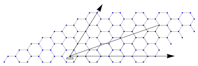
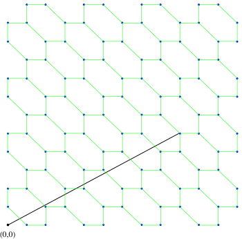
Figure 8. The free path length in the honeycomb and in the deformed honeycomb

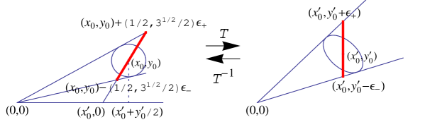
Figure 9. Change of scatterers under the linear transformation $T$

$T$ also maps circular scatterers $(q+\frac{a}{2},\frac{a\sqrt{3}}{2})+\varepsilon(\cos\theta,\sin\theta)$ centered at $(x_{0},y_{0})=(q+\frac{a}{2},\frac{a\sqrt{3}}{2})$ to ellipsoidal scatterers $(q,a)+\varepsilon(\cos\theta-\frac{\sin\theta}{\sqrt{3}},\frac{2\sin\theta}{\sqrt{3}})$ centered at $(x_{0}^{\prime},y_{0}^{\prime})=(q,a)$. Denote $\omega_{0}=\arctan\frac{y_{0}}{x_{0}}$ and $\omega_{0}^{\prime}=\arctan\frac{y_{0}^{\prime}}{x_{0}^{\prime}}$. Denote also $S_{\varepsilon}=\{\delta(\cos\frac{\pi}{3},\sin\frac{\pi}{3}):|\delta|\leqslant\varepsilon\}$.

In the honeycomb with scatterers $\{(x_{0},y_{0})+S_{\varepsilon}:(x_{0},y_{0})\in\Gamma_{+}^{\,\operatorname{hex}}\}$ of same length, the ”local” repartition function

$$\tilde{\mathbb{G}}^{\,\operatorname{hex}}_{I,\varepsilon}(\lambda)=\bigg{|}\bigg{\{}\omega\in\arctan I:\tilde{q}^{\,\operatorname{hex}}_{\varepsilon}(\omega)>\frac{\lambda}{\varepsilon}\bigg{\}}\bigg{|},\qquad I\subseteq\bigg{[}0,\frac{\pi}{6}\bigg{]}\ \ \mbox{\rm interval,}$$ (5.1)

of the ”horizontal” free path length

$$\tilde{q}_{\varepsilon}^{\,\operatorname{hex}}(\omega)=\inf\left\{q\in\mathbb{N}:\exists a\in\mathbb{N},\exists(x_{0},y_{0})\in\Gamma_{+}^{\,\operatorname{hex}},\bigg{(}\frac{q+a/2}{\cos\omega},\frac{a\sqrt{3}/2}{\sin\omega}\bigg{)}\in(x_{0},y_{0})+S_{\varepsilon}\right\},$$

turns out to be closely related with ${\mathbb{G}}_{3,I,\varepsilon}(\lambda)$, being estimated through the same approximation procedure as for the later when $I\subseteq[0,1]$ is a short interval of length $|I|\asymp\varepsilon^{c}$, $0<\varepsilon<1$. Indeed, the equality

$$T^{-1}(x_{0}^{\prime},y_{0}^{\prime}+\delta)=\Bigg{(}x_{0}^{\prime}+\frac{y_{0}^{\prime}+\delta}{2},\frac{(y_{0}^{\prime}+\delta)\sqrt{3}}{2}\Bigg{)},$$

shows that $T$ maps the oblique scatterer $(x_{0},y_{0})+S_{\varepsilon}$ from the honeycomb onto the vertical scatterer $(x_{0}^{\prime},y_{0}^{\prime})+V_{\varepsilon}$ from the square lattice with $x_{0}^{\prime}\equiv y_{0}^{\prime}\pmod{3}$, and the line through the origin with slope $\frac{y_{0}^{\prime}+\delta}{x_{0}^{\prime}}$ onto the line through the origin with slope $\Phi\big{(}\frac{y_{0}^{\prime}+\delta}{x_{0}^{\prime}}\big{)}$, where $\Phi$ is the bijection

$$\Phi:[0,1]\rightarrow\Bigg{[}0,\frac{\sqrt{3}}{3}\Bigg{]},\qquad\Phi(\mu)=\frac{\mu\sqrt{3}}{2+\mu},\qquad\Phi^{-1}(x)=\frac{2x}{\sqrt{3}-x}.$$

In the process the condition $\tilde{q}_{\varepsilon}^{\,\operatorname{hex}}(\omega)>\frac{\lambda}{\varepsilon}$ above is being replaced by $q_{3,\varepsilon}(\omega^{\prime})>\frac{\lambda}{\varepsilon}$ in the square lattice. The only difference arises from replacing expressions (with $x_{0}^{\prime}=q$, $y_{0}^{\prime}=a$ and $0\leqslant\delta\leqslant\frac{1}{q}$)

$$\arctan\frac{y_{0}^{\prime}+\delta}{x_{0}^{\prime}}-\arctan\frac{y_{0}^{\prime}}{x_{0}^{\prime}}=\frac{\delta}{x_{0}^{\prime}}\cdot\frac{1}{1+\frac{y_{0}^{\prime 2}}{x_{0}^{\prime 2}}}+O\Bigg{(}\frac{\delta^{2}}{x_{0}^{\prime 2}}\Bigg{)}=\frac{\delta q}{q^{2}+a^{2}}+O\Bigg{(}\frac{\delta^{2}}{q^{2}}\Bigg{)}$$

that collect the contribution of angles $\omega$ for ${\mathbb{G}}_{3,I,\varepsilon}(\lambda)$, by

$$\begin{split}\arctan\Phi\Bigg{(}\frac{y_{0}^{\prime}+\delta}{x_{0}^{\prime}}\Bigg{)}-\arctan\Phi\Bigg{(}\frac{y_{0}^{\prime}}{x_{0}^{\prime}}\Bigg{)}&=\arctan\frac{(y_{0}^{\prime}+\delta)\sqrt{3}}{2x_{0}^{\prime}+y_{0}^{\prime}+\delta}-\arctan\frac{y_{0}^{\prime}\sqrt{3}}{2x_{0}^{\prime}+y_{0}^{\prime}}\\ &=\Bigg{(}\frac{(y_{0}^{\prime}+\delta)\sqrt{3}}{2x_{0}^{\prime}+y_{0}^{\prime}+\delta}-\frac{y_{0}^{\prime}\sqrt{3}}{2x_{0}^{\prime}+y_{0}^{\prime}}\Bigg{)}\frac{1}{1+\Big{(}\frac{y_{0}^{\prime}\sqrt{3}}{2x_{0}^{\prime}+y_{0}^{\prime}}\Big{)}^{2}}\\ &=\frac{2x_{0}^{\prime}\delta\sqrt{3}}{(2x_{0}^{\prime}+y_{0}^{\prime})^{2}}\Bigg{(}1+O\bigg{(}\frac{\delta}{2x_{0}^{\prime}+y_{0}^{\prime}}\bigg{)}\Bigg{)}\frac{1}{1+\Big{(}\frac{y_{0}^{\prime}\sqrt{3}}{2x_{0}^{\prime}+y_{0}^{\prime}}\Big{)}^{2}}\\ &=\frac{\delta q\sqrt{3}}{2(q^{2}+aq+a^{2})}+O\Bigg{(}\frac{\delta^{2}}{q^{2}}\Bigg{)}.\end{split}$$

The effect will only be on the main term, where $c_{J}=\int_{J}\frac{dx}{1+x^{2}}$, $J\subseteq[0,1]$, will be replaced by $c_{I}^{\operatorname{hex}}:=\int_{\Phi^{-1}(I)}\frac{\sqrt{3}}{2(1+x+x^{2})}\,dx$, $I\subseteq\big{[}0,\frac{1}{\sqrt{3}}\big{]}$. In this way we obtain, uniformly in $\lambda$ on compacts in $\mathbb{R}_{+}\setminus\{1\}$,

$$\tilde{\mathbb{G}}^{\,\operatorname{hex}}_{I,\varepsilon}(\lambda)=c_{I}^{\operatorname{hex}}G_{3}(\lambda)+O_{\delta}\Big{(}\varepsilon^{-\delta+\theta(c,c_{1})}\Big{)}.$$ (5.2)

The change of variable $x=\Phi(\mu)$ gives

$$c^{\Delta}_{[\tan\omega_{0},\tan\omega_{1}]}=\frac{\sqrt{3}}{2}\int_{\Phi^{-1}(\tan\omega_{0})}^{\Phi^{-1}(\tan\omega_{1})}\frac{dx}{x^{2}+x+1}=\int_{\tan\omega_{0}}^{\tan\omega_{1}}\frac{d\mu}{\mu^{2}+1}=\omega_{1}-\omega_{0}.$$ (5.3)

In this case $\tilde{q}_{\varepsilon}^{\,\operatorname{hex}}(\omega)$ and the free path length $\tilde{\tau}_{\varepsilon}^{\,\operatorname{hex}}(\omega)$ are related (by the rule of Sines) by

$$\tilde{\tau}_{\varepsilon}^{\,\operatorname{hex}}(\omega)=\frac{\sin\frac{2\pi}{3}}{\sin\big{(}\frac{\pi}{3}-\omega\big{)}}\ \tilde{q}_{\varepsilon}^{\,\operatorname{hex}}(\omega)=\frac{\sqrt{3}}{2}\cdot\frac{\tilde{q}_{\varepsilon}^{\,\operatorname{hex}}(\omega)}{\cos\big{(}\frac{\pi}{6}+\omega\big{)}},$$

so that

$$\tilde{\mathbb{P}}^{\,\operatorname{hex}}_{I,\varepsilon}(\lambda):=\bigg{|}\bigg{\{}\omega\in\arctan I:\tilde{\tau}_{\varepsilon}^{\,\operatorname{hex}}(\omega)>\frac{\lambda}{\varepsilon}\bigg{\}}\bigg{|}=\bigg{|}\bigg{\{}\omega\in\arctan I:\tilde{q}^{\,\operatorname{hex}}_{\varepsilon}(\omega)>\frac{2\lambda\cos\big{(}\frac{\pi}{6}+\omega\big{)}}{\varepsilon\sqrt{3}}\bigg{\}}\bigg{|}.$$ (5.4)

Fix $\omega_{I}\in\arctan I$. Using $\big{|}\cos\big{(}\frac{\pi}{6}+\omega\big{)}-\cos\big{(}\frac{\pi}{6}+\omega_{I}\big{)}\big{|}\leqslant|\omega-\omega_{I}|\ll\varepsilon^{c}$, (2.2), and $c_{I}^{\operatorname{hex}}\asymp\varepsilon^{c}$, equalities (5.2) and (5.4) yield

$$\tilde{\mathbb{P}}^{\,\operatorname{hex}}_{I,\varepsilon}(\lambda)=c_{I}^{\operatorname{hex}}G_{3}\Bigg{(}\frac{2\lambda\cos\big{(}\frac{\pi}{6}+\omega_{I})}{\sqrt{3}}\Bigg{)}+O_{\delta}\Big{(}\varepsilon^{2c}+\varepsilon^{-\delta+\theta(c,c_{1})}\Big{)}.$$ (5.5)

Let $\varepsilon_{\pm}=\varepsilon_{\pm}(\omega_{0},\varepsilon)$ as in Figure 9. Consider the case of scatterers $(x_{0},y_{0})+S_{\omega_{0},\varepsilon}$, $(x_{0},y_{0})\in\Gamma_{+}^{\,\operatorname{hex}}$, where $S_{\omega_{0},\varepsilon}$ denotes the segment $\{\delta(\cos\frac{\pi}{3},\sin\frac{\pi}{3}):-\varepsilon_{-}\leqslant\delta\leqslant\varepsilon_{+}\}$. Let $\tilde{\tilde{\tau}}^{\,\operatorname{hex}}_{\varepsilon}(\omega)$ denote the free path length and $\tilde{\tilde{{\mathbb{P}}}}^{\,\operatorname{hex}}_{I,\varepsilon}(\lambda)=|\{\omega\in\arctan I:\tilde{\tilde{\tau}}^{\,\operatorname{hex}}_{\varepsilon}(\omega)>\frac{\lambda}{\varepsilon}\}|$. Since $|\cos\omega_{\pm}-\cos\omega_{I}|\ll\varepsilon^{c}$ and $\cos(\frac{\pi}{6}+\omega_{I})>\frac{1}{2}$ there exists $C_{1}>0$ such that

$$\varepsilon^{\prime}:=\varepsilon\left(\frac{1}{\cos(\frac{\pi}{6}+\omega_{I})}-C_{1}\varepsilon^{c}\right)\leqslant\varepsilon_{-}\leqslant\varepsilon_{+}\leqslant\varepsilon^{\prime\prime}:=\varepsilon\left(\frac{1}{\cos(\frac{\pi}{6}+\omega_{I})}+C_{1}\varepsilon^{c}\right).$$ (5.6)

The inequalities $\tilde{\tau}^{\Delta}_{\varepsilon^{\prime\prime}}(\omega)\leqslant\tilde{\tilde{\tau}}^{\Delta}_{\varepsilon}(\omega)\leqslant\tilde{\tau}^{\Delta}_{\varepsilon^{\prime}}(\omega)$ and (5.6) combined with formula (5.5) and (2.2) lead to

$$\begin{split}\tilde{\tilde{{\mathbb{P}}}}_{I,\varepsilon}^{\,\operatorname{hex}}(\lambda)&\leqslant\bigg{|}\bigg{\{}\omega\in\arctan I:\tilde{\tau}^{\,\operatorname{hex}}_{\varepsilon^{\prime}}(\omega)>\frac{\lambda}{\varepsilon}\bigg{\}}\bigg{|}\\ &=\Bigg{|}\Bigg{\{}\omega\in\arctan I:\tilde{\tau}^{\,\operatorname{hex}}_{\varepsilon^{\prime}}(\omega)>\frac{\lambda}{\varepsilon^{\prime}\big{(}\cos(\frac{\pi}{6}+\omega_{I})-C_{1}\varepsilon^{c}\big{)}}\Bigg{\}}\Bigg{|}\\ &=\tilde{{\mathbb{P}}}^{\,\operatorname{hex}}_{\varepsilon}\left(\frac{\lambda}{\cos(\frac{\pi}{6}+\omega_{I})-C_{1}\varepsilon^{c}}\right)\\ &=c_{I}^{\operatorname{hex}}G_{3}\left(\frac{2\lambda}{\sqrt{3}}\cdot\frac{\cos(\frac{\pi}{6}+\omega_{I})}{\cos(\frac{\pi}{6}+\omega_{I})-C_{1}\varepsilon^{c}}\right)+O_{\delta}\Big{(}\varepsilon^{2c}+\varepsilon^{-\delta+\theta(c,c_{1})}\Big{)}\\ &=c_{I}^{\operatorname{hex}}G_{3}\left(\frac{2\lambda}{\sqrt{3}}\right)+O_{\delta}\Big{(}\varepsilon^{2c}+\varepsilon^{-\delta+\theta(c,c_{1})}\Big{)},\end{split}$$

and to a similar lower bound for $\tilde{\tilde{{\mathbb{P}}}}_{I,\varepsilon}^{\,\operatorname{hex}}(\lambda)$, and so we get

$$\tilde{\tilde{{\mathbb{P}}}}_{I,\varepsilon}^{\,\operatorname{hex}}(\lambda)=c_{I}^{\operatorname{hex}}G_{3}\left(\frac{2\lambda}{\sqrt{3}}\right)+O_{\delta}\Big{(}\varepsilon^{2c}+\varepsilon^{-\delta+\theta(c,c_{1})}\Big{)}.$$ (5.7)

The trivial inequality $|\tau_{\varepsilon}^{\Delta}(\omega)-\tilde{\tilde{\tau}}_{\varepsilon}^{\Delta}(\omega)|\leqslant 2\varepsilon$ and (5.7) now provide the formula

$${\mathbb{P}}^{\,\operatorname{hex}}_{I,\varepsilon}(\lambda)=c_{I}^{\operatorname{hex}}G_{3}\left(\frac{2\lambda}{\sqrt{3}}\right)+O_{\delta}\Big{(}\varepsilon^{2c}+\varepsilon^{-\delta+\theta(c,c_{1})}\Big{)}$$ (5.8)

for the repartition function ${\mathbb{P}}^{\,\operatorname{hex}}_{I,\varepsilon}(\lambda)=|\{\omega\in\arctan I:\tau_{\varepsilon}^{\,\operatorname{hex}}(\omega)>\frac{\lambda}{\varepsilon}\}|$ of $\varepsilon\tau_{\varepsilon}^{\,\operatorname{hex}}$.

Finally we choose a partition $\big{[}0,\frac{1}{\sqrt{3}}\big{]}=\cup_{j=1}^{N}I_{j}$ with intervals $I_{j}$ of equal size $\frac{1}{N}\asymp\varepsilon^{c}$. Applying (5.8) to each individual interval $I_{j}$ with $c=c_{1}=\frac{1}{8}$ and summing over $j$ we find

$${\mathbb{P}}^{\,\operatorname{hex}}_{[0,1/\sqrt{3}],\varepsilon}(\lambda)=\sum_{j=1}^{N}c_{I_{j}}^{\,\operatorname{hex}}G_{3}\left(\frac{2\lambda}{\sqrt{3}}\right)+O_{\delta}\Big{(}\varepsilon^{\frac{1}{8}-\delta}\Big{)}=\frac{\pi}{6}G_{3}\left(\frac{2\lambda}{\sqrt{3}}\right)+O_{\delta}\Big{(}\varepsilon^{\frac{1}{8}-\delta}\Big{)}.$$ (5.9)

Theorem 2 now follows immediately from (5.9) and obvious symmetry properties of the honeycomb.

References

- [1] F. P. Boca, C. Cobeli, A. Zaharescu, Distribution of lattice points visible from the origin, Comm. Math. Phys., 213 (2000), 433–470.
- [2] F. P. Boca, R. N. Gologan, A. Zaharescu, The statistics of the trajectory of a certain billiard in a flat two-torus, Comm. Math. Phys. 240 (2003), 53–73.
- [3] F. P. Boca, R. N. Gologan, A. Zaharescu, The average length of a trajectory in a certain billiard in a flat two-torus, New York J. Math. (electronic) 9 (2003), 303–330.
- [4] F. P. Boca, A. Zaharescu, On the correlations of directions in the Euclidean plane, Trans. Amer. Math. Soc. 358 (2006), 1797–1825.
- [5] F. P. Boca, A. Zaharescu, The distribution of the free path lengths in the periodic two-dimensional Lorentz gas in the small-scatterer limit, Comm. Math. Phys. 269 (2007), 425–471.
- [6] E. Caglioti, F. Golse, On the distribution of free path lengths for the periodic Lorentz gas III., Comm. Math. Phys. 236 (2003), 199–221.
- [7] E. Caglioti, F. Golse, The Boltzmann-Grad limit of the periodic Lorentz gas in two space dimensions, C. R. Math. Acad. Sci. Paris 346 (2008), no.7-8, 477–482.
- [8] P. Dahlqvist, The Lyapunov exponent in the Sinai billiard in the small scatterer limit, Nonlinearity 10 (1997), 159–173.
- [9] F. Golse, The periodic Lorentz gas in the Boltzamann-Grad limit, Proc. ICM 2006 Madrid, Spain, Vol.III (invited lectures), pp.183–201.
- [10] J. Marklof, A. Strömbergsson, The distribution of free path lengths in the periodic Lorentz gas and related lattice point problems, preprint math.DS 0706.4395, to appear in Ann. of Math.