On the Decay Rate of the False Vacuum

Abstract

The finite size theory of metastability in a quartic potential is developed by the semiclassical path integral method. In the quantum regime, the relation between temperature and classical particle energy is found in terms of the first complete elliptic integral. At the sphaleron energy, the criterion which defines the extension of the quantum regime is recovered. Within the latter, the temperature effects on the fluctuation spectrum are evaluated by the functional determinants method and computed. The eigenvalue which causes metastability is determined as a function of size/temperature by solving a Lamè equation. The ground state lifetime shows remarkable deviations with respect to the result of the infinite size theory.

I. Introduction

The theory of tunneling in a metastable potential has been a widely investigated topic after the seminal works by Langer and Coleman which provided the mathematical basis of the decay processes in statistical physics langer and quantum field theory cole . In the latter the decay rate of false ground states is suitably evaluated by the Euclidean path integral method in the semiclassical approximation laughlin ; miller : the classical particle paths are selected as the solutions of the Euler-Lagrange equations fulfilling some boundary conditions and, around such stationary points, the imaginary time action is expanded up to second order in the quantum fluctuations whose contribution is evaluated by means of the theory of the functional determinants. It is in the spectrum of the fluctuations that lie the origins of metastability schulman . To be specific, take a particle of mass $M$ moving in a nonlinear potential with frequency $\omega$ and negative quartic parameter $\delta$:

$$V(x)=\,{{M\omega^{2}}\over 2}x^{2}-{{\delta}\over 4}x^{4}$$ (1)

Saying $\pm a$ are the positions of the potential maxima, $\delta$ is given by $\delta=\,{M\omega^{2}/a^{2}}$ in units $eV\AA^{-4}$. Let’s set $a=\,1\AA$ throughout the paper. The point $x=\,0$ is a classical ground state but quantum mechanically the particle can penetrate the hills and explore the abysses at $|x|\geq\sqrt{2}a$. To see how it happens, let’s focus on the positive $x-$axis and consider the classical problem after performing a Wick rotation which maps the time from the real to the imaginary axis, $t\rightarrow-i\tau$, and turns the potential upside down as shown in Fig. 1.

Now the classical equation of motion admits a non trivial solution which, in the infinite size formalism, is known as the bounce. In the path integral language, the bounce is given by that path that starts at $(x_{1}=\,0,\,\tau=\,-\infty)$, reaches the escape point at $(x_{2}=\,\sqrt{2}a,\,\tau=\,\tau_{0})$ and bounces back at $(x_{1}=\,0,\,\tau=\,+\infty)$. The canonical bounce solution is therefore $\tau-$ reversal invariant and consistent with the zero energy $E$ motion (see Fig. 1) between the turning points $x_{1},\,x_{2}$. In the latter the path velocity vanishes. As the bounce path has a maximum versus $\tau$ the bounce path velocity has a node, hence the zero mode of the Schrödinger-like stability equation which governs the quantum fluctuations cannot be the ground state affl . In other words, the bounce is a saddle and not a minimum for the Euclidean action. Thus, there must be a fluctuation whose eigenvalue is lower in energy than the zero mode eigenvalue. It is this negative eigenvalue which requires an analytic continuation in the Gaussian integral and ultimately leads to an imaginary square root fluctuation determinant. When multi bounce solutions are taken into account (due to multiple excursions between $x_{1},\,x_{2}$) one finally gets an explicit formula for the semiclassical tunneling rate as given by the imaginary part of the ground state energy. The fact is that such tunneling rate does not depend on the temperature as the whole theory is based on the infinite size, or $E=\,0$, formalism. The questions I want to deal with in this paper are the following: how is the quantum fluctuations spectrum affected by temperature effects in the quantum regime? And, accordingly, to which extent is the particle lifetime shortened? To get quantitative answers a finite size theory of metastability has to be developed. The focus is here on a non dissipative system grabert ; legg .

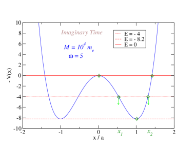
Figure 1: (Color online) Reversed potential of Eq. (1) (units meV). $x_{1}$,$x_{2}$ are the points in which the classical path velocity vanishes. Their location varies with $E$ (in meV). $\omega$ is in meV.

In Section II, I select the family of classical paths which makes stationary the Euclidean action thus generalizing the bounce solution for finite $E$. In Section III, the path integral of the metastable potential is presented together with the solution of the stability equation which governs the quantum fluctuations. The tunneling rate for the finite size theory is calculated in Section IV while the conclusions are drawn in Section V.

II. Finite Size Classical Bounce

In the imaginary time formalism jackiw the particle motion is classically allowed in $-V(x)$ (Fig. 1) as the equation of motion reads:

$$M\ddot{x}_{cl}(\tau)=\,V^{\prime}(x_{cl}(\tau))$$ (2)

where $V^{\prime}$ means derivative with respect to $x_{cl}$. Let’s define

$$\chi_{cl}(\tau)=\,{1\over{\sqrt{2}}}{{x_{cl}(\tau)}\over a}\,$$

$$\kappa=\,{{2E}\over{\delta a^{4}}}$$ (3)

and integrate Eq. (2). Then, one gets:

$$\tau-\tau_{0}=\,\pm{{1\over\omega}}\int_{\chi_{cl}(\tau_{0})}^{\chi_{cl}(\tau)}{{d\chi}\over{\sqrt{-\chi^{4}+\chi^{2}+\kappa/2}}}\,$$

(4)

with integration constant $E$ representing the classical energy associated to the particle motion. In Fig. 1, the potential barrier is sufficiently high to make the semiclassical approximation valid. The center of motion can be set at $\tau_{0}=\,0$ with no loss of generality, then $\tau\in[-L/2,L/2]$ and $L$ is the size of the system, that is the period for a particle excursion to the abyss and back to the starting position. Then the size represents the finite time required for this journey to occur. For negative energies, $-{{\delta a^{4}}\over 4}<E\leq 0$, there are two turning points $x_{1}\,(\chi_{1})$ and $x_{2}\,(\chi_{2})$ ($0\leq x_{1}\leq x_{2}$) which define the bounds for the particle excursion. They are given by:

$$\chi_{1}=\,\sqrt{{1-\sqrt{1+2\kappa}}\over 2}\,{};{}\,\chi_{2}=\,\sqrt{{1+\sqrt{1+2\kappa}}\over 2}$$ (5)

Thus the length of the generalized bounce, $\chi_{2}-\chi_{1}$, depends on $E$ and shrinks from 1 ($E=\,0$) to 0 ($E=\,-V(x=\,a)$) n1 . This marks an essential difference with respect to the bistable $\phi^{4}$ model i1 in which the (anti)instantons interpolates between the two potential minima thereby covering a distance that does not depend on $E$. To integrate Eq. (4) I use the result grad

$$\int_{\chi_{cl}(\tau)}^{\chi_{2}}{d\chi\over{(\chi^{2}-\chi_{1}^{2})(\chi_{2}^{2}-\chi^{2})}}=\,{1\over\chi_{2}}F(\zeta,m)\,$$

$$\zeta=\,\arcsin\Biggl{[}\sqrt{{\chi_{2}^{2}-\chi_{cl}(\tau)^{2}}\over{\chi_{2}^{2}-\chi_{1}^{2}}}\Biggr{]}\,$$

$$m^{2}=\,1-\chi_{1}^{2}/\chi_{2}^{2}$$ (6)

with $F(\zeta,m)$ being the elliptic integral of the first kind with amplitude $\zeta$ and modulus $m$. Then, after setting $\chi_{cl}(\tau_{0})=\,\chi_{2}$, from Eqs. (3), (4), (6) I get the generalized bounce for the finite size theory:

$$x_{cl}(\tau)=\,a\sqrt{2}{{\chi_{2}}{dn(\varpi,m)}}\,$$

$$\varpi=\,{{\chi_{2}\omega(\tau-\tau_{0})}}$$ (7)

where ${dn(\varpi,m)}$ is the Jacobi delta-amplitude defined in Eq. (24). In the $E=\,0$ limit, $m^{2}=\,1$, hence one recovers the bounce solution of the infinite size theory, $x_{cl}(\tau)=\,a\sqrt{2}\cosh^{-1}(\varpi)$. Fig. 2 plots some paths of the family in Eq. (7): the shape of the paths is not essentially modified (with respect to the $E\simeq 0$ path) up to energies of order $|E|\simeq 0.1V(x=a)$. Above this value the bounce progressively shrinks and becomes a point-like object at the sphaleron energy kuznet defined by $E_{sph}\equiv\,|E|=\,V(x=a)$.

$dn(\varpi,m)$ is even function of $\varpi$ in the period $[-K(m),K(m)]$ determined by the first complete elliptic integral $K(m)=\,F(\pi/2,m)$ abram . Then, imposing the boundary conditions on the $\tau-$range, I get from Eq. (7) (with $\tau_{0}=\,0$):

$$\omega L=\,{{2K(m)}\over{\chi_{2}}}$$ (8)

Eq. (8) expresses the fundamental relation between the size $L$ and the particle energy $E$ which is hidden in the modulus according to Eqs. (3), (5) and the last of Eq. (6). Mapping $L$ onto the temperature axis, $L=\,\hbar/(K_{B}T^{*})$ in the spirit of the thermodynamic Bethe Ansatz zamol , one obtains the link between $E$ and the temperature $T^{*}$ at which the particle motion takes place:

$$K_{B}T^{*}=\,{{\hbar\omega}\over 2}{{\chi_{2}}\over{K(m)}}$$ (9)

For $E=\,-V(x=\,a)$, $K(m=\,0)=\,\pi/2$ hence, Eq. (9) leads to the Goldanskii criterion gold for the transition between quantum and activated regime: $K_{B}T_{max}^{*}=\,\hbar\omega/(\sqrt{2}\pi)$. $T_{max}^{*}$ is thus the maximum temperature at which the tunneling occurs. Computation of Eq. (8) shows that $L(|E|)$ is a monotonically decreasing function below the sphaleron energy. This confirms, on general grounds chudno , that the transition at $T_{max}^{*}$ is expected to be a smooth crossover as proposed long time ago affl ; larkin . The physical origin of the smooth change lies in the fact that the bounce is flexible and continuously adapts its shape to the periodic and changeable (with $E$) boundary conditions. Thus the physical picture differs very much from that encountered in studying the bistable $\phi^{4}$ potential i1 ; i2 ; schaefer where the (anti)instantons have to fulfill antiperiodic boundary conditions which are simply imposed by the potential structure. As a consequence the quantum/activated crossover for the bistable $\phi^{4}$ potential is in fact a sharp transition i1 .

The same conclusion regarding the character of the transition at $T_{max}^{*}$ for the metastable $\phi^{4}$ potential may be drawn by a direct evaluation of the classical action $A[x_{cl}]$ which, for the finite size bounce, reads

$$A[x_{cl}]=\,2\sqrt{2M}\int_{x_{1}}^{x_{2}}dx\sqrt{E+V(x)}-E\cdot L$$ (10)

Using Eqs. (1), (7), (8) one can monitor the smooth $E$ (or $T^{*}$) dependence of $A[x_{cl}]$ and its derivative blatter . For $E\rightarrow\,0$, Eq. (10) leads to the infinite size result

$$A[x_{cl}]/\hbar\rightarrow{{4M^{2}\omega^{3}}/({3\hbar\delta}})$$ (11)

The fact that $A[x_{cl}]\propto 1/\delta$ represents the motivation for the semiclassical approach to the quantum tunneling.

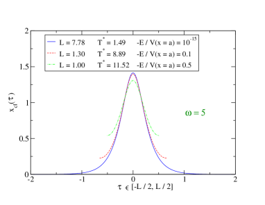
Figure 2: (Color online) Shape of the bounce solution for various classical energies $E$. $L$ is in $sec$ and $T^{*}$ in $K$.

III. Semiclassical Path Integral

The particle path can be written as a sum of the classical background and the quantum fluctuation, $x(\tau)=\,x_{cl}(\tau)+\eta(\tau)$. Then, the semiclassical space-time particle propagator between the positions $x_{i}$ and $x_{f}$ in the imaginary time $L$ is given, in quadratic approximation, by

$$<x_{f}|x_{i}>_{L}=\,\exp\biggl{[}-{1\over{\hbar}}A[x_{cl}]\biggr{]}\cdot\int D\eta\exp\biggl{[}-{1\over{\hbar}}A_{f}[\eta]\biggr{]}\,$$

$$A_{f}[\eta]=\,\int_{-L/2}^{L/2}d\tau{M\over 2}\biggl{(}\dot{\eta}^{2}(\tau)+{1\over M}V^{\prime\prime}(x_{cl}(\tau))\eta^{2}(\tau)\biggr{)}\,$$

$${{V^{\prime\prime}(x_{cl}(\tau))}}=\,M{\omega^{2}}\bigl{(}1-6\chi_{2}^{2}dn^{2}(\varpi,m)\bigr{)}$$ (12)

As $x_{i}$ and $x_{f}$ coincide in our model, Eq. (12) is the single bounce contribution $Z_{1}$ to the total partition function which determines the tunneling rate. Let’s evaluate it. The measure $D\eta$ of the path integration is given through the coefficients $\varsigma_{n}$ of the fluctuation expansion in a series of ortonormal components $\eta_{n}(\tau)$:

$$\int D\eta=\,\aleph\prod_{n=\,0}^{\infty}\int_{-\infty}^{\infty}{{d\varsigma_{n}}\over{\sqrt{2\pi\hbar/M}}}\,$$

$$\eta(\tau)=\,\sum_{n=\,0}^{\infty}\varsigma_{n}\eta_{n}(\tau)$$ (13)

The normalization constant $\aleph$ accounts for the Jacobian in the transformation to the normal mode expansion and the components $\eta_{n}(\tau)$ n3 are the eigenstates (whose eigenvalues are denoted by $\varepsilon_{n}$) of the Schrödinger-like equation:

$$\Bigl{[}-{{d^{2}}\over{d\tau^{2}}}+{{V^{\prime\prime}(x_{cl}(\tau))}\over M}\Bigr{]}\eta_{n}(\tau)=\,\varepsilon_{n}\eta_{n}(\tau)$$ (14)

Supposed to have solved Eq. (14) (see below), after performing Gaussian integrations over the directions $\varsigma_{n}$, one formally obtains the quantum fluctuations factor:

$$\int D\eta\exp\biggl{[}-{1\over{\hbar}}A_{f}[\eta]\biggr{]}=\,{\aleph\Bigl{(}Det[\hat{O}]\Bigr{)}^{-1/2}}\,$$

$$Det[\hat{O}]\equiv\,\prod_{n=\,0}^{\infty}\varepsilon_{n}\,;{}\,\hat{O}\equiv\,-\partial_{\tau}^{2}+{{V^{\prime\prime}(x_{cl})}\over M}$$ (15)

There is however a trouble in Eq. (15) due to the zero eigenvalue $\varepsilon_{0}$ which breaks the Gaussian approximation making $Det[\hat{O}]^{-1/2}$ divergent. It can be easily seen schulman that the zero mode is n4 the path velocity $\dot{x}_{cl}(\tau)$ which solves the Euler-Lagrange problem and the homogeneous differential equation associated to the Eq. (14). The physical origin of the zero mode lies in the fact that the center of motion $\tau_{0}$ of the periodic bounce solutions can be placed everywhere in the range $[-L/2,L/2]$. This mirrors the $\tau$-translational invariance of the system. Then the zero eigenvalue can be extracted from $Det[\hat{O}]$ and, resorting to the integration over $\varsigma_{0}$ in Eq. (13), it can be replaced in Eq. (15) according to the recipe: $(\varepsilon_{0})^{-1/2}\rightarrow\sqrt{{{A[x_{cl}]}\over{2\pi\hbar}}}L$ schulman ; n4a .

A. Functional Determinant

Now I proceed invoking the theory of the functional determinants gelfand ; forman ; cole1 ; kirsten1 ; burgh ; lesch to compute the whole fluctuation contribution embodied in the regularized determinant $Det^{R}[\hat{O}]$ such that $Det[\hat{O}]\equiv\varepsilon_{0}\cdot Det^{R}[\hat{O}]$. The form of $Det^{R}[\hat{O}]$ depends on the type of boundary conditions fulfilled by the quantum fluctuations $\eta_{n}(\tau)$ and their derivatives. To establish it, remember that $\dot{x}_{cl}(\tau)$ is a quantum fluctuation whose periodicity can be promptly checked by deriving Eq. (7):

$$\dot{x}_{cl}(\tau)=\,-a\omega\sqrt{2}m^{2}\chi_{2}^{2}sn(\varpi,m)cn(\varpi,m)\,$$

$$\ddot{x}_{cl}(\tau)=\,-a\omega^{2}\sqrt{2}m^{2}\chi_{2}^{3}dn(\varpi,m)\bigl{[}1-2sn^{2}(\varpi,m)\bigr{]}\,$$

(16)

with the Jacobian elliptic functions $sn(\varpi,m)$ and $cn(\varpi,m)$ defined in Eq. (24). Then, for any two points such that $\varpi_{2}=\varpi_{1}\mp 2K(m)$, one infers that: $\dot{x}_{cl}(\varpi_{2})=\,\dot{x}_{cl}(\varpi_{1})$ and $\ddot{x}_{cl}(\varpi_{2})=\,\ddot{x}_{cl}(\varpi_{1})$. Thus, periodic boundary conditions (PBC) apply to our problem.

In fact, being a product over an infinite number of eigenvalues whose modulus is larger than one, $Det^{R}[\hat{O}]$ is (exponentially) divergent in the $L\rightarrow\infty$ limit whereas ratios of functional determinants are finite and physically meaningful both in value and sign gelfand ; kleinert . Therefore ${Det^{R}[\hat{O}]}$ has to be normalized over the harmonic oscillator determinant ${Det[\hat{h}]}$ with $\hat{h}\equiv\,-\partial^{2}_{\tau}+\omega^{2}$. For any two points separated (as above) by $2K(m)$, the latter corresponding to the period $L$ along the $\tau-$axis, the determinants ratio is formed in the case of PBC by kleinert1 :

$${Det[\hat{h}]} = \,-4\sinh^{2}(\omega L/2)\,$$

$${{Det^{R}[\hat{O}]}\over{<f_{0}|f_{0}>}} = \,{{f_{1}(\varpi_{2})-f_{1}(\varpi_{1})}\over{{f_{0}(\varpi_{1})W(f_{0},f_{1})}}}\,$$

$$f_{1} = \,{{\partial{x}_{cl}(\tau)}\over{\partial m}}\,\,$$

$$f_{0} = \,\dot{x}_{cl}(\tau)\,{}\,$$ (17)

where $f_{0}$, $f_{1}$ are independent solutions of the homogeneous equation associated to Eq. (14), $W(f_{0},f_{1})$ is their Wronskian and $<f_{0}|f_{0}>$ is the squared norm which can be computed by the first in Eq. (16).

Working out the analytical calculation for the second in Eq. (17), I find:

$${{Det^{R}[\hat{O}]}\over{<f_{0}|f_{0}>}}=\,{{(2-m^{2})^{7/2}}\over{a^{2}\omega^{3}m^{4}}}\Biggl{[}{{E(\pi/2,m)}\over{1-m^{2}}}-K(m)\Biggr{]}$$ (18)

where $E(\pi/2,m)$ is the complete elliptic integral of the second kind. As the squared norm has dimension $[\omega a^{2}]$, $Det^{R}[\hat{O}]$ correctly carries the dimension $[\omega^{-2}]$ consistently with the fact that $Det[\hat{O}]$ is dimensionless.

In the $E\rightarrow 0$ ($L\rightarrow\infty$) limit, $m^{2}\rightarrow 1$ and $K(m)\sim\ln(4/\sqrt{1-m^{2}})$. Moreover, $<f_{0}|f_{0}>\sim{4\over 3}\omega a^{2}$.

Then, from Eqs. (17), (18), in the same limit, I get

$${{Det[\hat{h}]}\over{Det^{R}[\hat{O}]}}\rightarrow\,-{{12\omega^{2}}}$$ (19)

Thus recovering the well known result of the infinite size bounce theory. In fact this occurs quite away from the zero limit as clearly shown in Fig. 3 where the determinants ratio (normalized over $-12\omega^{2}$) is plotted against $T^{*}$ obtained from Eq. (9). As $\omega=\,5meV$, $T_{max}^{*}$ is set here at $\sim 13K$ although it may be much larger in real systems hanggi . The result of Eq. (19) is already achieved at $T^{*}\sim 7K$, that is about the value at which the finite size bounce fits the infinite size bounce (see Fig. 2). This looks remarkable as it suggests that quantum fluctuations and classical path start to experience the finite size effects starting from the same temperature. In the $T^{*}\rightarrow 0$ limit, computation of Eq. (18) becomes time consuming in order to control the elliptic integrals and reproduce the exponential divergence due to the $(1-m^{2})^{-1}$ term.

The negative sign in Eq. (19) is crucial and occurs for any $T^{*}$. Then, the square root of the determinant ratio (which appears in the partition function) is imaginary. As stated at the beginning and made clear in Fig. 2 the bounce has always a maximum hence, the zero mode is not the ground state: there is a negative eigenvalue $\varepsilon_{-1}$ n5 embedded in $Det^{R}[\hat{O}]$ which causes a finite lifetime for the particle placed at $x=\,x_{1}$. While such eigenvalue is easily found ($\varepsilon_{-1}=\,-3\omega^{2}$) in the infinite size theory as the operator in the l.h.s. of Eq. (14) becomes of Rosen-Morse type landau , here I am facing a non trivial problem: that to determine $\varepsilon_{-1}$ at finite $E$ and establish its effect in the temperature dependence of the particle lifetime.

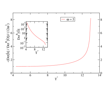
Figure 3: (Color online) Normalized determinants ratio versus $T^{*}(K)$. The inset plots the regularized fluctuation determinant (units $meV^{-2}$) of Eq. (18).

B. Lamè equation

To pursue this goal, insert the last of Eqs. (12) in the stability equation  (14) which easily transforms into:

$${{d^{2}}\over{d\varpi^{2}}}\eta_{n}(\tau)=\,\bigl{[}l(l+1)m^{2}sn^{2}(\varpi,m)+\mathcal{A}_{n}\bigr{]}\eta_{n}(\tau)\,$$

$$\mathcal{A}_{n}=\,{1\over{\chi_{2}^{2}}}-l(l+1)-{{\varepsilon_{n}}\over{(\chi_{2}\omega)^{2}}}\,$$

$$l(l+1)=\,6$$ (20)

This is the Lamè equation in the Jacobian form whittaker that, for given $l$ and $m$, admits periodic solutions (which can be expanded in infinite series) for an infinite sequence of characteristic $\mathcal{A}_{n}$ values. The continuum of the fluctuation spectrum stems from this sequence. However, for positive and integer $l$, (in the case at hand, $l=\,2$), the first $2l+1$ solutions of Eq. (20) are not infinite series but polynomials in the Jacobi elliptic functions with real period $2K(m)$ or $4K(m)$ ward . $2K(m)$ plays the role of the lattice constant being the period of the potential in the Schrödinger like stability equation. It is among these five polynomial solutions corresponding to the eigenvalues $\mathcal{A}_{n}$ that one has to pick up the unstable fluctuation eigenstate. Two solutions out of five have to be discarded because they do not fulfill the periodicity conditions required for the fluctuation components: $\eta_{n}(\varpi)=\,\eta_{n}(\varpi\mp 2K(m))$. The three (unnormalized) good solutions are i3 :

$$\eta_{-1}\propto\,sn^{2}(\varpi,m)-{1\over{1+m^{2}-\sqrt{m^{4}-m^{2}+1}}}\,$$

$$\eta_{0}\propto\,sn(\varpi,m)cn(\varpi,m)\,$$

$$\eta_{1}\propto\,sn^{2}(\varpi,m)-{1\over{1+m^{2}+\sqrt{m^{4}-m^{2}+1}}}\,$$

(21)

and, using Eqs. (20), I get the corresponding energy bands $\varepsilon_{n}$ as functions of the modulus $m$:

$$\varepsilon_{-1}=\,-\omega^{2}\Biggl{(}1+{2\over{2-m^{2}}}\sqrt{m^{4}-m^{2}+1}\Biggr{)}\,$$

$$\varepsilon_{0}=\,0\,$$

$$\varepsilon_{1}=\,-\omega^{2}\Biggl{(}1-{2\over{2-m^{2}}}\sqrt{m^{4}-m^{2}+1}\Biggr{)}$$ (22)

The zero mode is thus consistently recovered also for the finite size theory with $\eta_{0}\propto\dot{x}_{cl}$ n4 . $\eta_{1}$ lies in the continuum with $\varepsilon_{1}\rightarrow\omega^{2}$ in the infinite size limit. $\varepsilon_{-1}$ is the object of our focus. Through Eqs. (5), (6) and  (9), the $T^{*}$ dependence of $\varepsilon_{-1}$ is computed as shown in the inset of Fig. 4: the value $-3\omega^{2}$ of the infinite size theory is mantained up to $T^{*}\sim 7K$ while $|\varepsilon_{-1}|$ softens significantly at larger $T^{*}$. This strongly affects the overall behavior of $Det^{R}[\hat{O}]$ as I point out by plotting the ratio $Det^{R}[\hat{O}]/\varepsilon_{-1}$ on a linear scale.

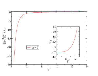
Figure 4: (Color online) Ratio (in $meV^{-4}$) between the regularized fluctuation determinant and the ground state eigenvalue versus temperature. The inset plots separately the $T^{*}$ dependence of the g.s. eigenvalue (in $meV^{2}$).

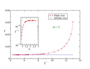
Figure 5: (Color online) Tunneling rate (in $meV$) computed from Eq. (23) versus temperature. The rate of the infinite size theory is plotted for comparison. The inset shows the lifetime (in $sec$) against the size $L$.

IV. Decay Rate

All the ingredients are now available to compute Eq. (12) and derive the total partition function $Z_{T}$. Note that also the solution of Eq. (2), $x_{cl}=\,0$ contributes with a term $Z_{h}$ to $Z_{T}$. Being $Z_{h}=\,\aleph|Det[\hat{h}]|^{-1/2}$, we now fully understand on physical grounds the need to normalize $Det^{R}[\hat{O}]$ over $Det[\hat{h}]$ as described above. In fact, one has to account for all multiple excursions to and from the abyss which is equivalent to sum over an infinite number of (non interacting) bounce contributions as $Z_{1}$ in Eq. (12). The final result is: $Z_{T}=\,Z_{h}\exp(Z_{1}/Z_{h})$. The tunneling rate $\Gamma(L)$ is thus obtained from the imaginary part of the exponent in $Z_{T}$ ($Z_{1}$ is purely imaginary) through the Feynman-Kac formula schulman . The general expression for a finite size system is:

$$\Gamma(L)=\,\hbar\sqrt{{{A[x_{cl}]+E\cdot L}\over{2\pi\hbar}}}\sqrt{{{Det[\hat{h}]}\over{Det^{RR}[\hat{O}]\bigl{|}\varepsilon_{-1}\bigl{|}}}}\exp\biggl{[}-{1\over{\hbar}}A[x_{cl}]\biggr{]}\,$$

(23)

with $Det^{RR}[\hat{O}]\equiv\,Det^{R}[\hat{O}]/\varepsilon_{-1}$ being negative as shown in Fig. 4. Eq. (23) is plotted in Fig. 5 against $T^{*}$ together with the constant tunneling rate of the infinite size theory. $\Gamma(T^{*})$ grows fast as the length of the bounce shrinks and the quantum fluctuations spectrum softens. Close to $T_{max}^{*}$, the tunneling rate has increased by an order of magnitude with respect to the infinite size result but the decay width remains smaller than the fundamental oscillator energy being $\Gamma(T^{*}=\,12.98K)/\omega\sim 6\cdot 10^{-3}$. The inset in Fig. 5 plots the lifetime of the false vacuum versus the system size.

V. Conclusion

This work presents a study of the finite size effects on a metastable quartic nonlinear potential and, as such, is complementary to a previous investigation i1 . The semiclassical path integral method, implemented by the theory of the functional determinants, builds the framework to analyse the tunneling in the metastable system. The description relies on the properties of the elliptic functions which permit to monitor the evolution of the classical bounce versus the system size. After defining the temperature range within which the tunneling occurs, I have computed the temperature effects on the quantum fluctuation spectrum. In particular, the negative eigenvalue which causes metastability has been studied in great detail solving a Lamè type equation. These results, new in the literature, permit to compute the physical properties of the false ground state. Specifically I have shown that its lifetime has a remarkable size/temperature dependence inside the quantum regime. While the latter can persist up to $T_{max}^{*}$ of order $100K$ in real systems, the presented quantitative method may also be of practical interest provided the potential parameters are adapted to specific cases.

*

Appendix A

The Jacobian elliptic functions used throughout the paper are related to the amplitude $\zeta$ in Eq. (6) by the definitions

$$sn(\varpi,m)=\,\sin\zeta\,$$

$$cn(\varpi,m)=\,\cos\zeta\,$$

$$dn(\varpi,m)=\,\sqrt{1-m^{2}\sin^{2}\zeta}$$ (24)

In the computation of the bounce and its time derivative, the following representations as trigonometric series have been used grad

$$sn(\varpi,m)=\,{{2\pi}\over{mK(m)}}\sum_{n=1}^{\infty}{{q^{n-1/2}}\over{1-q^{2n-1}}}\sin\Bigl{(}{{(2n-1)\pi\varpi}\over{2K(m)}}\Bigr{)}\,$$

$$cn(\varpi,m)=\,{{2\pi}\over{mK(m)}}\sum_{n=1}^{\infty}{{q^{n-1/2}}\over{1+q^{2n-1}}}\cos\Bigl{(}{{(2n-1)\pi\varpi}\over{2K(m)}}\Bigr{)}\,$$

$$dn(\varpi,m)=\,{{\pi}\over{2K(m)}}+{{2\pi}\over{K(m)}}\sum_{n=1}^{\infty}{{q^{n}}\over{1+q^{2n}}}\cos\Bigl{(}{{n\pi\varpi}\over{K(m)}}\Bigr{)}\,$$

$$q=\,\exp\bigl{(}-\pi K^{\prime}(m)/K(m)\bigr{)}\,$$

$$K^{\prime}(m)=\,F(\pi/2,\bar{m})\,$$

$$\bar{m}^{2}=\,{1-m^{2}}$$ (25)

with $\varpi$ defined in Eq. (7). Numerical convergence is achieved by taking a cutoff $n_{max}\sim\,40$ in the Fourier series.

References

- (1) J.S.Langer, Ann. Phys. 41, 108 (1967).
- (2) S.Coleman, Phys. Rev. D 15, 2929 (1977); C.G.Callan and S.Coleman, Phys. Rev. D 16, 1762 (1977).
- (3) D.McLaughlin, J.Math.Phys. 13, 1099 (1972).
- (4) W.H.Miller, J.Chem.Phys. 62, 1899 (1975).
- (5) L.S.Schulman, Techniques and Applications of Path Integration (Wiley&Sons, New York, 1981).
- (6) I.Affleck, Phys. Rev. Lett. 46, 388 (1981).
- (7) H.Grabert, P.Olschowski and U.Weiss, Phys. Rev. B 36, 1931 (1987).
- (8) A.J.Leggett, S.Chakravarty, A.T.Dorsey, M.P.A.Fisher, A.Garg and W.Zwerger, Rev. Mod. Phys. 59, 1 (1987).
- (9) R.Jackiw, Rev.Mod.Phys. 49, 681 (1977).
- (10) Note that the classical problem admits a solution also for positive up to the sphaleron energy . However, in this case there would be only one turning point located at . Thus the particle would explore portions of the abyss which become broader by increasing .
- (11) M.Zoli, J.Math.Phys. 48, 012111 (2007).
- (12) I.S.Gradshteyn and I.M.Ryzhik, Tables of Integrals, Series and Products (Academic Press, New York, 1965) .
- (13) A.N.Kuznetsov and P.G.Tinyakov, Phys.Lett.B 406, 76 (1997).
- (14) M.Abramowitz and I.A.Stegun, Handbook of Mathematical Functions, (Dover Publications, New York, 1972).
- (15) A.Zamolodchikov, J.Phys.A:Math.Gen. 39, 12863 (2006).
- (16) V.I.Goldanskii, Sov.Phys.Dokl. 4, 74 (1959).
- (17) E.M.Chudnovski, Phys. Rev. A 46, 8011 (1992).
- (18) A.I.Larkin and Y.N.Ovchinnikov, Sov.Phys.JETP 59, 420 (1984).
- (19) Sometimes the term ”instanton” is misleadingly used to denote also the ”bounce” solution. The different boundary conditions fulfilled by the two objects underlie profound differences in their dynamics. The former interpolates between the potential minima going across the barrier (the valley in the reversed potential) nearly instantaneously and with finite velocity, hence it spends a very short time around its center of motion . The latter starts from the false vacuum, travels through the barrier and reaches the edge of the abyss at . There it stops, inverts the motion and goes back to the initial position. Then, the Goldstone modes related to the instanton and bounce trajectories have zero and one node respectively.
- (20) T.Schäfer and E.V.Shuryak, Rev.Mod.Phys. 70, 323 (1998).
- (21) D.A.Gorokhov and G.Blatter, Phys. Rev. B 56, 3130 (1997).
- (22) The dimensionalities are: , , .
- (23) The path velocity is proportional to the zero mode fluctuation and is the squared norm used in Eq. (17).
- (24) Precisely, the replacement is: which tends to the expression in the text for the limit.
- (25) I.M.Gelfand and A.M.Yaglom, J.Math.Phys. 1, 48 (1960).
- (26) R.Forman, Invent.Math. 88, 447 (1987).
- (27) S.Coleman, Aspects of Symmetry: Selected lectures of Sidney Coleman (CUP, Cambridge, 1985).
- (28) K.Kirsten and A.J.McKane, Ann. Phys. 308, 502 (2003); ibid. J.Phys A:Math.Gen. 37, 4649 (2004).
- (29) D.Burghelea, L.Friedlander and T.Kappeler. Commun. Math. Phys. 138, 1 (1991).
- (30) M.Lesch, Math. Nachr. 194, 139 (1998).
- (31) H.Kleinert, Path Integrals in Quantum Mechanics, Statistics, Polymer Physycs and Financial Markets (World Scientific Publishing, Singapore, 2004).
- (32) P.Hänggi, P.Talkner and M.Borkovec, Rev. Mod. Phys. 62, 251 (1990).
- (33) H.Kleinert and A.Chervyakow, Phys.Lett.A 245, 345 (1998).
- (34) In Eq. (13) and following the sums and products run over . To be precise they all contain also the negative eigenvalue formally defined by .
- (35) L.D.Landau, E.M.Lifshitz, Quantum Mechanics ed. (Butterworth-Heinemann, Oxford, 1977).
- (36) E.T.Whittaker and G.N.Watson, A Course of Modern Analysis ed. (Cambridge University Press, 1927).
- (37) R.S.Ward, J.Phys.A: Math.Gen. 20, 2679 (1987).
- (38) Note that the way to order eigenvalues and eigenstates in terms of is purely conventional. Either or can be used. The former is assumed consistently with having labelled the unstable eigenvalue by . See n5 .