Spin-polarized current and shot noise in the presence of spin flip in a quantum dot via nonequilibrium Green’s functions

Abstract

Using non-equilibrium Green functions we calculate the spin-polarized current and shot noise in a ferromagnet–quantum-dot–ferromagnet (FM-QD-FM) system. Both parallel (P) and antiparallel (AP) magnetic configurations are considered. Coulomb interaction and coherent spin-flip (similar to a transverse magnetic field) are taken into account within the dot. We find that the interplay between Coulomb interaction and spin accumulation in the dot can result in a bias-dependent current polarization $\wp$. In particular, $\wp$ can be suppressed in the P alignment and enhanced in the AP case depending on the bias voltage. The coherent spin-flip can also result in a switch of the current polarization from the emitter to the collector lead. Interestingly, for a particular set of parameters it is possible to have a polarized current in the collector and an unpolarized current in the emitter lead. We also found a suppression of the Fano factor to values well below 0.5.

year number number identifier Date: ]

I INTRODUCTION

Spin-dependent transport in quantum dots is a subject of intense study nowdays due to its relevance to the new generation of proposed spintronic devices that encompasses, for instance, the Datta-Das transistor,dattadas memory devicessc02 ; mk04 and as an ultimate goal quantum computers.dda02 In particular, the recent progress in the coherent control of electron spins in quantum dots jme04 ; acj05 ; fhlk06 has stimulated even further the research in this field, for possible applications in quantum computation and quantum information processing.man00 In addition to these fascinating technological applications, quantum dots constitute a unique well-controllable system to study fundamental physical aspects of transport in the strong Coulomb-correlated regime, and its interplay with spin-dependent effects.

A common geometry used for transport studies in quantum dots consists of two leads weakly coupled to a quantum dot (QD) via tunneling barriers. Spin-dependent effects such as spin accumulation and spin-polarized transport can occur in these systems when both leads are (or at least one of them is) ferromagnetic (FM). The junction FM-QD-FM resembles the standard TMR mj75 ; jsm95 and GMR mnb88 geometries composed of an insulator layer sandwiched by two ferromagnetic metallic leads, except for the quantum dot replacing the insulator layer. This system (dot coupled to FM leads) was recently experimentally realized in the context of semiconductor quantum dotskh07_1 ; kh07_2 and molecules.anp04 ; ss05 ; cam07 A wealth of novel spin-dependent effects has been observed in this system due to the interplay of quantum confinement, Coulomb correlations, Pauli principle and lead-polarization alignments. For instance, novel effects such as spin-accumulation,iw06 ; iw05 spin-diode,fms07_1 ; commentNina spin-blockade,fe06 ; ac04 ; ac04_2 ; mp03 spin-current ringing,fms07_3 ; ep08 negative differential conductance and negative TMR,fe06 ; iw06 and so on, arise in this context. In order to obtain additional information, not contained in the average current, shot noise has also been analyzed in several spintronic systems. A few exemples include shot noise in spin-valve junctionsbrb99 ; yt01 ; egm03 ; mz05 and quantum dots attached to ferromagnetic leads.rl03 ; fms02 ; du07

Here we apply the Keldysh non-equilibrium technique to study spin-polarized transport (current and shot noise) in a FM-QD-FM system (Fig. 1). Both parallel (P) and antiparallel (AP) lead magnetization alignments are considered. The left and the right lead materials are taken to be different, thus resulting in additional effects, not seen for leads with the same material. We analyze both the current and the shot noise in the presence of Coulomb interaction and spin-flip in the dot. We find an interplay between spin accumulation and Coulomb interaction that gives rise to a bias dependent current polarization $\wp$. More specifically, $\wp$ can be suppressed or enhanced and have its sign changed, depending on the magnetic alignment and the bias voltage. We also note that the spin-flip can switch the current polarization as it flows from the emitter to the collector lead. In particular, it is possible to have an unpolarized emitter-current and a polarized collector-current. For the shot noise, we find that spin-flip can suppress it (in the AP case) with Fano factors reaching well below 1/2.

The outline of our paper is as follows. In Sec. II we describe in detail our model Hamiltonian. In Sec. III we present the current and the noise calculations, respectively, including general formulas for these quantities. In Sec. IV we present and discuss numerical results for the current and the shot noise. We summarize our conclusions in Sec. V. Technical details of our calculation are described in the appendixes A-D.

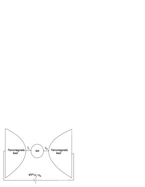
Figure 1: Schematic of the system studied: a quantum dot coupled to two ferromagnetic leads. On the forward bias the electrons tunnel from the left lead to the right lead via the quantum dot. We consider configurations in which the FM leads are parallel (P) or antiparallel (AP). The dot has a single orbital level and can hold at most two electrons of opposite spins. Intradot Coulomb interaction and spin-flip are considered.

II Model system and Hamiltonian

Our system consists of a quantum dot with one quantized level coupled to two ferromagnetic leads via tunneling barriers. While the electrons in the leads are noninteracting, the electrons in the dot experience Coulomb repulsion and spin-flip scattering. The system Hamiltonian is

$$H=H_{L}+H_{R}+H_{D}+H_{T}.$$ (1)

The first three terms in (1) correspond to the three different regions: left lead, right lead and dot. The last term $H_{T}$ hybridizes these three regions thus allowing electrons to tunnel from one region to the other. This term gives rise to current in the presence of a bias voltage.

More explicitly, we have for the ferromagnetic leads

$$H_{\eta}=\sum_{k\sigma}\epsilon_{k\sigma\eta}c_{k\sigma\eta}^{\dagger}c_{k\sigma\eta},$$ (2)

where $\epsilon_{k\sigma\eta}=\epsilon_{k\eta}+(-1)^{\delta_{\sigma\downarrow}}\Delta$ (Stoner Model) is the spin-dependent energy of the electron in lead $\eta=(L,R)$, with the band spin splitting $\Delta$, $\sigma=\uparrow,\downarrow$ and $\delta_{\uparrow\uparrow(\downarrow\downarrow)}=1$, $\delta_{\downarrow\uparrow(\uparrow\downarrow)}=0$. The operator $c_{k\sigma\eta}$ $(c_{k\sigma\eta}^{\dagger})$ destroys (creates) an electron with wave vector $k$ and spin $\sigma$ in lead $\eta$. The dot Hamiltonian is

$$H_{D}=\sum_{\sigma}\epsilon_{\sigma}d_{\sigma}^{\dagger}d_{\sigma}+Un_{\uparrow}n_{\downarrow}+R(d_{\uparrow}^{\dagger}d_{\downarrow}+d_{\downarrow}^{\dagger}d_{\uparrow}),$$ (3)

where $\epsilon_{\sigma}$ is the dot level and $d_{\sigma}$ $(d_{\sigma}^{\dagger})$ annihilates (creates) an electron in the dot with spin $\sigma$. Our model assumes a single spin-degenerate orbital level in the dot, $\epsilon_{\uparrow}=\epsilon_{\downarrow}=\epsilon$. More specifically, our dot can be singly occupied by an electron with spin up or down or doubly occupied by two electrons with opposite spins. We account for the Coulomb interaction in the dot via the Hubbard term with correlation parameter $U$. We assume a linear voltage drop across the system: $\epsilon=\epsilon_{0}-\frac{eV}{2}$, where $e>0$, $V$ is the applied voltage and $\epsilon_{0}$ is the dot level for $V=0$. The left $\mu_{L}$ and the right $\mu_{R}$ chemical potentials are related by $\mu_{L}-\mu_{R}=eV$. Here we assume that $\mu_{L}$ is constant and defines the origin of the energy. For positive bias ($\mu_{L}>\mu_{R}$) the left lead is the electron emitter and the right lead is the collector. The last term in (3) accounts for a coherent spin-flip in the dot.footR This term can represent, e.g., a local transverse magnetic field that coherently rotates the electron spin, which can be experimentaly realized via ESR techniqueshe01 or by the Hanle effect.hanle ; mb05

Instead of carrying out the calculations with the Hamiltonian (3), we perform the following canonical transformation,

$$d_{\sigma}=\frac{1}{\sqrt{2}}\sum_{i=1,2}(-1)^{i\delta_{\sigma\downarrow}}d_{i}.$$ (4)

With (4), the dot Hamiltonian becomes

$$H_{D}=\sum_{i=1,2}[\epsilon_{0}+(-1)^{i}R]d_{i}^{\dagger}d_{i}+Un_{1}n_{2},$$ (5)

where $n_{i}=d_{i}^{\dagger}d_{i}$. Note that in (5) the dot level is split into two levels; $\epsilon_{1}=\epsilon_{0}-R$ and $\epsilon_{2}=\epsilon_{0}+R$. We note that this canonical transformation rotates the spin quantization axis (e.g., to the direction of a local transverse magnetic field), thus replacing the spin-flip term by a diagonal term with a split level.

The tunneling Hamiltonian in (1) is

$$H_{T}=\sum_{k\sigma\eta}(t_{k\sigma}c_{k\sigma\eta}^{\dagger}d_{\sigma}+t_{k\sigma}^{*}d_{\sigma}^{\dagger}c_{k\sigma\eta}),$$ (6)

where the matrix element $t_{k\sigma}$ connects an electronic state in lead $\eta$ to one in the dot. Observe that the hopping process between the leads and the dot is spin conserving, i.e., $t_{k\sigma}$ does not mix different spin components. Applying the transformation (4) in (6) we find

$$H_{T}=\sum_{k\sigma\eta i}\frac{(-1)^{i\delta_{\sigma\downarrow}}}{\sqrt{2}}\{t_{k\sigma}^{*}d_{i}^{\dagger}c_{k\sigma\eta}+t_{k\eta\sigma}c_{k\sigma\eta}^{\dagger}d_{i}\}.$$ (7)

Next we calculate current and noise for the model described above.

III Current and Noise

The current is calculated in the standard way from the definition $I_{L}(t)=\langle\hat{I}_{L}(t)\rangle$ where $\widehat{I}_{L}(t)=-e\dot{N}_{L}$ is the current operator, with $N_{L}=\sum_{k\sigma}c_{k\sigma L}^{\dagger}c_{k\sigma L}$ being the total number operator, and $\langle...\rangle$ is a thermodynamic average. From the Heisenberg equation $\dot{N_{L}}=i[H,N_{L}]$, we find

$$\hat{I}_{L}(t)=ie\sum_{k\sigma}[t_{k\sigma}c_{k\sigma\eta}^{\dagger}(t)d_{\sigma}(t)-t_{k\sigma}^{*}d_{\sigma}^{\dagger}(t)c_{k\sigma\eta}(t)],$$ (8)

which results in the following current expressionym92 ; apj94

$$I_{L}(t)=2e\mathrm{Re}\sum_{k\sigma}t_{k\sigma}i\langle c_{kL\sigma}^{\dagger}(t)d_{\sigma}(t)\rangle.$$ (9)

A similar expression holds for the right lead current $I_{R}=-e\langle\dot{N}_{R}\rangle$. Since we are in stationary regime we have simply $I_{L}=-I_{R}$. Using the canonical transformation in Eq. (9) we obtain

$$I_{L}=2e\mathrm{Re}\sum_{k\sigma i}t_{k\sigma}\frac{(-1)^{i\delta_{\sigma\downarrow}}}{\sqrt{2}}G_{ik\sigma L}^{<}(t,t),$$ (10)

where $G_{ik\sigma L}^{<}(t,t)=i\langle c_{kL\sigma}^{\dagger}(t)d_{i}(t)\rangle$ is the lesser Green function, which is calculated via the Keldysh nonequilibrium technique.lvk65 ; hh96

As a starting point we construct the complex time Green function $G_{ik\sigma L}(\tau,\tau^{\prime})=-i\langle T_{c}d_{i}(\tau)c_{k\sigma L}^{\dagger}(\tau^{\prime})\rangle$, where $T_{c}$ is the contour time-ordering operator and $\tau$ and $\tau^{\prime}$ are complex times running along a complex contour.lvk65 ; hh96 Then we go from the Heisenberg to the interaction picture, by introducing the $S$-matrix operator $S=e^{-i\int_{c}d\tau\widetilde{H}_{T}(\tau)}$. Here the tilde means that $H_{T}$ is in the interaction picture. After expanding $S$ we find,apj94

$$G_{ik\sigma L}(\tau,\tau^{\prime})=t_{k\sigma}^{*}\sum_{j}\frac{(-1)^{j\delta_{\sigma\downarrow}}}{\sqrt{2}}$$

$$\phantom{xxxxxxxx}\times\int_{c}d\tau_{1}G_{ij}(\tau,\tau_{1})g_{k\sigma L}(\tau_{1},\tau^{\prime}),$$ (11)

where $G_{ij}(\tau,\tau_{1})=-i\langle T_{c}d_{i}(\tau)d_{j}^{\dagger}(\tau_{1})\rangle$ and $g_{k\sigma L}(\tau_{1},\tau^{\prime})=-i\langle T_{c}\widetilde{c}_{k\sigma L}(\tau_{1})\widetilde{c}_{k\sigma L}^{\dagger}(\tau^{\prime})\rangle$. Note that while $G_{ij}(\tau,\tau_{1})$ is in the Heisenberg picture, $g_{k\sigma L}(\tau_{1},\tau^{\prime})$ is in the interaction picture (denoted by the tilded operators). This “separability” of the interaction and Heisenberg pictures follows from the assumption of noninteracting electrons in the leads. This allows us to put the “difficult” part of the analysis entirely in the dot Green functions, which contain the Coulomb interaction, the spin-flip and the coupling to leads.

The next step is to apply Langreth’s analytical continuation rules hh96 to (III), to find the lesser Green function appearing in (10). This yields

$$G_{ik\sigma L}^{<}(t,t^{\prime})=t_{kL\sigma}^{*}\sum_{j}\frac{(-1)^{j\delta_{\sigma\downarrow}}}{\sqrt{2}}\int dt_{1}\times$$

$$\{G_{ij}^{r}(t,t_{1})g_{k\sigma L}^{<}(t_{1},t^{\prime})+G_{ij}^{<}(t,t_{1})g_{k\sigma L}^{a}(t_{1},t^{\prime})\},$$ (12)

where the labels $r$, $a$ and $<$ mean retarded, greater and lesser, respectively. The calculation of the retarded $G_{ij}^{r}$, and lesser $G_{ij}^{<}$ dot Green functions is presented in the Appendix A.

Using this result in (10) we arrive at

$$I_{L} = 2e\mathrm{Re}\sum_{ij}\int dt_{1}$$ (13)

$$\times \{G_{ij}^{r}(t,t_{1})\Sigma_{ji}^{<}(t_{1},t)+G_{ij}^{<}(t,t_{1})\Sigma_{ji}^{a}(t_{1},t)\}$$

where $\Sigma_{ji}^{L(<,a)}(t_{1},t)$=$\frac{1}{2}\sum_{k\sigma}|t_{k\sigma}|^{2}(-1)^{(i+j)\delta_{\sigma\downarrow}}$ $g_{k\sigma L}^{(<,a)}(t_{1},t)$, with the lesser Green function $g^{<}_{k\sigma L}(t_{1},t)=i\langle\widetilde{c}_{k\sigma L}^{\dagger}(t)\widetilde{c}_{k\sigma L}(t_{1})\rangle$, and the advanced one $g_{k\sigma L}^{a}(t_{1},t)=i\theta(t-t_{1})\langle\{\widetilde{c}_{k\sigma L}(t_{1}),\widetilde{c}_{k\sigma L}^{\dagger}(t)\}\rangle$, here the curly brackets denote an anticommutator.

In the steady state regime the Fourier transforms of the Green functions result in single frequency Green functions. Since this is the regime of interest here, we state for later use the Fourier transform of the leads Green functions,

$$g_{k\sigma\eta}^{a}(\epsilon) = g_{k\sigma\eta}^{r^{*}}(\epsilon)=\frac{1}{\epsilon-\epsilon_{k\sigma\eta}-i\delta},$$ (14)

$$g_{k\sigma\eta}^{<}(\epsilon) = 2\pi in_{\eta}(\epsilon)\delta(\epsilon-\epsilon_{k\sigma\eta}),$$ (15)

where $n_{\eta}$ is the Fermi distribution function of lead $\eta$.

III.1 Average current in the stationary regime

In a stationary regime all of the Green functions depend on only $t-t_{1}$, yielding the Fourier transform

$$I_{L} = 2e\mathrm{Re}\int\frac{d\epsilon}{2\pi}\sum_{ij}\{G_{ij}^{r}(\epsilon)\Sigma_{ji}^{L<}(\epsilon)+G_{ij}^{<}(\epsilon)\Sigma_{ji}^{La}(\epsilon)\},$$ (16)

$$= ie\int\frac{d\epsilon}{2\pi}\mathrm{Tr}\{\mathbf{\Gamma}^{L}[(\mathbf{G}^{r}-\mathbf{G}^{a})n_{L}+\mathbf{G}^{<}]\},$$

with

$$\mathbf{\Gamma}^{L}=\frac{1}{2}\left(\begin{array}[]{cc}\Gamma_{\uparrow}^{L}+\Gamma_{\downarrow}^{L}&\Gamma_{\uparrow}^{L}-\Gamma_{\downarrow}^{L}\\ \Gamma_{\uparrow}^{L}-\Gamma_{\downarrow}^{L}&\Gamma_{\uparrow}^{L}+\Gamma_{\downarrow}^{L}\end{array}\right),$$ (17)

where $\Gamma_{\sigma}^{L}=2\pi\sum_{k}|t_{k\sigma}|^{2}\delta(\epsilon-\epsilon_{k\sigma L})$ is the linewidth function. In what follows we neglect the energy-dependence of $\Gamma_{\sigma}^{\eta}$ (wideband limit), which will be taken as a constant phenomenological parameter.

III.2 Spin-resolved currents

From Eqs. (16) and (17) we can also determine the spin-resolved components of the average current

$$I_{L}^{\sigma} = ie\int\frac{d\epsilon}{2\pi}\mathrm{Tr}\{\frac{\Gamma_{\sigma}^{L}}{2}\left(\begin{array}[]{cc}1&(-1)^{\delta_{\sigma\downarrow}}\\ (-1)^{\delta_{\sigma\downarrow}}&1\end{array}\right)$$ (20)

$$\times [n_{L}(\mathbf{G}^{r}-\mathbf{G}^{a})+\mathbf{G}^{<}]\}.$$ (21)

A similar result holds for $I_{R}^{\sigma}$. Equation (20) gives the spin-polarized current components with their polarization axes defined along the magnetic moment of the leads. In the present study no spin-torque is considered, which makes the projected current the relevant quantity to investigate. In the presence of spin-torque more general definitions for spin-resolved charge currents and spin-currents should be used. A general expression for the spin-current in the presence of spin transfer was recently derived in Ref. [mb05_2, ].

III.3 Noise definition

Fluctuations of the current are interesting because they can give additional information about the system beyond that provided by the average current alone.ymb00 Here we derive an expression for the current fluctuations, which include both thermal and shot noise. The thermal noise is related to fluctuations in the occupations of the leads due to thermal excitation, and it vanishes at zero temperature. Shot noise is an unavoidable temporal fluctuation of the current due to the granularity of the electron charge. It is nonzero only for finite bias, i.e., it is a nonequilibrium property. In the linear response regime the fluctuation-dissipation theorem holds, yielding the relation $S(\omega)=4k_{B}TG(\omega)$, where $G(\omega)$ is the conductance.ymb00 Hence, in equilibrium the noise contains the same information as the conductance. Away from equilibrium this relation is no longer valid and the noise spectrum can provide additional information.

We define noise via $S_{\eta\eta^{\prime}}=\langle\{\delta\widehat{I}_{\eta}(t),\delta\widehat{I}_{\eta^{\prime}}(t^{\prime})\}\rangle$, where $\delta\widehat{I}_{\eta}(t)=\widehat{I}_{\eta}(t)-I_{\eta}$ is the current fluctuation at a time $t$ in lead $\eta$. Equivalently,

$$S_{\eta\eta^{\prime}}(t,t^{\prime})=\langle\{\hat{I}_{\eta}(t),\hat{I}_{\eta^{\prime}}(t^{\prime})\}\rangle-2I_{\eta}^{2},$$ (22)

where we use the fact that $I_{\eta}=\langle\widehat{I}_{\eta}(t)\rangle=\langle\widehat{I}_{\eta^{\prime}}(t^{\prime})\rangle$ in the stationary regime. Using the current operator $\widehat{I}_{\eta}$ [Eq. (8)] and Eq. (4) in Eq. (22), we obtain

$$S_{\eta\eta^{\prime}}(t,t^{\prime}) = (ie)^{2}\sum_{kk^{\prime}\sigma\sigma^{\prime}ij}\frac{1}{2}(-1)^{i\delta_{\sigma\downarrow}}(-1)^{j\delta_{\sigma^{\prime}\downarrow}}$$ (23)

$$\{t_{k\sigma}t_{k^{\prime}\sigma^{\prime}}\langle c_{k\sigma\eta}^{\dagger}(t)d_{i}(t)c_{k^{\prime}\sigma^{\prime}\eta^{\prime}}^{\dagger}(t^{\prime})d_{j}(t^{\prime})\rangle$$

$$-t_{k\sigma}t_{k^{\prime}\sigma^{\prime}}^{*}\langle c_{k\sigma\eta}^{\dagger}(t)d_{i}(t)d_{j}^{\dagger}(t^{\prime})c_{k^{\prime}\sigma^{\prime}\eta^{\prime}}(t^{\prime})\rangle$$

$$-t_{k\sigma}^{*}t_{k^{\prime}\sigma^{\prime}}\langle d_{i}^{\dagger}(t)c_{k\sigma\eta}(t)c_{k^{\prime}\sigma^{\prime}\eta^{\prime}}^{\dagger}(t^{\prime})d_{j}(t^{\prime})\rangle$$

$$+t_{k\sigma}^{*}t_{k^{\prime}\sigma^{\prime}}^{*}\langle d_{i}^{\dagger}(t)c_{k\sigma\eta}(t)d_{j}^{\dagger}(t^{\prime})c_{k^{\prime}\sigma^{\prime}\eta^{\prime}}(t^{\prime})\rangle\}$$

$$+h.c.-2I_{\eta}^{2}.$$

III.4 Noise in terms of Green functions

Each $\langle...\rangle$ term in (23) can be expressed in terms of a Green function. Defining the two particle Green functions,

$$g^{(2)}_{1}(\tau,\tau^{\prime}) = i^{2}\langle T_{c}c_{k\sigma\eta}^{\dagger}(\tau)d_{i}(\tau)c_{k^{\prime}\sigma^{\prime}\eta^{\prime}}^{\dagger}(\tau^{\prime})d_{j}(\tau^{\prime})\rangle$$

$$g^{(2)}_{2}(\tau,\tau^{\prime}) = i^{2}\langle T_{c}c_{k\sigma\eta}^{\dagger}(\tau)d_{i}(\tau)d_{j}^{\dagger}(\tau^{\prime})c_{k^{\prime}\sigma^{\prime}\eta^{\prime}}(\tau^{\prime})\rangle$$

$$g^{(2)}_{3}(\tau,\tau^{\prime}) = i^{2}\langle T_{c}d_{i}^{\dagger}(\tau)c_{k\sigma\eta}(\tau)c_{k^{\prime}\sigma^{\prime}\eta^{\prime}}^{\dagger}(\tau^{\prime})d_{j}(\tau^{\prime})\rangle$$

$$g^{(2)}_{4}(\tau,\tau^{\prime}) = i^{2}\langle T_{c}d_{i}^{\dagger}(\tau)c_{k\sigma\eta}(\tau)d_{j}^{\dagger}(\tau^{\prime})c_{k^{\prime}\sigma^{\prime}\eta^{\prime}}(\tau^{\prime})\rangle,$$

we can write (23) as

$$S_{\eta\eta^{\prime}}(t,t^{\prime}) = e^{2}\sum_{kk^{\prime}\sigma\sigma^{\prime}ij}\frac{1}{2}(-1)^{i\delta_{\sigma\downarrow}}(-1)^{j\delta_{\sigma^{\prime}\downarrow}}$$ (24)

$$\{t_{k\sigma}t_{k^{\prime}\sigma^{\prime}}g^{(2)>}_{1}(t,t^{\prime})$$

$$-t_{k\sigma}t_{k^{\prime}\sigma^{\prime}}^{*}g^{(2)>}_{2}(t,t^{\prime})$$

$$-t_{k\sigma}^{*}t_{k^{\prime}\sigma^{\prime}}g^{(2)>}_{3}(t,t^{\prime})$$

$$+t_{k\sigma}^{*}t_{k^{\prime}\sigma^{\prime}}^{*}g^{(2)>}_{4}(t,t^{\prime})\}$$

$$+h.c.-2I_{\eta}^{2},$$

where $g_{i}^{(2)>}(t,t^{\prime})$ is obtained from the complex time Green function $g^{(2)}_{i}(\tau,\tau^{\prime})$ via analytical continuation. Similarly to the current calculation where we develop an S-matrix expansions in $G_{\sigma k\sigma L}(\tau,\tau^{\prime})$ to obtain $G^{<}_{\sigma k\sigma L}(t,t^{\prime})$, here we expand the $S$-matrix in $g^{(2)}_{i}(\tau,\tau^{\prime})$ and then obtain $g^{(2)>}_{i}(t,t^{\prime})$. This procedure follows the standard calculations proposed in Ref. [apj94, ] to derive the current equation. The details of this S-matrix expansion are presented in Appendix B; here we simply state the results,

$$g^{(2)}_{1}(\tau,\tau^{\prime})=\frac{1}{2}\sum_{i_{1},i_{2}=1,2}(-1)^{i_{1}\delta_{\sigma\downarrow}}(-1)^{i_{2}\delta_{\sigma^{\prime}\downarrow}}$$

$$\times t_{k\sigma}^{*}t_{k^{\prime}\sigma^{\prime}}^{*}\int\int d\tau_{1}d\tau_{2}g_{k\sigma\eta}(\tau_{1},\tau)g_{k^{\prime}\sigma^{\prime}\eta^{\prime}}(\tau_{2},\tau^{\prime})$$

$$\{G_{ii_{1}}(\tau,\tau_{1})G_{ji_{2}}(\tau^{\prime},\tau_{2})-G_{ii_{2}}(\tau,\tau_{2})G_{ji_{1}}(\tau^{\prime},\tau_{1})\},$$

and

$$g^{(2)}_{2}(\tau,\tau^{\prime})=-\delta_{k\sigma\eta,k^{\prime}\sigma^{\prime}\eta^{\prime}}g_{k\sigma\eta}(\tau^{\prime},\tau)G_{ij}(\tau,\tau^{\prime})$$

$$\phantom{xxx}+\frac{1}{2}\sum_{i_{1},i_{2}=1,2}(-1)^{i_{1}\delta_{\sigma\downarrow}}(-1)^{i_{2}\delta_{\sigma^{\prime}\downarrow}}$$

$$\times t_{k\sigma}^{*}t_{k^{\prime}\sigma^{\prime}}\int\int d\tau_{1}d\tau_{2}g_{k\sigma\eta}(\tau_{1},\tau)g_{k^{\prime}\sigma^{\prime}\eta^{\prime}}(\tau^{\prime},\tau_{2})$$

$$\{G_{ii_{1}}(\tau,\tau_{1})G_{i_{1}j}(\tau_{2},\tau^{\prime})-G_{ij}(\tau,\tau^{\prime})G_{i_{2}i_{1}}(\tau_{2},\tau_{1})\}.$$

Equations (III.4) and (III.4) hold on a Hartree-Fock or other mean-field theory (see details in Appendix B). The other two Green functions $g_{3}^{(2)}$ and $g_{4}^{(2)}$ are given by

$$g^{(2)}_{3}(\tau,\tau^{\prime})=g^{(2)^{*}}_{2}(\tau,\tau^{\prime}),$$ (27)

and

$$g^{(2)}_{4}(\tau,\tau^{\prime})=g^{(2)^{*}}_{1}(\tau,\tau^{\prime}).$$ (28)

From a diagrammatic point of view the terms in Eqs. (III.4) and (III.4) involving

$$G_{ii_{1}}(\tau,\tau_{1})g_{k\sigma\eta}(\tau_{1},\tau)G_{ji_{2}}(\tau^{\prime},\tau_{2})g_{k^{\prime}\sigma^{\prime}\eta^{\prime}}(\tau_{2},\tau^{\prime}),$$ (29)

and

$$G_{\sigma\sigma}(\tau,\tau_{1})g_{k\sigma\eta}(\tau_{1},\tau)g_{k^{\prime}\sigma^{\prime}\eta^{\prime}}(\tau^{\prime},\tau_{2})G_{\sigma^{\prime}\sigma^{\prime}}(\tau_{2},\tau^{\prime})$$ (30)

are disconnected. These disconnected terms, together with similar ones in the equations for $g^{(2)}_{3}(\tau,\tau^{\prime})$ and $g^{(2)}_{4}(\tau,\tau^{\prime})$, cancel identically the term $2I_{\eta}^{2}$ in Eq. (24) (see Appendix C). So we can say that this corresponds to the linked cluster expansion to the noise. The other terms in Eqs. (III.4)-(III.4) give the connected diagrams and thus can give a contribution to the noise. Substituting the connected terms of Eqs.(III.4)–(28) in Eq.(24) we find

$$S_{\eta\eta^{\prime}}(t,t^{\prime})=e^{2}\sum_{k\sigma}|t_{k\sigma}|^{2}\{\delta_{\eta,\eta^{\prime}}\sum_{ij}(-1)^{(i+j)\delta_{\sigma\downarrow}}$$

$$\times[g_{k\sigma\eta}^{>}(t,t^{\prime})G_{ji}^{<}(t^{\prime},t)+G_{ij}^{>}(t,t^{\prime})g_{k\sigma\eta}^{<}(t^{\prime},t)]$$

$$-e^{2}\sum_{kk^{\prime}\sigma\sigma^{\prime}}|t_{k\sigma}|^{2}|t_{k^{\prime}\sigma^{\prime}}|^{2}\int_{c}\int_{c}d\tau_{1}d\tau_{2}$$

$$\times\frac{1}{4}\sum_{i,j,i_{1},i_{2}=1,2}(-1)^{(i+i_{1})\delta_{\sigma\downarrow}}(-1)^{(j+i_{2})\delta_{\sigma^{\prime}\downarrow}}$$

$$\times\{G_{ii_{2}}(t,\tau_{2})g_{k^{\prime}\sigma^{\prime}\eta^{\prime}}(\tau_{2},t^{\prime})G_{ji_{1}}(t^{\prime},\tau_{1})g_{k\sigma\eta}(\tau_{1},t)$$

$$-G_{ij}(t,t^{\prime})g_{k^{\prime}\sigma^{\prime}\eta^{\prime}}(t^{\prime},\tau_{2})G_{i_{2}i_{1}}(\tau_{2},\tau_{1})g_{k\sigma\eta}(\tau_{1},t)$$

$$-g_{k\sigma\eta}(t,\tau_{1})G_{i_{1}i_{2}}(\tau_{1},\tau_{2})g_{k^{\prime}\sigma^{\prime}\eta^{\prime}}(\tau_{2},t^{\prime})G_{ji}(t^{\prime},t)$$

$$+g_{k\sigma\eta}(t,\tau_{1})G_{i_{1}j}(\tau_{1},t^{\prime})g_{k^{\prime}\sigma^{\prime}\eta^{\prime}}(t^{\prime},t_{2})G_{i_{2}i}(\tau_{2},t)\}^{t>t^{\prime}}$$

$$\phantom{xxxxxxxxxxxxxxxxxxxxxxxxxx}+h.c.,$$ (31)

where the superscript $t>t^{\prime}$ means that an analytical continuation should be performed by applying Langreth’s rules.

III.5 Zero-frequency shot noise

The shot noise is defined as the Fourier transform of $S_{\eta\eta^{\prime}}(t-t^{\prime})$, which in the stationary regime reads

$$S_{\eta\eta^{\prime}}(\omega)=\int_{-\infty}^{\infty}d(t-t^{\prime})e^{i\omega(t-t^{\prime})}S_{\eta\eta^{\prime}}(t-t^{\prime}).$$ (32)

Using the analytical continuation of Eq. (III.4) into Eq. (32) we find the following zero-frequency shot noise,jxz03

$$S_{LL}(\omega=0)=\frac{e^{2}}{\pi}\int d\epsilon\mathrm{Tr}\{in_{L}\mathbf{\Gamma}^{L}\mathbf{G}^{>}$$ (33)

$$- i(1-n_{L})\mathbf{\Gamma}^{L}\mathbf{G}^{<}+\mathbf{\Gamma}^{L}\mathbf{G}^{>}\mathbf{\Gamma}^{L}\mathbf{G}^{<}$$

$$+ \mathbf{\Gamma}^{L}(\mathbf{G}^{r}-\mathbf{G}^{a})\mathbf{\Gamma}^{L}(n_{L}\mathbf{G}^{>}-(1-n_{L})\mathbf{G}^{<})$$

$$- n_{L}(1-n_{L})(\mathbf{G}^{a}\mathbf{\Gamma}^{L}\mathbf{G}^{a}\mathbf{\Gamma}^{L}+\mathbf{G}^{r}\mathbf{\Gamma}^{L}\mathbf{G}^{r}\mathbf{\Gamma}^{L})\},$$

where $\mathbf{G}^{>}$ satisfies the identity $\mathbf{G}^{>}-\mathbf{G}^{<}=\mathbf{G}^{r}-\mathbf{G}^{a}$. All the Green functions in Eq. (33) are in the frequency domain. In our analysis we take only the component $\eta=\eta^{\prime}=L$. Since the $dc$ noise is position independent, we have simply $S_{LL}(0)=S_{RR}(0)=-S_{LR}(0)=-S_{RL}(0)$. Equation (33) can be expressed in a standard form as followlesovik ; mb90 (Appendix D),

$$S_{LL}(\omega=0)=\frac{e^{2}}{\pi}\int d\epsilon$$

$$\phantom{xxxx}\times\mathrm{Tr}\{[n_{L}(1-n_{L})+n_{R}(1-n_{R})]\mathbf{T}(\epsilon)$$

$$\phantom{xxxxxxxxx}+(n_{L}-n_{R})^{2}\mathbf{T}(\epsilon)[1-\mathbf{T}(\epsilon)]\},$$ (34)

with the transmission matrix $\mathbf{T}=\mathbf{\Gamma}^{L}\mathbf{G}^{r}\mathbf{\Gamma}^{R}\mathbf{G}^{a}$. In the calculation leading to Eqs. (33) or (III.5) we have truncated an S-matrix expansion by breaking two-particle Green function into products of one-particle Green functions. This procedure holds in a mean field theory. Thus for a consistent application of Eqs. (33)-(III.5) a similar approximation (Hartree-Fock like) for the Green functions should be made (see Appendix A). Some limitations imposed by this approximation are discussed in the end of Sec. IV.diagram

III.6 Model for the FM leads

The ferromagnetism of the leads is considered via the spin-dependent parameter $\Gamma_{\sigma}^{\eta}$. From the Stoner model, for instance, we can see that the density of states for spin up electrons of the lead is shifted with respect to that of the spin down electrons. Since $\Gamma_{\sigma}^{\eta}$ contains information about the spin-dependent density of states it is expected that $\Gamma_{\uparrow}^{\eta}\neq\Gamma_{\downarrow}^{\eta}$.fms04 Following Ref. [wr01, ] we define $\Gamma_{\sigma}^{L}=\Gamma_{0}[1+(-1)^{\delta_{\sigma\downarrow}}p_{L}]$. The parameter $\Gamma_{0}$ gives the strength of the lead-to-dot coupling and $p_{L}$ is a parameter describing the degree of spin polarization of the left lead.expvalues Note that $\Gamma_{\uparrow}^{L}>\Gamma_{\downarrow}^{L}$ for $p_{L}\neq 0$. This means that the population for spin up around the Fermi energy in the left lead is greater than the population for spin down. Similarly, for the right ferromagnetic lead we assume $\Gamma_{\sigma}^{R}=\Gamma_{0}[1+(-1)^{\delta_{\sigma\downarrow}}p_{R}]$ for the parallel (P) and $\Gamma_{\sigma}^{R}=\Gamma_{0}[1-(-1)^{\delta_{\sigma\downarrow}}p_{R}]$ for the antiparallel (AP) lead alignments. Note that for the P case we have $\Gamma_{\sigma}^{L}=\Gamma_{\sigma}^{R}$ and for the AP configuration $\Gamma_{\sigma}^{L}=\Gamma_{\overline{\sigma}}^{R}$, with $\overline{\sigma}$ being the opposite of $\sigma$. In the present work we mostly discuss the $p_{L}\neq p_{R}$ case, i.e., a geometry in which the left and right leads are composed of different materials (Ni and Co, for instance).

III.7 Numerical procedure

The numerical results are obtained following a self-consistent procedure. We calculate the average

$$\langle\hat{n}_{ij}\rangle=\langle d_{i}^{\dagger}d_{j}\rangle=\int\frac{d\epsilon}{2\pi i}G_{ji}^{<}(\epsilon),$$ (35)

self-consistently with Eqs. (46)-(52). When converged solutions for the expectation values $\langle d_{i}^{\dagger}d_{j}\rangle$ and dot Green functions are found, we determine the current [Eq. (20)] and the noise [Eq. (33)]. This iterative schema is performed for each bias voltage.

IV RESULTS

IV.1 Spin resolved electronic occupations

Occupations. Figures 2(a)-(b) show the spin up and spin down occupations of the dot for both parallel (P) and antiparallel (AP) alignments. In the P case the dot has a net spin-down polarization with $n_{\uparrow}<n_{\downarrow}$, while in the AP configuration $n_{\uparrow}>n_{\downarrow}$. These spin imbalances in the dot can be easily understood in terms of the tunneling rates $\Gamma_{\sigma}^{\eta}$ adopted. The parameters $p_{L}=0.23$ and $p_{R}=0.35$ used hereparameters yield the following tunneling rates in the parallel case: $\Gamma_{\uparrow}^{L}=12.3$ $\mu$eV, $\Gamma_{\downarrow}^{L}=7.7$ $\mu$eV, $\Gamma_{\uparrow}^{R}=13.5$ $\mu$eV and $\Gamma_{\downarrow}^{R}=6.5$ $\mu$eV. In the AP case the values of the tunneling rates to the right lead are swapped ($\Gamma_{\uparrow}^{R}\rightleftarrows\Gamma_{\downarrow}^{R}$). From these rates we conclude that in the P case a spin up electron leaves the dot faster than it comes in. The opposite happens for a spin down electron. The imbalance of these in/out tunneling rates results in a larger spin down occupation in the parallel case, i.e., $n_{\uparrow}<n_{\downarrow}$, Fig. 2(a). By the same token, in the AP alignment we have $n_{\uparrow}>n_{\downarrow}$ as seen in Fig. 2(b).

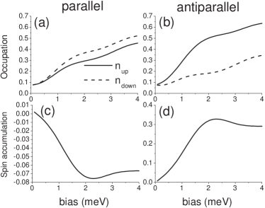
Figure 2: Spin-resolved occupations $n_{\uparrow}$ and $n_{\downarrow}$ and the spin accumulation, $m=n_{\uparrow}-n_{\downarrow}$, against bias voltage in both parallel and antiparallel FM lead alignments. In the P case $n_{\uparrow}<n_{\downarrow}$ while in the AP alignment $n_{\uparrow}>n_{\downarrow}$. These imbalances give rise to spin-dependent population suppressions in the bias range 1-3 meV. This translates into a tunable $m$ with the bias voltage. Parameters: $p_{L}=0.23$, $p_{R}=0.35$, $k_{B}T=200$ $\mu$eV, $\Gamma_{0}=10$ $\mu$eV, $\epsilon_{0}=0.5$ meV and $U=1$ meV.

Spin accumulation. In Fig. 2(c)-(d) we show the spin accumulation ($m=n_{\uparrow}-n_{\downarrow}$) as a function of the bias voltage. In the zero bias limit $m$ is essentially zero. When the bias increases the spin accumulation in the P case assume negative values. In contrast, in the AP alignment $m$ is enhanced. In particular, in the bias range corresponding to a singly-occupied dot (1-3 meV)singleocup the additional suppression [Fig. 2(c)] or the enhancement [Fig. 2(d)] of $m$ is due to the spin-dependent population suppression that takes place in the presence of Coulomb interaction and spin accumulation. More specifically, in the AP case due to Coulomb interaction $n_{\uparrow}$ tends to suppress more strongly $n_{\downarrow}$ than otherwise. This translates into an enhancement of $m$. In the P alignment the spin up occupation $n_{\uparrow}$ is more suppressed than $n_{\downarrow}$, thus $m$ becomes more negative [Fig. 2(c)]. We emphasize that this effect happens for both the P and AP alignments because we assume $p_{L}\neq p_{R}$. For equal leads we find $n_{\uparrow}=n_{\downarrow}$ in the P case so that $m$ remains zero in this configuration.

IV.2 Current and its polarization

Current. Figures 3(a)-(b) show the current in the P and AP cases for $U=1$ meV and $R=0$. Similarly to the occupations, some features of the spin-up and spin down currents can be understood in terms of the tunneling rates. For instance, their saturation values (second plateau) can be easily calculated from the standard expresssionstandardeq

$$I^{\sigma}_{\eta}=e\frac{\Gamma_{\sigma}^{L}\Gamma_{\sigma}^{R}}{\Gamma_{\sigma}^{L}+\Gamma_{\sigma}^{R}},$$ (36)

which gives $I^{\uparrow}_{\eta}>I^{\downarrow}_{\eta}$ and $I^{\uparrow}_{\eta}<I^{\downarrow}_{\eta}$ in the P and AP cases, respectively. For the first plateau Eq. (36) is not valid and these inequalities can change.at03

In the P case [Fig. 3(c)] $I_{\uparrow}$ is more strongly suppressed than $I_{\downarrow}$ due to the interplay of spin accumulation ($n_{\uparrow}<n_{\downarrow}$) and Coulomb interaction. This results in a supression of the current polarization [$\wp=(I_{\uparrow}-I_{\downarrow})/(I_{\uparrow}+I_{\downarrow})$] in the range 1-3 meV. On the other hand, in the AP case [Fig. 3(d)] $I^{\downarrow}_{\eta}$ is more suppressed than $I^{\uparrow}_{\eta}$ due to the inverted inequality $n_{\uparrow}>n_{\downarrow}$, thus resulting in an enhancement of $\wp$.

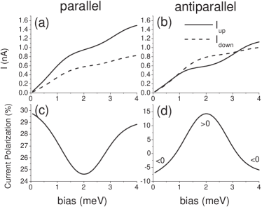
Figure 3: (a)-(b) Spin-resolved currents $I_{\uparrow}$ and $I_{\downarrow}$ and (c)-(d) current polarization for both parallel and antiparallel alignments. In the P case we find $I_{\uparrow}>I_{\downarrow}$. In contrast, for AP alignment $I_{\uparrow}<I_{\downarrow}$ in the bias window $1-3$ meV (singly occupied regime) and $I_{\uparrow}>I_{\downarrow}$ when the bias exceeds the charging energy above $3$ meV (doubly occupied regime). Panels (c)-(d) reveal a suppression and an enhancement of the current polarization in the singly occupied regime for the P and AP cases, respectively. Parameters: $p_{L}=0.23$, $p_{R}=0.35$, $k_{B}T=200$ $\mu$eV, $\Gamma_{0}=10$ $\mu$eV, $R=0$, $\epsilon_{0}=0.5$ meV and $U=1$ meV.

Spin-flip effects. In figure (4) we show the current polarization against bias voltage for distinct spin-flip parameter $R$. The polarization is calculated for the left and right leads, according to the formula $\wp^{\eta}=(I^{\uparrow}_{\eta}-I^{\downarrow}_{\eta})/(I^{\uparrow}_{\eta}+I^{\downarrow}_{\eta})$, where $\eta=L,R$. For $R=0$ (solid line) we have $\wp^{L}=\wp^{R}$ for all biases. This curve is the same as seen in Fig. 3(d). When $R\neq 0$ these two polarizations depart from each other. The $\wp^{L}$ increases with $R$ tending to reach the left lead polarization value $p_{L}=0.23$. In contrast, $\wp^{R}$ assume negative values tending to $-p_{R}$ as $R$ increases. This shows that even though we have a constant total current along the system ($I_{L}^{\uparrow}+I_{L}^{\downarrow}=I_{R}^{\uparrow}+I_{R}^{\downarrow}$), its polarization can change across the system when $R\neq 0$, i.e., when there is a transverse magnetic field applied on the dot which coherently rotates the spin.

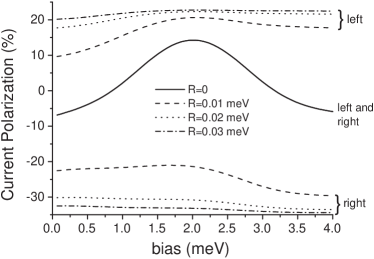
Figure 4: Current polarization against the bias voltage for differing spin-flip rates in the AP alignment and in both left and right leads. For $R=0$ the polarization is the same on both sides. When $R\neq 0$, though, the current polarization in the left side enhances, tending to the left magnetization degree $p_{L}$. In contrast, the current polarization in the right side assumes negative values, tending to $-p_{R}$. Parameters: $p_{L}=0.23$, $p_{R}=0.35$, $k_{B}T=200$ $\mu$eV, $\Gamma_{0}=10$ $\mu$eV, $\epsilon_{0}=0.5$ meV and U=1 meV.

Figure 5 shows $I_{\eta}^{\sigma}$ against $R$. For $R=0$, $I^{\uparrow}_{L}=I^{\uparrow}_{R}$ and $I_{L}^{\downarrow}=I_{R}^{\downarrow}$ as expected. For $R\neq 0$ these equalities disappear, with $I_{L}^{\uparrow}$ and $I_{R}^{\downarrow}$ increasing and $I_{L}^{\downarrow}$ and $I_{R}^{\uparrow}$ decreasing with $R$. This leads to an enhancement of $\wp^{L}$ and $|\wp_{R}|$ as seen in Fig. 4. Interestingly, there is a crossing point between $I_{L}^{\uparrow}$ and $I_{L}^{\downarrow}$ around $R\approx\Gamma_{0}/4$. So for this particular $R$ the total current becomes unpolarized in the emitter (left) lead and relatively high polarized in the collector (right) lead. This means that it is possible to change the current polarization from emitter to collector lead by precessing the electron spin in the quantum dot.

In the inset of Fig. 5 we show the total current against $R$. This curve resembles a typical Hanle resonance.hanle ; mb05 Similarly to Ref. [mb05, ], here we can say that in the AP configuration and positive bias (i.e., with left being the emitter) the dot tends to be more up populated due to the majority up population in the emitter and the majority down population in the collector lead. On average a transverse magnetic field tends to increase the spin down component in the dot along the down magnetization of the collector lead. As a result the electron can more easily tunnel into the right ferromagnet and the current increases.

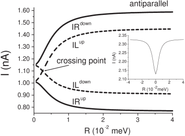
Figure 5: Spin-resolved currents versus $R$. For $R=0$ we have $I_{L}^{\uparrow}=I_{R}^{\uparrow}$ and $I_{L}^{\downarrow}=I_{R}^{\downarrow}$ with $I_{\eta}^{\uparrow}$ and $I_{\eta}^{\downarrow}$ being different from each other. For increasing $R$, $I_{L}^{\uparrow}$ and $I_{R}^{\downarrow}$ grow while $I_{L}^{\downarrow}$ and $I_{R}^{\uparrow}$ decreases. For a particular $R$ there is a crossing between $I_{L}^{\uparrow}$ and $I_{L}^{\downarrow}$, thus resulting simultaneously in a non-polarized left-current and a polarized right-current. Parameters: $p_{L}=0.23$, $p_{R}=0.35$, $k_{B}T=200$ $\mu$eV, $\Gamma_{0}=10$ $\mu$eV, $\epsilon_{0}=0.5$ meV, U=1 meV and bias=4 meV.

IV.3 Shot Noise

Figure 6 shows the Fano factor, $\gamma=S_{LL}/2eI_{L}$, against $R$ in the AP configurations. The P alignment gives approximately insensitive Fano factor with respect to $R$. In the AP configuration, the Fano factor can be suppressed with $R$, reaching values below 0.5. This suppression can be further intensified by increasing the lead polarization parameters $p_{L}$ and $p_{R}$. In particular, for fully spin-polarized leads ($p=1$) AP aligned, the Fano factor reaches values close to 0.3 when double occupancy is allowed (bias = 6 meV) and it attains 0.35 in the single occupancy regime (bias = 2 meV).fgb02 For fully polarized leads in the P configuration the Fano factor remains at 0.5 independently of $R$.

A simple physical picture for this additional suppression of $\gamma$ is as follows. Consider an up spin sitting on the dot. A second up spin trying to hop onto it is Pauli blocked, till the first electron tunnel to the collector lead or undergo a coherent spin-flip. If the spin-flip is fast enough (faster than the into/out tunneling processes) the first electron can return to its original state (via another spin-flip), instead of tunneling out of the dot. This blocks additionally the second up spin, consequently suppressing even further the noise.

We note that for any $R$ when we go from the single (bias = 2 meV) to the double (bias = 6 meV) occupation regimes a reduction of the Fano factor is observed in both P and AP alignments (cf. solid black to solid gray lines and dashed black to dashed gray lines). This general feature was already predicted in Ref. [mb06, ], where a diagrammatic formulation for the noise is derived. It is valid to mention that in the present study we have performed an S-matrix expansion (Appendix B) to the noise which could in principle be mapped into a Feynman diagrammatic formulation. Comparing our results with previous findings in the literature we observe a difference between them in the single-occupancy regime.singleocup Figure 7 shows a comparison for the shot noise obtained from Eq. (33) and from analytical results in Ref. [at03, ] (derived for $p_{L}=p_{R}=0$ and $R=0$). While the second plateau [II in Fig. (7)] coincides in both numerical and analytical cases, the first plateaus (I in the plot) do not coincide.comparison This disagreement is related to the Hartree-Fock factorization underlying our calculation.

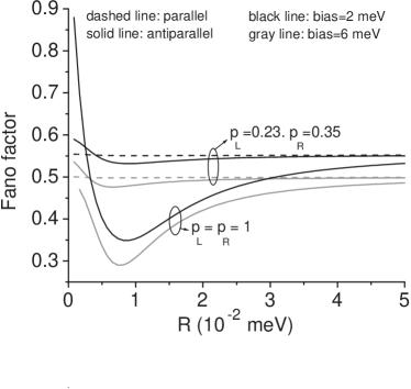
Figure 6: Fano factor against $R$ for two fixed bias voltages corresponding to single (bias = 2 meV) and double occupancy (bias = 6 meV) in both P and AP alignments. In the P case the Fano factor is approximatelly constante. In contrast, in the AP alignment the Fano factor can be suppressed due to spin-flip, reaching values below 0.5. In particular, for fully polarized leads ($p_{L}=p_{R}=1$) the Fano factor can be strongly suppressed, assuming values close to 0.3 when double occupancy is allowed. Parameters: $\epsilon_{0}=0.5$ meV, $U=1$ meV, $\Gamma_{0}=10$ $\mu$eV and $k_{B}T=200$ $\mu$eV.

It is yet valid to note that without Coulomb interaction ($U=0$) and for fully spin polarized leads antiparallel aligned, the Fano factor is given by

$$\gamma=1-\frac{1}{2}\frac{\beta^{2}(5+\beta^{2})}{(1+\beta^{2})^{2}},$$ (37)

where $\beta=R/\Gamma_{0}$. Eq. (37) is also found for a three tunneling barriers junction.hbs97 Hence, for fully spin-polarized AP leads and non-vanishing spin-flip, the FM-QD-FM setup resembles a three-barrier geometry.

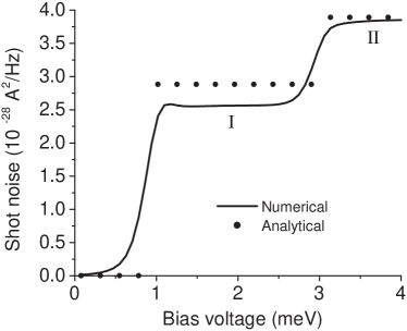
Figure 7: Comparison of the shot noise for the present approach (numerical) and the one derived in Ref. [at03, ] (analytical). While the second plateau (II) coincides in both approaches, the first plateau (I) differs. We attribute this contrast to the Hartree-Fock type approximation used in our calculation. Parameters: $p_{L}=p_{R}=0$, $k_{B}T=50$ $\mu$eV, $\Gamma_{0}=10$ $\mu$eV , $R=0$, $\epsilon_{0}=0.5$ meV and $U=1$ meV.

V CONCLUSION

Using the nonequilibrium Green-function technique we have studied the transport properties of a quantum dot coupled to two ferromagnetic leads. We consider both parallel (P) and antiparallel (AP) alignments of the lead polarizations. Coulomb interaction and coherent spin-flip are included in our model. We find that for distinct ferromagnetic leads the interplay between Coulomb interaction and spin accumulation translates into an enhancement and a suppression of the current polarization $\wp$ in AP and P cases, respectively, depending on the bias. We also observe that the spin-flip can change the current polarization when it flows from the emitter to the collector. It is even possible to have a polarized current in the collector while it is unpolarized in the emitter. We have derived an expression for the noise [Eq. (33)] which exactly accounts for spin-flip but only approximately for Coulomb interaction. Finally, we found a suppression of the Fano factor to values well below 1/2 due to spin-flip.

The authors acknowledge support for this work from the Brazilian agencies CNPq, CAPES, FAPESP and IBEM and the FiDiPro program of the Finnish Academy. The authors thank J. König and J. Martinek for helpful discussions.

Appendix A Dot Green Functions

Here we present in some detail the calculation of the dot Green functions $\mathbf{G}^{r}$, $\mathbf{G}^{a}$, $\mathbf{G}^{>}$ and $\mathbf{G}^{<}$, used in the current and noise expressions. The starting point is to derive an equation of motion for the contour-ordered Green function $G_{\sigma\sigma^{\prime}}(\tau,\tau^{\prime})=-i\langle T_{c}d_{\sigma}(\tau)d_{\sigma^{\prime}}^{\dagger}(\tau^{\prime})\rangle$, and then, via analytical continuation rules, to determine these Green functions. After a straightforward calculation via equation of motion we find

$$\mathbf{G}(\tau,\tau^{\prime}) = \mathbf{G}^{0}(\tau,\tau^{\prime})$$ (38)

$$+ \int\int d\tau_{1}d\tau_{2}\mathbf{G}^{0}(\tau,\tau_{1})\mathbf{\Sigma}(\tau_{1},\tau_{2})\mathbf{G}(\tau_{2},\tau^{\prime})$$

$$+ \int d\tau_{1}\mathbf{G}^{0}(\tau,\tau_{1})U\mathbf{G}^{(2)}(\tau_{1},\tau^{\prime}),$$

where the components of $\mathbf{G}^{(2)}$ and $\mathbf{\Sigma}$ are $G_{ij}^{(2)}(\tau,\tau^{\prime})=-i\langle T_{c}n_{\overline{i}}(\tau)d_{i}(\tau)d_{j}^{\dagger}(\tau^{\prime})\rangle$, and $\Sigma_{ij}(\tau,\tau^{\prime})=\sum_{k\eta\sigma}\frac{1}{2}(-1)^{(i+j)\delta_{\sigma\downarrow}}|t_{k\sigma}|^{2}g_{k\sigma\eta}(\tau,\tau^{\prime})$, respectively. $\mathbf{G}^{0}$ is the dot Green function without both the coupling to leads and the Coulomb interaction.

Following the equation of motion expansion we find for $\mathbf{G}^{(2)}(\tau_{1},\tau^{\prime})$,

$$\mathbf{G}^{(2)}(\tau_{1},\tau^{\prime}) = \mathbf{G}^{0(2)}(\tau_{1},\tau^{\prime})+\int\int d\tau_{2}d\tau_{3}\mathbf{G}^{0(2)}(\tau_{1},\tau_{2})$$ (39)

$$\times \mathbf{\Sigma}(\tau_{2},\tau_{3})\mathbf{G}(\tau_{3},\tau^{\prime}),$$

where $\mathbf{G}^{0(2)}(\tau_{1},\tau^{\prime})$ satisfies the identity

$$(i\frac{\partial}{\partial\tau}-\epsilon_{i}-U)G_{ij}^{0(2)}(\tau,\tau^{\prime}) = \delta_{ij}\delta(t-t^{\prime})\langle n_{\overline{i}}\rangle-$$ (40)

$$\delta_{\overline{i}j}\delta(t-t^{\prime})\langle d_{\overline{i}}^{\dagger}d_{i}\rangle.$$

In Eq. (39) we have used the following approximations,standard_approx

$$\langle Td_{\overline{i}}(t)d_{i}(t)c_{k\sigma\eta}^{\dagger}(t)d_{j}^{\dagger}(t^{\prime})\rangle = 0$$

$$\langle Td_{\overline{i}}^{\dagger}(t)d_{i}(t)c_{k\sigma\eta}(t)d_{j}^{\dagger}(t^{\prime})\rangle = \langle d_{\overline{i}}^{\dagger}d_{i}\rangle\langle Tc_{k\sigma\eta}(t)d_{j}^{\dagger}(t^{\prime})\rangle$$

$$\langle Td_{\overline{i}}^{\dagger}(t)d_{\overline{i}}(t)c_{k\sigma\eta}(t)d_{j}^{\dagger}(t^{\prime})\rangle = \langle d_{\overline{i}}^{\dagger}d_{\overline{i}}\rangle\langle Tc_{k\sigma\eta}(t)d_{j}^{\dagger}(t^{\prime})\rangle.$$

Observe that Eq.(39) closes the system of equations (38)-(39). Substituting (39) into (38) we find a Dyson equation for $\mathbf{G}$

$$\mathbf{G}(\tau,\tau^{\prime}) = \widetilde{\mathbf{G}}^{0}(\tau,\tau^{\prime})+\int\int d\tau_{1}d\tau_{2}\widetilde{\mathbf{G}}^{0}(\tau,\tau_{1})$$ (41)

$$\times \mathbf{\Sigma}(\tau_{1},\tau_{2})\mathbf{G}(\tau_{2},\tau^{\prime}),$$

where

$$\widetilde{\mathbf{G}}^{0}(\tau,\tau^{\prime})=\mathbf{G}^{0}(\tau,\tau^{\prime})+\int d\tau_{1}\mathbf{G}^{0}(\tau,\tau_{1})U\mathbf{G}^{0(2)}(\tau_{1},\tau^{\prime}).$$ (42)

Applying analytical continuation rules in Eqs. (41) and (42) we find

$$\mathbf{G}^{r}(t,t^{\prime}) = \widetilde{\mathbf{G}}^{0r}(t,t^{\prime})+\int\int dt_{1}dt_{2}\widetilde{\mathbf{G}}^{0r}(t,t_{1})$$ (43)

$$\times \mathbf{\Sigma}^{r}(t_{1},t_{2})\mathbf{G}^{r}(t_{2},t^{\prime}),$$

$$\widetilde{\mathbf{G}}^{0r}(t,t^{\prime})=\mathbf{G}^{0r}(t,t^{\prime})+\int dt_{1}\mathbf{G}^{0r}(t,t_{1})U\mathbf{G}^{0(2)}(t_{1},t^{\prime}),$$ (44)

and also the Keldysh equation

$$\mathbf{G}^{<}(t,t^{\prime})=\int\int dt_{1}dt_{2}\mathbf{G}^{r}(t,t_{1})\mathbf{\Sigma}^{<}(t_{1},t_{2})\mathbf{G}^{a}(t_{2},t^{\prime}).$$ (45)

Via Fourier transform of Eqs. (43) and (44) we obtain

$$\mathbf{G}^{r}(\epsilon)=[\widetilde{\mathbf{G}}^{0r^{-1}}(\epsilon)-\mathbf{\Sigma}^{r}(\epsilon)]^{-1},$$ (46)

$$\widetilde{\mathbf{G}}^{0r}(\epsilon)=\mathbf{G}^{0r}(\epsilon)+\mathbf{G}^{0r}(\epsilon)U\mathbf{G}^{0(2)}(\epsilon),$$ (47)

and of Eq. (45) we find

$$\mathbf{G}^{<}(\epsilon)=\mathbf{G}^{r}(\epsilon)\mathbf{\Sigma}^{<}(\epsilon)\mathbf{G}^{a}(\epsilon),$$ (48)

where

$$\mathbf{G}^{0r}(\epsilon)=\left(\begin{array}[]{cc}\frac{1}{\epsilon-\epsilon_{1}+i0^{+}}&0\\ 0&\frac{1}{\epsilon-\epsilon_{2}+i0^{+}}\end{array}\right)$$ (49)

and

$$\mathbf{G}^{0(2)r}(\epsilon)=\left(\begin{array}[]{cc}\frac{\langle n_{2}\rangle}{\epsilon-\epsilon_{1}-U+i0^{+}}&-\frac{\langle d_{2}^{\dagger}d_{1}\rangle}{\epsilon-\epsilon_{1}-U+i0^{+}}\\ -\frac{\langle d_{1}^{\dagger}d_{2}\rangle}{\epsilon-\epsilon_{2}-U+i0^{+}}&\frac{\langle n_{1}\rangle}{\epsilon-\epsilon_{2}-U+i0^{+}}\end{array}\right).$$ (50)

The retarded self energy is given by

$$\Sigma^{r}=-\frac{i}{2}\left(\begin{array}[]{cc}\Gamma_{\uparrow}+\Gamma_{\downarrow}&\Gamma_{\uparrow}-\Gamma_{\downarrow}\\ \Gamma_{\uparrow}-\Gamma_{\downarrow}&\Gamma_{\uparrow}+\Gamma_{\downarrow}\end{array}\right),$$ (51)

and the lesser self energy is defined as

$$\Sigma_{lm}^{<}=\sum_{\sigma}\frac{i}{2}(-1)^{(l+m)\delta_{\sigma\downarrow}}(n_{L}\Gamma_{\sigma}^{L}+n_{R}\Gamma_{\sigma}^{R}).$$ (52)

Appendix B S-matrix expansion for the noise

According to Eq. (24) the noise is given in terms of the four-operator Green functions $g^{(2)}_{i}(\tau,\tau^{\prime})$ [$i=1,2,3,4$]. To determine their equations of motion we develop an $S$-matrix expansion as we illustrate below for $g^{(2)}_{1}(\tau,\tau^{\prime})$. The first step is to transform the operators from the Heisenberg to the interaction picture,

$$g^{(2)}_{1}(\tau,\tau^{\prime}) = i^{2}\langle T_{c}S\widetilde{c}_{k\sigma\eta}^{\dagger}(\tau)\widetilde{d}_{i}(\tau)\widetilde{c}_{k^{\prime}\sigma^{\prime}\eta^{\prime}}^{\dagger}(\tau^{\prime})\widetilde{d}_{j}(\tau^{\prime})\rangle,$$

where the tilde denotes the operators in the interaction picture, i.e.,

$$d_{i}(t)=v^{\dagger}(t,t_{0})\widetilde{d}_{i}(t)v(t,t_{0}),$$ (53)

with

$$v(t,t_{0})=Te^{-i\int_{t_{0}}^{t}dt^{\prime}\widetilde{H}_{T}(t^{\prime})},$$ (54)

and a similar definition for the $c$ operator. The operator $T$ is the time-ordering operator. The $S$-matrix in $g^{(2)}_{1}(\tau,\tau^{\prime})$ is defined as

$$S=T_{c}e^{-i\int_{c}d\tau_{1}\widetilde{H}_{T}(\tau_{1})}.$$ (55)

Expanding $S$ we find

$$g^{(2)}_{1}(\tau,\tau^{\prime})=i^{2}\sum_{n=0}^{\infty}\frac{(-i)^{n}}{n!}$$

$$\phantom{xx}\times\langle T_{c}\widetilde{c}_{k\sigma\eta}^{\dagger}(\tau)\widetilde{d}_{i}(\tau)\widetilde{c}_{k^{\prime}\sigma^{\prime}\eta^{\prime}}^{\dagger}(\tau^{\prime})\widetilde{d}_{j}(\tau^{\prime})$$

$$\times[\int d\tau_{1}\sum_{k_{1}\sigma_{1}\eta_{1}i_{1}}\frac{(-1)^{i_{1}\delta_{\sigma_{1}\downarrow}}}{\sqrt{2}}(t_{k_{1}\sigma_{1}}\widetilde{c}_{k_{1}\sigma_{1}\eta_{1}}^{\dagger}(\tau_{1})\widetilde{d}_{i_{1}}(\tau_{1})$$

$$\phantom{xxxxxxx}+t_{k_{1}\sigma_{1}}^{*}\widetilde{d}_{i_{1}}^{\dagger}(\tau_{1})\widetilde{c}_{k_{1}\sigma_{1}\eta_{1}}(\tau_{1})]^{n}\rangle,$$ (56)

where the lowest-order nonzero term in the expansion is that of $n=2$. Since we assume noninteracting leads, we can factorize the angle bracket in Eq. (56) into a product of the lead and dot parts. We then apply Wick’s theorem to the lead part. This results in

$$g^{(2)}_{1}(\tau,\tau^{\prime}) = t_{k\sigma}^{*}t_{k^{\prime}\sigma^{\prime}}^{*}\int\int d\tau_{1}d\tau_{2}\sum_{k_{1}\sigma_{1}\eta_{1}}\sum_{k_{2}\sigma_{2}\eta_{2}}$$ (57)

$$\sum_{i_{1}i_{2}=1,2}\frac{1}{2}(-1)^{i_{1}\delta_{\sigma_{1}\downarrow}}(-1)^{i_{2}\delta_{\sigma_{2}\downarrow}}$$

$$(-i)\langle T_{c}\widetilde{c}_{k_{1}\sigma_{1}\eta_{1}}(\tau_{1})\widetilde{c}_{k\sigma\eta}^{\dagger}(\tau)\rangle$$

$$(-i)\langle T_{c}\widetilde{c}_{k_{2}\sigma_{2}\eta_{2}}(\tau_{2})\widetilde{c}_{k^{\prime}\sigma^{\prime}\eta^{\prime}}^{\dagger}(t^{\prime})\rangle$$

$$\langle T_{c}S\widetilde{d}_{i}(\tau)\widetilde{d}_{j}(\tau^{\prime})\widetilde{d}_{i_{1}}^{\dagger}(\tau_{1})\widetilde{d}_{i_{2}}^{\dagger}(\tau_{2})\rangle.$$

In Eq. (57) we have contracted $\widetilde{c}_{k_{1}\sigma_{1}\eta_{1}}$ with $\widetilde{c}_{k\sigma\eta}^{\dagger}$, and $\widetilde{c}_{k_{2}\sigma_{2}\eta_{2}}$ with $\widetilde{c}^{\dagger}_{k^{\prime}\sigma^{\prime}\eta^{\prime}}$. This is one choice among $n(n-1)$ possible contractions. Since all of them yields the same result, we simply multiply the chosen pairing by $n(n-1)$. This factor cancels part of the factorial $n!$ in Eq.(56), thus resulting in the $S$-matrix in the last angle bracket of Eq. (57).

The first and second averages in (57) give $\delta_{k\sigma\eta,k_{1}\sigma_{1}\eta_{1}}$ and $\delta_{k^{\prime}\sigma^{\prime}\eta^{\prime},k_{2},\sigma_{2},\eta_{2}}$, respectively, so the sums over $(k_{1},\sigma_{1},\eta_{1})$ and $(k_{2},\sigma_{2},\eta_{2})$ disappear. Defining $g_{k\sigma\eta}(\tau_{1},\tau)=-i\langle T_{c}\widetilde{c}_{k\sigma\eta}(\tau_{1})c_{k\sigma\eta}^{\dagger}(\tau)\rangle$ and $g_{k^{\prime}\sigma^{\prime}\eta^{\prime}}(\tau^{\prime},\tau_{2})=-i\langle T_{c}\widetilde{c}_{k^{\prime}\sigma^{\prime}\eta^{\prime}}(\tau^{\prime})\widetilde{c}_{k^{\prime}\sigma^{\prime}\eta^{\prime}}^{\dagger}(\tau_{2})\rangle$, we can rewrite (57) as

$$g^{(2)}_{1}(\tau,\tau^{\prime})=t_{k\sigma}^{*}t_{k^{\prime}\sigma^{\prime}}^{*}\int\int d\tau_{1}d\tau_{2}$$

$$\times \sum_{i_{1},i_{2}=1,2}\frac{1}{2}(-1)^{i_{1}\delta_{\sigma_{1}\downarrow}}(-1)^{i_{2}\delta_{\sigma_{2}\downarrow}}$$

$$\times g_{k\sigma\eta}(\tau_{1},\tau)g_{k^{\prime}\sigma^{\prime}\eta^{\prime}}(\tau_{2},\tau^{\prime})\langle T_{c}d_{i}(\tau)d_{j}(\tau^{\prime})d_{i_{1}}^{\dagger}(\tau_{1})d_{i_{2}}^{\dagger}(\tau_{2})\rangle.$$

For the $U=0$ case the calculation is straightforward. By applying Wick’s theorem in the four operators Green function, we find

$$g^{(2)}_{1}(\tau,\tau^{\prime})=t_{k\sigma}^{*}t_{k^{\prime}\sigma^{\prime}}^{*}\int\int d\tau_{1}d\tau_{2}$$

$$\phantom{x}\times\sum_{i_{1}i_{2}}\frac{1}{2}(-1)^{i_{1}\delta_{\sigma\downarrow}}(-1)^{i_{2}\delta_{\sigma^{\prime}\downarrow}}g_{k\sigma\eta}(\tau_{1},\tau)g_{k^{\prime}\sigma^{\prime}\eta^{\prime}}(\tau_{2},\tau^{\prime})$$

$$\phantom{x}\times\{G_{ii_{1}}(\tau,\tau_{1})G_{ji_{2}}(\tau^{\prime},\tau_{2})-G_{ii_{2}}(\tau,\tau_{2})G_{ji_{1}}(\tau^{\prime},\tau_{1})\}$$

where $G_{ii_{1}}(\tau,\tau_{1})=-i\langle T_{c}d_{i}(\tau)d_{i_{1}}^{\dagger}(\tau_{1})\rangle$, plus analogous definitions for the other Green functions. A similar calculation yields Eq. (III.4) for $g^{(2)}_{2}(\tau,\tau^{\prime})$. In the presence of the Coulomb interaction ($U\neq 0$) Eq. (B) is no longer exact and the full diagrammatic expansion should be considered in order to find an accurate noise expression. However, this is a formidable task since it involves not only the usual many body expansion but also the analytical continuation of two and more particles Green functions. So as a first approximation we use Eq. (B) even in the presence of the Coulomb interaction.

Appendix C “Linked-Cluster Theorem” for the noise expansion

Equations (III.4)-(28) are composed of what we call connected and disconnected terms. Here we show that the disconnected parts cancel identically the term $2I_{\eta}^{2}$ in Eq. (24). Writing explicitly the disconnected term of Eq.(III.4), we have

$$g_{1\rm{disc}}^{(2)}(\tau,\tau^{\prime})=t_{k\sigma}^{\ast}t_{k^{\prime}\sigma^{\prime}}^{\ast}\sum_{i_{1}i_{2}}\frac{1}{2}(-1)^{i_{1}\delta_{\sigma\downarrow}}(-1)^{i_{2}\delta_{\sigma^{\prime}\downarrow}}$$

$$\phantom{xxxxxx}\times\int d\tau_{1}G_{ii_{1}}(\tau,\tau_{1})g_{k\sigma\eta}(\tau_{1},\tau^{+})$$

$$\phantom{xxxxxx}\times\int d\tau_{2}G_{ji_{2}}(\tau^{\prime},\tau_{2})g_{k^{\prime}\sigma^{\prime}\eta^{\prime}}(\tau_{2},\tau^{\prime+}),$$ (59)

where the $+$ sign on one of the $\tau$ and $\tau^{\prime}$ is just reminder that the sequence of operators $c_{k\sigma\eta}^{\dagger}(\tau)d_{i}(\tau)$ and $c_{k^{\prime}\sigma^{\prime}\eta^{\prime}}^{\dagger}(\tau^{\prime})d_{j}(\tau^{\prime})$ in the main definition of $g_{1}^{(2)}(\tau,\tau^{\prime})$ (beginning of Sec. III-D) should be preserved during the following calculation. Applying the analytic continuation rules we obtain

$$g_{1\rm{disc}}^{(2)>}(t,t^{\prime}) = t_{k\sigma}^{\ast}t_{k^{\prime}\sigma^{\prime}}^{\ast}$$ (60)

$$F_{i\sigma,k\eta\sigma}(t,t)F_{j\sigma^{\prime},k^{\prime}\eta^{\prime}\sigma^{\prime}}(t^{\prime},t^{\prime}),$$

with

$$F_{i\sigma,k\eta\sigma}(t,t)=\sum_{i_{1}}\frac{1}{\sqrt{2}}(-1)^{i_{1}\delta_{\sigma\downarrow}}\int dt_{1}\times$$

$$\phantom{x}[G_{ii_{1}}^{r}(t,t_{1})g_{k\sigma\eta}^{<}(t_{1},t)+G_{ii_{1}}^{<}(t,t_{1})g_{k\sigma\eta}^{a}(t_{1},t)],$$ (61)

and a similar definition for $F_{j\sigma^{\prime},k^{\prime}\eta^{\prime}\sigma^{\prime}}(t^{\prime},t^{\prime})$. Similarly, from Eq. (III.4), we have

$$g^{(2)}_{2\rm{disc}}(\tau,\tau^{\prime})=t_{k\sigma}^{*}t_{k^{\prime}\sigma^{\prime}}\sum_{i_{1},i_{2}=1,2}\frac{1}{2}(-1)^{i_{1}\delta_{\sigma\downarrow}}(-1)^{i_{2}\delta_{\sigma^{\prime}\downarrow}}$$

$$\phantom{xxx}\times\int d\tau_{1}G_{ii_{1}}(\tau,\tau_{1})g_{k\sigma\eta}(\tau_{1},\tau^{+})$$

$$\phantom{xxx}\times\int d\tau_{2}g_{k^{\prime}\sigma^{\prime}\eta^{\prime}}(\tau^{\prime},\tau_{2})G_{i_{2}j}(\tau_{2},\tau^{\prime+}).$$ (62)

which, after analytic continuation, can be expressed as

$$g_{2\rm{disc}}^{(2)>}(t,t^{\prime}) = -t_{k\sigma}^{\ast}t_{k^{\prime}\sigma^{\prime}}$$ (63)

$$F_{i\sigma,k\eta\sigma}(t,t)F_{j\sigma^{\prime},k^{\prime}\eta^{\prime}\sigma^{\prime}}^{\ast}(t^{\prime},t^{\prime}).$$

sing the identities Eqs. (27)-(28) we obtain

$$g_{3\rm{disc}}^{(2)>}(t,t^{\prime}) = -t_{k\sigma}t_{k^{\prime}\sigma^{\prime}}^{\ast}$$ (64)

$$F_{i\sigma,k\eta\sigma}^{\ast}(t,t)F_{j\sigma^{\prime},k^{\prime}\eta^{\prime}\sigma^{\prime}}(t^{\prime},t^{\prime}),$$

and

$$g_{4\rm{disc}}^{(2)>}(t,t^{\prime}) = t_{k\sigma}t_{k^{\prime}\sigma^{\prime}}$$ (65)

$$F_{i\sigma,k\eta\sigma}^{\ast}(t,t)F_{j\sigma^{\prime},k^{\prime}\eta^{\prime}\sigma^{\prime}}^{\ast}(t^{\prime},t^{\prime}).$$

From Eqs. (22) and (24) we note that

$$\langle\{\widehat{I}_{\eta}(t),\widehat{I}_{\eta^{\prime}}(t^{\prime})\}\rangle_{\rm{disc}} = e^{2}\sum_{kk^{\prime}\sigma\sigma^{\prime}ij}\frac{1}{2}(-1)^{i\delta_{\sigma\downarrow}}(-1)^{j\delta_{\sigma^{\prime}\downarrow}}$$ (66)

$$\{t_{k\sigma}t_{k^{\prime}\sigma^{\prime}}g_{1\rm{disc}}^{(2)>}(t,t^{\prime})$$

$$-t_{k\sigma}t_{k^{\prime}\sigma^{\prime}}^{\ast}g_{2\rm{disc}}^{(2)>}(t,t^{\prime})$$

$$-t_{k\sigma}^{\ast}t_{k^{\prime}\sigma^{\prime}}g_{3\rm{disc}}^{(2)>}(t,t^{\prime})$$

$$+t_{k\sigma}^{\ast}t_{k^{\prime}\sigma^{\prime}}^{\ast}g_{4\rm{disc}}^{(2)>}(t,t^{\prime})\}$$

$$+h.c.$$

Using Eqs. (C), (C), (64) and (65) in Eq. (66) we find

$$\langle\{\widehat{I}_{\eta}(t),\widehat{I}_{\eta^{\prime}}(t^{\prime})\}\rangle_{\rm{disc}}=2e^{2}\sum_{kk^{\prime}\sigma\sigma^{\prime}ij}|t_{k\sigma}|^{2}|t_{k^{\prime}\sigma^{\prime}}|^{2}$$

$$\frac{1}{2}(-1)^{i\delta_{\sigma\downarrow}}(-1)^{j\delta_{\sigma^{\prime}\downarrow}}[F_{i\sigma,k\eta\sigma}(t,t)+F_{i\sigma,k\eta\sigma}^{\ast}(t,t)]$$

$$\phantom{xxx}\times[F_{j\sigma^{\prime},k^{\prime}\eta^{\prime}\sigma^{\prime}}(t^{\prime},t^{\prime})+F_{j\sigma^{\prime},k^{\prime}\eta^{\prime}\sigma^{\prime}}^{\ast}(t^{\prime},t^{\prime})].$$ (67)

On the other hand we can write the current as

$$\langle\widehat{I}_{\eta}(t)\rangle = 2e\mathrm{Re}\sum_{k\sigma i}|t_{k\sigma}|^{2}\frac{(-1)^{i\delta_{\sigma\downarrow}}}{\sqrt{2}}F_{i\sigma,k\eta\sigma}(t,t).$$ (68)

$$= e\sum_{k\sigma i}|t_{k\sigma}|^{2}\frac{(-1)^{i\delta_{\sigma\downarrow}}}{\sqrt{2}}$$

$$\phantom{xxx}\times[F_{i\sigma,k\eta\sigma}(t,t)+F_{i\sigma,k\eta\sigma}^{\ast}(t,t)]$$

Squaring Eq. (68) and multiplying it by two, we find

$$2\langle\widehat{I}_{\eta}(t)\rangle\langle\widehat{I}_{\eta^{\prime}}(t^{\prime})\rangle=2e^{2}\sum_{kk^{\prime}\sigma\sigma^{\prime}ij}|t_{k\sigma}|^{2}|t_{k^{\prime}\sigma^{\prime}}|^{2}$$

$$\times\frac{1}{2}(-1)^{i\delta_{\sigma\downarrow}}(-1)^{j\delta_{\sigma^{\prime}\downarrow}}[F_{i\sigma,k\eta\sigma}(t,t)+F_{i\sigma,k\eta\sigma}^{\ast}(t,t)]$$

$$\phantom{xxxx}\times[F_{j\sigma^{\prime},k^{\prime}\eta^{\prime}\sigma^{\prime}}(t^{\prime},t^{\prime})+F_{j\sigma^{\prime},k^{\prime}\eta^{\prime}\sigma^{\prime}}^{\ast}(t^{\prime},t^{\prime})].$$ (69)

Hence, Eq. (C) cancels identically with (C), i.e.,

$$\langle\{\widehat{I}_{\eta}(t),\widehat{I}_{\eta^{\prime}}(t^{\prime})\}\rangle_{\rm{disc}}-2\langle\widehat{I}_{\eta}(t)\rangle\langle\widehat{I}_{\eta^{\prime}}(t^{\prime})\rangle=0.$$ (70)

Appendix D Recovering the Standard Formula for the Noise

To prove Eq. (III.5) we note that the Green functions appearing in Eq. (33) can be written as follow,

$$\mathbf{\Gamma}^{L}\mathbf{G}^{<}=i\mathbf{\Gamma}^{L}\mathbf{G}^{r}(n_{L}\mathbf{\Gamma}^{L}+n_{R}\mathbf{\Gamma}^{R})\mathbf{G}^{a},$$ (71)

$$\mathbf{\Gamma}^{L}\mathbf{G}^{>}=-i\mathbf{\Gamma}^{L}\mathbf{G}^{r}[(1-n_{L})\mathbf{\Gamma}^{L}+(1-n_{R})\mathbf{\Gamma}^{R}]\mathbf{G}^{a},$$ (72)

$$\mathbf{\Gamma}^{L}(\mathbf{G}^{r}-\mathbf{G}^{a})=-i\mathbf{\Gamma}^{L}\mathbf{G}^{r}(\mathbf{\Gamma}^{L}+\mathbf{\Gamma}^{R})\mathbf{G}^{a},$$ (73)

$$\mathrm{Tr}[\mathbf{\Gamma}^{L}\mathbf{G}^{a}\mathbf{\Gamma}^{L}\mathbf{G}^{a} + \mathbf{\Gamma}^{L}\mathbf{G}^{r}\mathbf{\Gamma}^{L}\mathbf{G}^{r}]=\mathrm{Tr}[2\mathbf{\Gamma}^{L}\mathbf{G}^{r}\mathbf{\Gamma}^{L}\mathbf{G}^{a}+\phantom{x}$$ (74)

$$\phantom{xx}\mathbf{\Gamma}^{L}(\mathbf{G}^{r}-\mathbf{G}^{a})\mathbf{\Gamma}^{L}(\mathbf{G}^{r}-\mathbf{G}^{a})].$$

Now, defining the generalized transmission coefficients

$$\mathbf{T}_{LL} = \mathbf{\Gamma}^{L}\mathbf{G}^{r}\mathbf{\Gamma}^{L}\mathbf{G}^{a}$$ (75)

$$\mathbf{T}_{LR} = \mathbf{\Gamma}^{L}\mathbf{G}^{r}\mathbf{\Gamma}^{R}\mathbf{G}^{a},$$ (76)

we can write the above set of equations [Eqs. (71)-(74)] in terms of $\mathbf{T}_{LL}$ and $\mathbf{T}_{LR}$,

$$\mathbf{\Gamma}^{L}\mathbf{G}^{<}=in_{L}\mathbf{T}_{LL}+in_{R}\mathbf{T}_{LR},$$ (77)

$$\mathbf{\Gamma}^{L}\mathbf{G}^{>}=-i(1-n_{L})\mathbf{T}_{LL}-i(1-n_{R})\mathbf{T}_{LR},$$ (78)

$$\mathbf{\Gamma}^{L}(\mathbf{G}^{r}-\mathbf{G}^{r})=-i\mathbf{T}_{LL}-i\mathbf{T}_{LR},$$ (79)

$$\mathrm{Tr}[\mathbf{\Gamma}^{L}\mathbf{G}^{a}\mathbf{\Gamma}^{L}\mathbf{G}^{a} + \mathbf{\Gamma}^{L}\mathbf{G}^{r}\mathbf{\Gamma}^{L}\mathbf{G}^{r}]=\mathrm{Tr}[2\mathbf{T}_{LL}-\phantom{xxxx}$$ (80)

$$(\mathbf{T}_{LL}+\mathbf{T}_{LR})(\mathbf{T}_{LL}+\mathbf{T}_{LR})].$$

Using Eqs. (77)-(80) in Eq. (33) we obtain

$$S_{LL}(\omega=0)=\frac{e^{2}}{\pi}\int d\epsilon\mathrm{Tr}\{$$

$$n_{L}(1-n_{L})\mathbf{T}_{LL}+n_{L}(1-n_{R})\mathbf{T}_{LR}$$

$$+(1-n_{L})n_{L}\mathbf{T}_{LL}+(1-n_{L})n_{R}\mathbf{T}_{LR}$$

$$+(n_{L}\mathbf{T}_{LL}+n_{R}\mathbf{T}_{LR})[(1-n_{L})\mathbf{T}_{LL}+(1-n_{R})\mathbf{T}_{LR}]$$

$$-n_{L}(\mathbf{T}_{LL}+\mathbf{T}_{LR})[(1-n_{L})\mathbf{T}_{LL}+(1-n_{R})\mathbf{T}_{LR}]$$

$$-(1-n_{L})(\mathbf{T}_{LL}+\mathbf{T}_{LR})[n_{L}\mathbf{T}_{LL}+n_{R}\mathbf{T}_{LR}]$$

$$-n_{L}(1-n_{L})[2\mathbf{T}_{LL}-(\mathbf{T}_{LL}+\mathbf{T}_{LR})(\mathbf{T}_{LL}+\mathbf{T}_{LR})]\}.$$

The terms with $\mathbf{T}_{LL}$ cancel out identically, and the above expression can be written as

$$S_{LL}(\omega=0)=\frac{e^{2}}{\pi}\int d\epsilon$$

$$\phantom{xxxx}\times\mathrm{Tr}\{[n_{L}(1-n_{L})+n_{R}(1-n_{R})]\mathbf{T}_{LR}(\epsilon)$$

$$\phantom{xxxxxx}+(n_{L}-n_{R})^{2}\mathbf{T}_{LR}(\epsilon)[1-\mathbf{T}_{LR}(\epsilon)]\}.$$ (81)

Denoting $\mathbf{T}_{LR}$ simply as $\mathbf{T}$ we arrive at Eq. (III.5).

References

- (1) S. Datta and B. Das, Appl. Phys. Lett. 56 (7), 665 (1990).
- (2) S. Cortez, O. Krebs, S. Laurent, M. Senes, X. Marie, P. Voisin, R. Ferreira, G. Bastard, J.-M. Gérard, and T. Amand, Phys. Rev. Lett. 89, 207401 (2002).
- (3) M. Kroutvar, Y. Ducommun, D. Heiss, M. Bichler, D. Schuh, G. Abstreiter, and J. J. Finley, Nature 432, 81 (2004).
- (4) D. D. Awschalom, D. Loss, and N. Samarth, Semiconductor Spintronics and Quantum Computation, Springer-Verlag, Berlin, (2002).
- (5) J. M. Elzerman, R. Hanson, L. H. W. van Beveren, B. Witkamp, L. M. K. Vandersypen, and L. P. Kouwenhoven, Nature 430, 431 (2004).
- (6) A. C. Johnson, J. R. Petta, J. M. Taylor, A. Yacoby, M. D. Lukin, C. M. Marcus, M. P. Hanson, and A. C. Gossard, Nature 435, 925 (2005).
- (7) F. H. L. Koppens, C. Buizert, K. J. Tielrooij, I. T. Vink, K. C. Nowack, T. Meunier, L. P. Kouwenhoven, and L. M. K. Vandersypen, Nature 442, 766 (2006).
- (8) M. A. Nielsen and I. L. Chuang, Quantum Computation and Quantum Information, Cambridge Univ. Press, Cambridge (2000).
- (9) M. Julliere, Phys. Lett. A 54, 225 (1975).
- (10) J. S. Moodera, L. R. Kinder, T. M. Wong and R. Meservey, Phys. Rev. Lett. 74, 3273 (1995).
- (11) M. N. Baibich, J. M. Broto, A. Fert, F. N. Van Dau, F. Petroff, P. Eitenne, G. Creuzet, A. Friederich, and J. Chazelas, Phys. Rev. Lett. 61, 2472 (1988).
- (12) K. Hamaya, S. Masubuchi, M. Kawamura, T. Machida, M. Jung, K. Shibata, K. Hirakawa, T. Taniyama, S. Ishida, and Y. Arakawa, Appl. Phys. Lett. 90, 053108 (2007).
- (13) K. Hamaya, M. Kitabatake, K. Shibata, M. Jung, M. Kawamura, K. Hirakawa, T. Machida, T. Taniyama, S. Ishida, and Y. Arakawa, Appl. Phys. Lett. 91, 022107 (2007).
- (14) A. N. Pasupathy, R. C. Bialczak, J. Martinek, J. E. Grose, L. A. K. Donev, P. L. McEuen, and D. C. Ralph, Science 306, 86 (2004).
- (15) S. Sahoo, T. Kontos, J. Furer, C. Hoffmann, M. Gräber, A. Cottet, and C. Schönenberger, Nat. Phys. 1, 99 (2005).
- (16) C. A. Merchant and N. Marković, arXiv:cond-mat/0710.2297.
- (17) I. Weymann and J. Barnaś, Phys. Rev. B 73, 33409 (2006).
- (18) I. Weymann, J. König, J. Martinek, J. Barnaś, and G. Schön, Phys. Rev. B 72,115334 (2005).
- (19) F. M. Souza, J. C. Egues, and A. P. Jauho, Phys. Rev. B 75, 165303 (2007).
- (20) This effect has been experimentally observed in Ref. [cam07, ].
- (21) F. Elsten and C. Timm, Phys. Rev. B 73, 235305 (2006).
- (22) A. Cottet, W. Belzig, and C. Bruder, Phys. Rev. Lett. 92, 206801 (2004).
- (23) A. Cottet and W. Belzig, Europhys. Lett. 66, 405 (2004).
- (24) M. P.-Ladrière, M. Ciorga, J. Lapointe, P. Zawadzki, M. Korkusiński, P. Hawrylak, and A. S. Sachrajda, Phys. Rev. Lett. 91, 026803 (2003).
- (25) F. M. Souza, Phys. Rev. B 76, 205315 (2007).
- (26) E. Perfetto, G. Stefanucci, and M. Cini, arXiv:cond-mat/0806.4480.
- (27) B. R. Bulka, J. Martinek, G. Michalek, and J. Barnaś, Phys. Rev. B 60, 12246 (1999).
- (28) Y. Tserkovnyak and A. Brataas, Phys. Rev. B 64, 214402 (2001).
- (29) E. G. Mishchenko, Phys. Rev. B 68, 100409(R) (2003).
- (30) M. Zareyan and W. Belzig, Phys. Rev. B 71, 184403 (2005).
- (31) R. Lopez and D. Sanchez, Phys. Rev. Lett. 90, 116602 (2003).
- (32) F. M. Souza, J. C. Egues, and A. P. Jauho, Proceedings of the 26th International Conference on the Physics of Semiconductors (ICPS 26), Edinburgh 2002, edited by J. H. Davies and A. R. Long. See arXiv:cond-mat/0209263.
- (33) D. Urban, M. Braun, and J. König, Phys. Rev. B 76, 125306 (2007).
- (34) A similar term has been used by a variety of authors describing spin-flip process in quantum dots, see for instance, P. Zhang, Q.-K. Xue, e X. C. Xie, Phys. Rev. Lett. 91, 196602 (2003), and Refs. [ep08, ], [rl03, ] and [wr01, ].
- (35) H. Engel and D. Loss, Phys. Rev. Lett. 86, 4648 (2001).
- (36) R. J. Epstein, D. T. Fuchs, W. V. Schoenfeld, P. M. Petroff, and D. D. Awschalom, Appl. Phys. Lett. 78, 733 (2001); L. Y. Zhang, C. Y. Wang, Y. G. Wei, X. Y. Liu, and D. Davidović, Phys. Rev. B 72, 155445 (2005).
- (37) M. Braun, J. König, and J. Martinek, Europhys. Lett. 72, 294 (2005).
- (38) Y. Meir and N. S. Wingreen, Phys. Rev. Lett. 68, 2512 (1992).
- (39) A. P. Jauho, N. S. Wingreen and Y. Meir, Phys. Rev. B 50, 5528 (1994).
- (40) L. V. Keldysh, Soviet. Physics JETP 20, 1018 (1965).
- (41) For a text-book treatment, see, e.g., H. Haug and A. P. Jauho, Quantum Kinetics in Transport and Optics of Semiconductors, Springer Solid-State Sciences 123 (1996).
- (42) M. Braun, J. König, and J. Martinek, Superlattices and Microstructures 37, 333 (2005).
- (43) For a review see Ya. M. Blanter and M. Büttiker, Phys. Rep. 336, 1 (2000).
- (44) A formally equivalent version of Eq. (33) has been published in the context of quantum dots with a phonon mode and Kondo physics, see J. X. Zhu and A. V. Balatsky, Phys. Rev. B 67, 165326 (2003) and B. Dong and X. L. Lei, J. Phys.: Condens. Matter 14, 4963 (2002), respectively.
- (45) G. B. Lesovik, Pisma v ZhETF 49, 513 (1989) [JETP Lett. 49, 592 (1989)]; V. A. Khlus, Zh. Ekps. Teor. Fiz. 93, 2179 (1987) [Sov. Phys. JETP 66, 1243 (1987)].
- (46) M. Büttiker, Phys. Rev. Lett. 65, 2901 (1990).
- (47) A diagrammatic formulation for the shot noise in a quantum dot coupled to ferromagnetic leads can be seen in [mb06, ].
- (48) F. M. Souza, J. C. Egues, and A. P. Jauho, Braz. J. Phys. 34, 565 (2004).
- (49) W. Rudziński and J. Barnaś, Phys. Rev. B 64, 085318 (2001).
- (50) Typical values of and can be found, for example, in D. G.-Gordon, H. Shtrikman, D. Mahalu, D. A.-Magder, U. Meirav, M. A. Kastner, Nature 391, 156 (1998). F. Simmel, R. H. Blick, J. P. Kotthaus, W. Wegscheider, and M. Bichler, Phys. Rev. Lett. 83, 804 (1999); A. Kogan et al., Phys. Rev. Lett. 93, 166602 (2004).
- (51) These parameters correspond to the polarization of Ni and Co, respectively. See R. Meservey and P. M. Tedrow, Phys. Rep. 238, 173 (1994).
- (52) In terms of the conduction channels single occupancy means and .
- (53) See, for instance, Eq. (76) of Ref. [ymb00, ].
- (54) For nonmagnetic leads, closed expressions for the current and the shot noise in all the plateaus can be found in A. Thielmann, M. H. Hettler, J. König, and G. Schön, Phys. Rev. B 68, 115105 (2003).
- (55) A suppression of the shot noise due to spin-flip can also be seen in F. G. Brito and J. C. Egues, Braz. J. Phys. 32, 324 (2002) and in I. Djuric, B. Dong, H. L. Cui, IEEE Transactions on Nanotechnology 4, 71, (2005).
- (56) M. Braun, J. König, and J. Martinek, Phys. Rev. B 74, 075328 (2006).
- (57) Comparing the current plateaus obtained from Eq. (16) and the ones derived in Ref. [at03, ] we find a complete agreement between the results.
- (58) H. B. Sun and G. J. Milburn, Superlattices and Microstructures 23, 883 (1997).
- (59) Y. P. Li, A. Zaslavsky, D. C. Tsui, M. Santos, and M. Shayegan, Phys. Rev. B 41, 8388 (1990).
- (60) J. H. Davies, J. C. Egues, and J. Wilkins, Phys. Rev. B 52, 11259 (1995). In this work, shot noise in a Fabry-Perot type model with dephasing leads was analyzed and it was found an enhancement of the Fano factor.
- (61) See Chapter 12 of Ref. [hh96, ] for a discussion about this kind of approximation.